
Temporal Prediction of Landslide-Generated Waves Using a Theoretical–Statistical Combined Method

Abstract
1. Introduction
2. Theoretical Basis
2.1. Physical Model
2.2. Empirical Equations
2.3. Slide Parameters Selected for the Temporal Prediction
3. Model Development
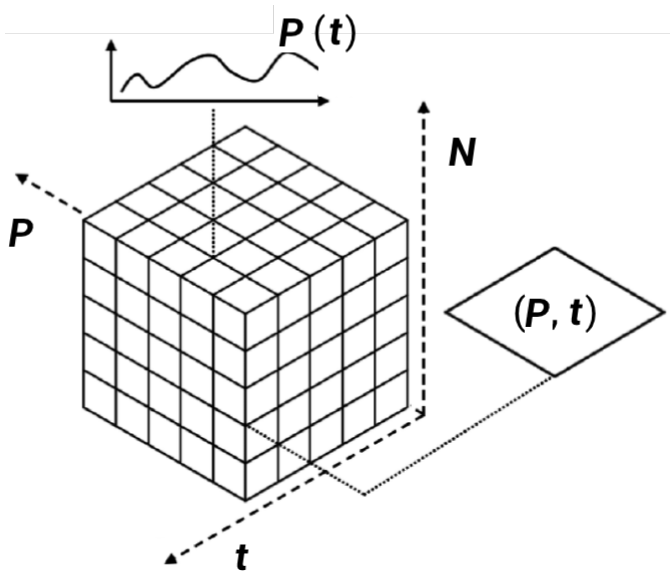
3.1. Panel Data Analysis
3.2. Theoretical Solutions of the Temporal Slide Thickness and Velocity
4. Experiments
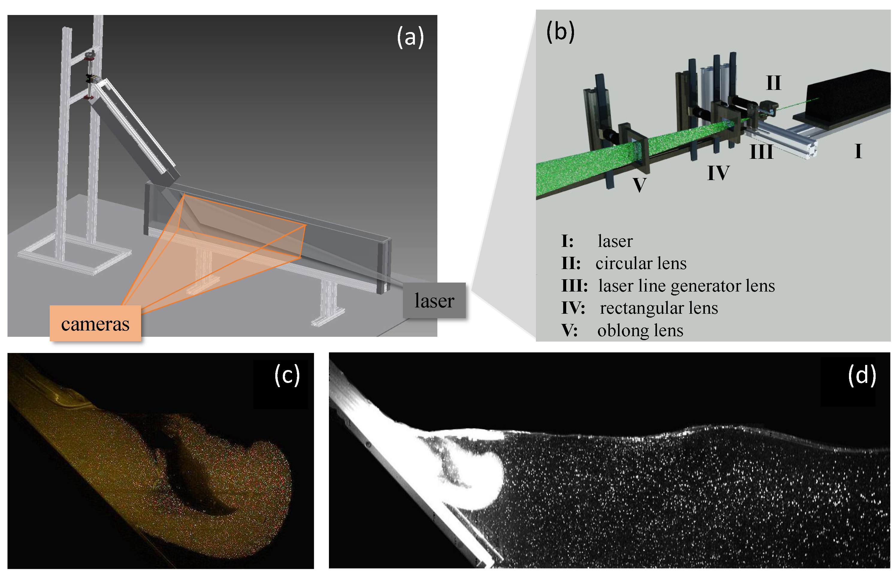
4.1. Facilities
4.2. Image Processing
5. Results
5.1. Empirical Equations for Predicting the Maximums of Wave Characteristics
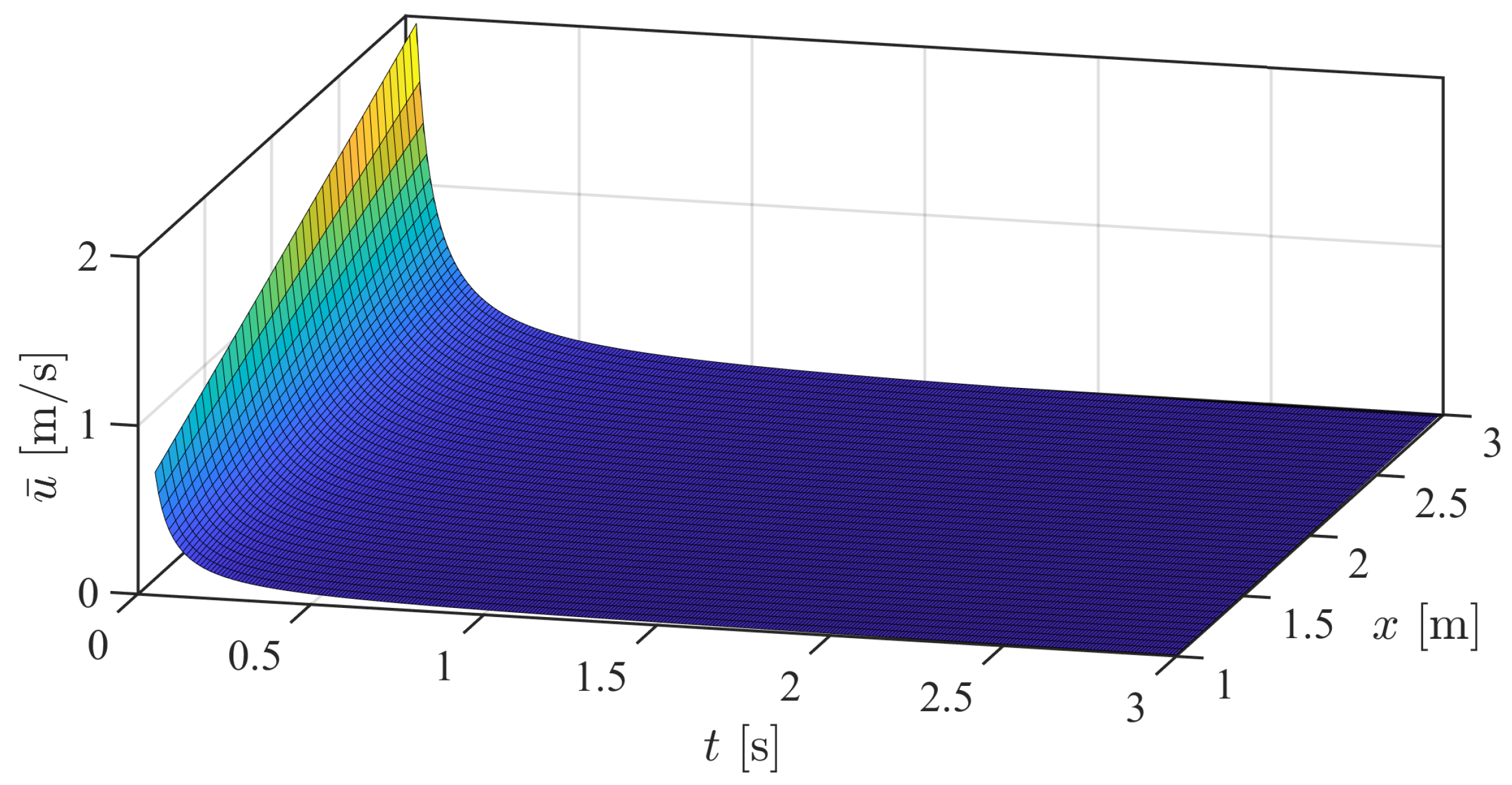
5.2. Time Series Data of the Slide Parameters Upon Impact
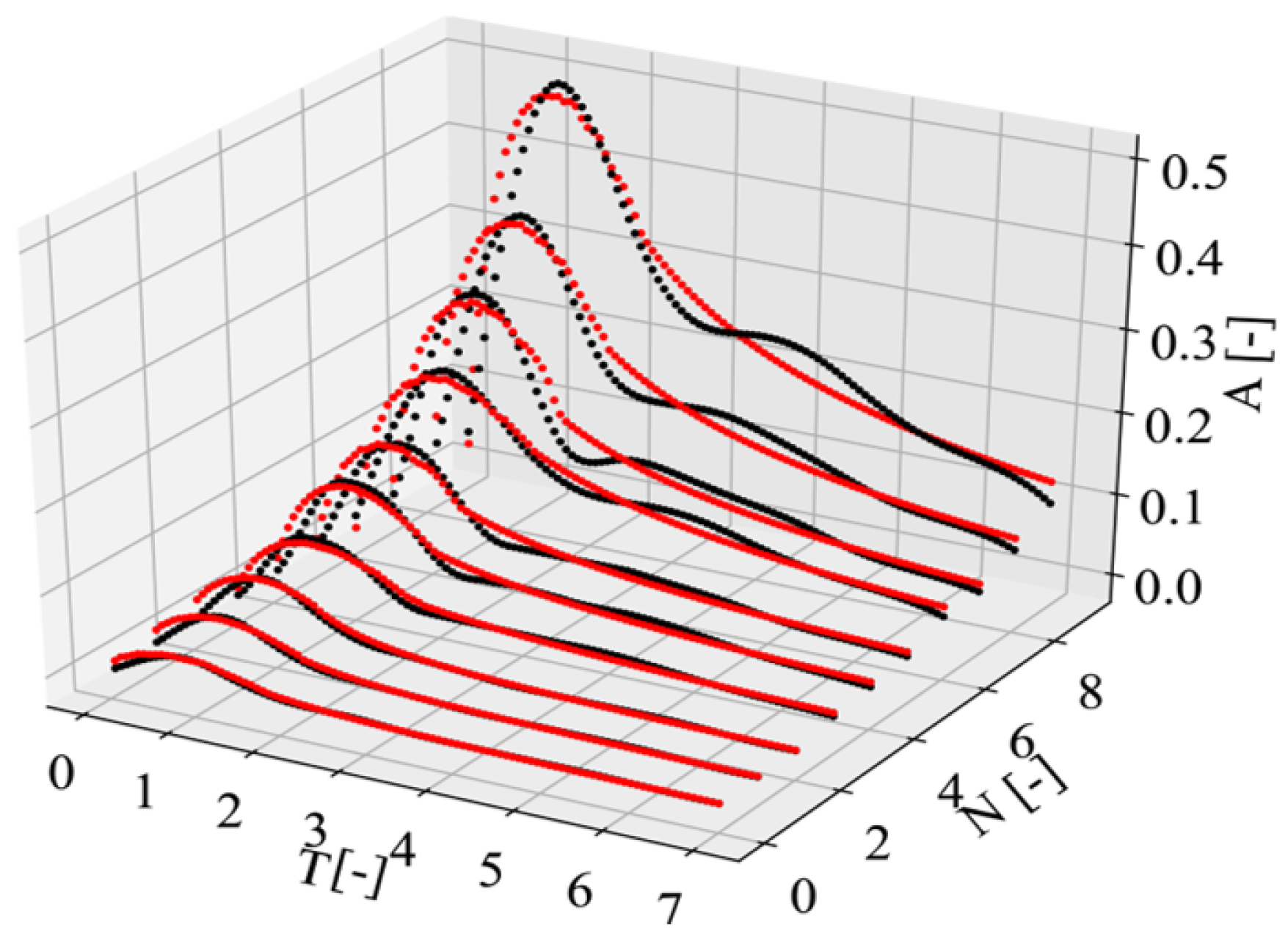
5.3. Prediction of the Temporal Wave Characteristics
6. Conclusions
Author Contributions
Funding
Institutional Review Board Statement
Informed Consent Statement
Data Availability Statement
Conflicts of Interest
References
- Gylfadóttir, S.S.; Kim, J.; Helgason, J.K.; Brynjólfsson, S.; Höskuldsson, Á.; Jóhannesson, T.; Harbitz, C.B.; Løvholt, F. The 2014 Lake Askja rockslide-induced tsunami: Optimization of numerical tsunami model using observed data. J. Geophys. Res. Ocean. 2017, 122, 4110–4122. [Google Scholar] [CrossRef]
- Gauthier, D.; Anderson, S.A.; Fritz, H.M.; Giachetti, T. Karrat Fjord (Greenland) tsunamigenic landslide of 17 June 2017: Initial 3D observations. Landslides 2018, 15, 327–332. [Google Scholar] [CrossRef]
- Ammann, W. Der Lawinenwinter 1999: Ereignisanalyse; Eidgenössisches Institut für Schnee-und Lawinenforschung: Zurich, Switzerland, 2000. [Google Scholar]
- Huber, A.; Hager, W. Forecasting impulse waves in reservoirs. In Proceedings of the Transactions of The International Congress on Large Dams, Florence, Italy, 26–30 May 1997; Volume 1, pp. 993–1006. [Google Scholar]
- Fritz, H.M. Initial Phase of Landslide Generated Impulse Waves. Ph.D. Thesis, ETH Zurich, Zurich, Switzerland, 2002. [Google Scholar]
- Panizzo, A.; De Girolamo, P.; Petaccia, A. Forecasting impulse waves generated by subaerial landslides. J. Geophys. Res. Ocean 2005, 110. [Google Scholar] [CrossRef]
- Zweifel, A. Impulswellen: Effekte der Rutschdichte und der Wassertiefe. Ph.D. Thesis, ETH Zurich, Zurich, Switzerland, 2004. [Google Scholar]
- Heller, V.; Bruggemann, M.; Spinneken, J.; Rogers, B.D. Composite modelling of subaerial landslide–tsunamis in different water body geometries and novel insight into slide and wave kinematics. Coast. Eng. 2016, 109, 20–41. [Google Scholar] [CrossRef]
- McFall, B.C.; Mohammed, F.; Fritz, H.M.; Liu, Y. Laboratory experiments on three-dimensional deformable granular landslides on planar and conical slopes. Landslides 2018, 15, 1713–1730. [Google Scholar] [CrossRef]
- Evers, F.; Heller, V.; Fuchs, H.; Hager, W.H.; Boes, R. Landslide-Generated Impulse Waves in Reservoirs: Basics and Computation; VAW-Mitteilungen: Zurich, Switzerland, 2019; Volume 254. [Google Scholar]
- Di Risio, M.; Sammarco, P. Analytical modeling of landslide-generated waves. J. Waterw. Port Coast. Ocean Eng. 2008, 134, 53–60. [Google Scholar] [CrossRef]
- Zitti, G.; Ancey, C.; Postacchini, M.; Brocchini, M. Impulse waves generated by snow avalanches: Momentum and energy transfer to a water body. J. Geophys. Res. Earth Surf. 2016, 121, 2399–2423. [Google Scholar] [CrossRef]
- Watts, P. Water Waves Generated by Underwater Landslides. Ph.D. Thesis, California Institute of Technology, Los Angeles, CA, USA, 1997. [Google Scholar]
- Abadie, S.; Morichon, D.; Grilli, S.; Glockner, S. Numerical simulation of waves generated by landslides using a multiple-fluid Navier–Stokes model. Coast. Eng. 2010, 57, 779–794. [Google Scholar] [CrossRef]
- Yavari-Ramshe, S.; Ataie-Ashtiani, B. Numerical modeling of subaerial and submarine landslide-generated tsunami waves-recent advances and future challenges. Landslides 2016, 13, 1325–1368. [Google Scholar] [CrossRef]
- Yavari-Ramshe, S.; Ataie-Ashtiani, B. A rigorous finite volume model to simulate subaerial and submarine landslide-generated waves. Landslides 2017, 14, 203–221. [Google Scholar] [CrossRef]
- Ruffini, G.; Heller, V.; Briganti, R. Numerical modelling of landslide-tsunami propagation in a wide range of idealised water body geometries. Coast. Eng. 2019, 153, 103518. [Google Scholar] [CrossRef]
- Fritz, H.M.; Hillaire, J.V.; Molière, E.; Wei, Y.; Mohammed, F. Twin tsunamis triggered by the 12 January 2010 Haiti earthquake. Pure Appl. Geophys. 2013, 170, 1463–1474. [Google Scholar] [CrossRef]
- Grilli, S.T.; Grilli, A.R.; David, E.; Coulet, C. Tsunami hazard assessment along the north shore of Hispaniola from far-and near-field Atlantic sources. Nat. Hazards 2016, 82, 777–810. [Google Scholar] [CrossRef]
- Engel, M.; Oetjen, J.; May, S.M.; Brückner, H. Tsunami deposits of the Caribbean Towards an improved coastal hazard assessment. Earth-Sci. Rev. 2016, 163, 260–296. [Google Scholar] [CrossRef]
- Poupardin, A.; Heinrich, P.; Frère, A.; Imbert, D.; Hébert, H.; Flouzat, M. The 1979 submarine landslide-generated tsunami in Mururoa, French Polynesia. Pure Appl. Geophys. 2017, 174, 3293–3311. [Google Scholar] [CrossRef]
- Kamphuis, J.; Bowering, R. Impulse waves generated by landslides. Coast. Eng. 1970, 575–588. [Google Scholar] [CrossRef]
- Zweifel, A.; Hager, W.H.; Minor, H.E. Plane impulse waves in reservoirs. J. Waterw. Port Coast. Ocean Eng. 2006, 132, 358–368. [Google Scholar] [CrossRef]
- Heller, V. Landslide Generated Impulse Waves: Prediction of Near Field Characteristics. Ph.D. Thesis, ETH Zurich, Zurich, Switzerland, 2007. [Google Scholar]
- Bullard, G.; Mulligan, R.; Carreira, A.; Take, W. Experimental analysis of tsunamis generated by the impact of landslides with high mobility. Coast. Eng. 2019, 152, 103538. [Google Scholar] [CrossRef]
- Bougouin, A.; Roche, O.; Paris, R.; Huppert, H.E. Experimental Insights on the Propagation of Fine-Grained Geophysical Flows Entering Water. J. Geophys. Res. Ocean. 2021, 126, e2020JC016838. [Google Scholar] [CrossRef]
- Meng, Z. Experimental study on impulse waves generated by a viscoplastic material at laboratory scale. Landslides 2018, 15, 1173–1182. [Google Scholar] [CrossRef]
- Meng, Z.; Ancey, C. The effects of slide cohesion on impulse-wave formation. Exp. Fluids 2019, 60, 151. [Google Scholar] [CrossRef]
- Meng, Z.; Hu, Y.; Ancey, C. Using a Data Driven Approach to Predict Waves Generated by Gravity Driven Mass Flows. Water 2020, 12, 600. [Google Scholar] [CrossRef]
- Hsiao, C. Panel data analysis—Advantages and challenges. Test 2007, 16, 1–22. [Google Scholar] [CrossRef]
- Hsiao, C. Analysis of Panel Data; Number 54 in 1; Cambridge University Press: Cambridge, UK, 2014. [Google Scholar]
- Arellano, M. Panel Data Econometrics; Oxford University Press: Oxford, UK, 2003. [Google Scholar]
- Hailemariam, A.; Smyth, R.; Zhang, X. Oil prices and economic policy uncertainty: Evidence from a nonparametric panel data model. Energy Econ. 2019, 83, 40–51. [Google Scholar] [CrossRef]
- Hu, Y.; Shao, C.; Gu, C.; Meng, Z. Concrete Dam Displacement Prediction Based on an ISODATA-GMM Clustering and Random Coefficient Model. Water 2019, 11, 714. [Google Scholar] [CrossRef]
- Cochard, S.; Ancey, C. Experimental investigation of the spreading of viscoplastic fluids on inclined planes. J. Non-Newton. Fluid Mech. 2009, 158, 73–84. [Google Scholar] [CrossRef]
- Ancey, C.; Andreini, N.; Epely-Chauvin, G. Viscoplastic dambreak waves: Review of simple computational approaches and comparison with experiments. Adv. Water Resour. 2012, 48, 79–91. [Google Scholar] [CrossRef]
- Fritz, H.; Hager, W.; Minor, H.E. Landslide generated impulse waves: 2 Hydrodynamic impact craters. Exp. Fluids 2003, 35, 520–532. [Google Scholar] [CrossRef]
- Mohammed, F.; Fritz, H.M. Physical modeling of tsunamis generated by three-dimensional deformable granular landslides. J. Geophys. Res. Ocean 2012, 117. [Google Scholar] [CrossRef]
- Heller, V.; Spinneken, J. On the effect of the water body geometry on landslide-tsunamis: Physical insight from laboratory tests and 2D to 3D wave parameter transformation. Coast. Eng. 2015, 104, 113–134. [Google Scholar] [CrossRef]
- Walder, J.S.; Watts, P.; Sorensen, O.E.; Janssen, K. Tsunamis generated by subaerial mass flows. J. Geophys. Res. Solid Earth 2003, 108. [Google Scholar] [CrossRef]
- Fernández-Nieto, E.D.; Bouchut, F.; Bresch, D.; Diaz, M.C.; Mangeney, A. A new Savage–Hutter type model for submarine avalanches and generated tsunami. J. Comput. Phys. 2008, 227, 7720–7754. [Google Scholar] [CrossRef]
- Zitti, G.; Ancey, C.; Postacchini, M.; Brocchini, M. Snow avalanches striking water basins: Behaviour of the avalanche’s centre of mass and front. Nat. Hazards 2017, 88, 1297–1323. [Google Scholar] [CrossRef]
- Swamy, P.A. Efficient inference in a random coefficient regression model. Econom. J. Econom. Soc. 1970, 38, 311–323. [Google Scholar] [CrossRef]
- Balmforth, N.; Craster, R.; Perona, P.; Rust, A.; Sassi, R. Viscoplastic dam breaks and the Bostwick consistometer. J. Non-Newton. Fluid Mech. 2007, 142, 63–78. [Google Scholar] [CrossRef]
- Bonn, D.; Denn, M.M.; Berthier, L.; Divoux, T.; Manneville, S. Yield stress materials in soft condensed matter. Rev. Mod. Phys. 2017, 89, 035005. [Google Scholar] [CrossRef]
- Müller, A.; Dreyer, M.; Andreini, N.; Avellan, F. Draft tube discharge fluctuation during self-sustained pressure surge: Fluorescent particle image velocimetry in two-phase flow. Exp. Fluids 2013, 54, 1514. [Google Scholar] [CrossRef]
- Heller, V.; Hager, W.H. Impulse product parameter in landslide generated impulse waves. J. Waterw. Port Coast. Ocean Eng. 2010, 136, 145–155. [Google Scholar] [CrossRef]


| Test | c [%] | [m] | [-] | [kg] | [m] |
|---|---|---|---|---|---|
| T1 | 2.0 | 1.05 | 3.0 | 0.2 | |
| T2 | 2.0 | 0.95 | 3.5 | 0.2 | |
| T3 | 2.0 | 0.85 | 4.0 | 0.2 | |
| T4 | 2.0 | 0.85 | 4.5 | 0.2 |
| Nbr | MSE | MSE | ||
|---|---|---|---|---|
| 1 | 0.927 | 0.327 | 0.889 | 0.402 |
| 2 | 0.934 | 0.273 | 0.924 | 0.292 |
| 3 | 0.939 | 0.196 | 0.894 | 0.205 |
| 4 | 0.928 | 0.464 | 0.914 | 0.506 |
| 5 | 0.929 | 0.135 | 0.929 | 0.136 |
| 6 | 0.931 | 1.490 | 0.905 | 1.549 |
| 8 | 0.873 | 1.048 | 0.891 | 1.177 |
| 9 | 0.937 | 0.643 | 0.930 | 0.680 |
| 10 | 0.923 | 0.543 | 0.916 | 0.566 |
Disclaimer/Publisher’s Note: The statements, opinions and data contained in all publications are solely those of the individual author(s) and contributor(s) and not of MDPI and/or the editor(s). MDPI and/or the editor(s) disclaim responsibility for any injury to people or property resulting from any ideas, methods, instructions or products referred to in the content. |
© 2023 by the authors. Licensee MDPI, Basel, Switzerland. This article is an open access article distributed under the terms and conditions of the Creative Commons Attribution (CC BY) license (https://creativecommons.org/licenses/by/4.0/).
Share and Cite
Meng, Z.; Zhang, J.; Hu, Y.; Ancey, C. Temporal Prediction of Landslide-Generated Waves Using a Theoretical–Statistical Combined Method. J. Mar. Sci. Eng. 2023, 11, 1151. https://doi.org/10.3390/jmse11061151
Meng Z, Zhang J, Hu Y, Ancey C. Temporal Prediction of Landslide-Generated Waves Using a Theoretical–Statistical Combined Method. Journal of Marine Science and Engineering. 2023; 11(6):1151. https://doi.org/10.3390/jmse11061151
Chicago/Turabian StyleMeng, Zhenzhu, Jinxin Zhang, Yating Hu, and Christophe Ancey. 2023. "Temporal Prediction of Landslide-Generated Waves Using a Theoretical–Statistical Combined Method" Journal of Marine Science and Engineering 11, no. 6: 1151. https://doi.org/10.3390/jmse11061151
APA StyleMeng, Z., Zhang, J., Hu, Y., & Ancey, C. (2023). Temporal Prediction of Landslide-Generated Waves Using a Theoretical–Statistical Combined Method. Journal of Marine Science and Engineering, 11(6), 1151. https://doi.org/10.3390/jmse11061151