A Hybrid Excitation Model Based Lightweight Siamese Network for Underwater Vehicle Object Tracking Missions

Abstract

Performing object tracking tasks and efficiently perceiving the underwater environment in real time for underwater vehicles is a challenging task due to the complex nature of the underwater environment. A hybrid excitation model based lightweight Siamese network is proposed to solve the mismatch between underwater objects with limited characteristics and complex deep learning models. The lightweight neural network is applied to the residual network in the Siamese network to reduce the computational complexity and cost of the model while constructing a deeper network. In addition, to deal with the changeable complex underwater environment and consider the timing of video tracking, the global excitation model (HE module) is introduced. The model adopts the excitation methods of space, channel, and motion to improve the accuracy of the algorithm. Based on the designed underwater vehicle, the underwater target tracking and target grabbing experiments are carried out, and the experimental results show that the proposed tracking algorithm has a high tracking success rate.

1. Introduction

Real-time and efficient perception of the underwater environment is required for underwater vehicles to adapt to the complex underwater environment. The accuracy of perception is related to the autonomous operation accuracy of underwater vehicles to a large extent. Target tracking is one of the important links in the autonomous perception of the underwater environment, and it is also one of the most basic and challenging research topics in the field of computer vision. Vision-based motion object tracking has been widely used in surveillance systems, UAV vision systems, military reconnaissance, human–computer interaction, and unmanned vehicles [1]. In the field of underwater operations, tracking vessels, obstacles, and mines are crucial for normal maritime operations [2,3]. In short, underwater vehicles collect videos by carrying cameras on the vehicle units. The target to be tracked is determined by the rectangular box given in the first frame of the video. Underwater target tracking is achieved by tracking the target in subsequent frames, assisting the underwater robot in completing its task. The complex underwater environment and the motion of the target interfere with underwater vehicle target tracking. Therefore, the choice of tracking method is crucial.

Several investigations of visual tracking have been proposed in recent years [4,5], and most of the state-of-the-art approaches are based on correlation filters or deep learning. Some trackers combine multiple methods to improve tracking performance. In recent years, with the high development of deep learning, it has had a wide range of applications in the field of object detection as well as object tracking because of the powerful representation capability of depth features for objects. Boosting and KCF are classic object-tracking methods in underwater environments. The KCF [6] method introduces kernel function and achieves very good results. Its tracking speed is very fast and greatly improved. Boosting Tracker is an online version of AdaBoost [7]. It is based on the Haar cascade face detector. It classifies the pixels around the previous result, uses the highest score as the result, and updates it through additional data. However, the above method is prone to tracking drift when multiple targets appear densely and close to each other.

The deep learning method has many applications in underwater vehicle object tracking missions. Li et al. proposed the SiamRPN++ [8] target tracking algorithm, which uses a spatial sensing strategy to process data. Zhang et al. proposed the DaSiamRPN [9] method to improve the generalization ability of the network through data expansion, and used the motion direction fuzzy method to improve the discrimination ability of the tracking. Many other methods have made contributions, such as CFNet [10], GradNet [11], DeepSRDCF [12], STRCF [13], Staple [14], Mixformer [15] and OSTrack-384 [16].

In addition, some tracking methods have been proposed for specific underwater objects. The article [17,18] proposed an underwater cable visual tracking system, which integrates the information collected by optical vision and acoustic vision to locate and track the cable. The article [19,20] proposed improved algorithms based on YOLOv4 to detect and track underwater organisms and multi-ship targets. Ye et al. [21] proposed a Bayesian-Transformer Neural Network to complete the ship target identification task using track information.

Although deep learning-based approaches have been used in underwater environments, they have not been able to solve some problems in practice, such as (1) when operating underwater, multiple targets can densely appear and be close to each other, leading to occlusion of the targets; (2) the underwater vehicle’s own components, such as claws and cables, can also cause occlusion of the target, affecting the operational effectiveness; and (3) the number of underwater samples is relatively small, with limited features. To address these issues and improve the speed and robustness of deep learning methods, a novel lightweight unified network tracking method has been proposed.

The main contributions of the proposed algorithm are as follows:

(1)

To solve the problem of the deep learning models that have become increasingly complex as their performance improves, a lightweight network is introduced. Lightweight neural networks are structures that extract the same number of features as regular convolutions but with fewer parameters. The use of lightweight networks reduces the parameter size and computational complexity of the network. This method maintains accuracy, improves temporal aspects, and reduces the computational complexity and cost of the model.

(2)

To enhance the learning and understanding capabilities of the algorithm for the target, we have introduced a mixed excitation model. The mixed excitation model consists of three components: the spatial excitation method for extracting the temporal and spatial relationships of the target, the channel excitation method for extracting weights between different channels, and the motion excitation method for extracting the trajectory relationship of the target between adjacent frames. These pieces of information are combined and applied to the feature extraction network. Multidimensional and comprehensive extraction of target features improves the performance of the algorithm.

(3)

Aiming at the problem of easy occlusion in an underwater environment, an adaptive strategy is designed. In addition to ensuring the training accuracy, the complex positive sample is added to make the training more targeted. Due to the presence of water resistance, the movement speed of underwater targets is much slower compared to aerial targets. Considering this difference, a new tracking strategy is proposed to narrow down the tracking range and improve the robustness of the algorithm. The tracking strategy based on underwater environmental characteristics improves the algorithm’s success rate in underwater environments, ensuring good tracking performance even in scenarios with limited visibility and turbid water conditions.

We tested the performance of the algorithm on both underwater datasets and publicly available datasets. The algorithm demonstrates a reduction in parameter count and computational complexity compared to other deep learning algorithms. It shows good tracking results in underwater environments with challenges such as turbid water and limited visibility. Experimental results show further improvements in performance on underwater datasets and perform well on public datasets, demonstrating the algorithm’s comprehensive tracking capabilities.

The remainder of this article is organized as follows: Section 2 proposes autonomous control and target tracking architecture used for the underwater vehicle experiment. In Section 3, the backbone network used by the algorithm is explained in detail, including SiamRPN, a lightweight network improved for neural networks with many parameters such as residual network and mixed excitation model. In Section 4, the SL-HENet underwater vehicle object tracking algorithm is proposed. In Section 5, experiments are arranged to verify the advancement of the algorithm, SL-HENet is compared with other similar algorithms, and the advantages of the algorithm are analyzed. Section 6 presents the conclusions and future research directions.

2. Autonomous Control and Target Tracking Architecture for Underwater Vehicles

To realize target detection and object tracking missions, the autonomous architecture has been designed based on an underwater vehicle embedded system (see Figure 1).

The architecture is composed of four function modules: localization module, automatic planning and reasoning module, control module, and target perception module which includes target detection and visual tracking algorithm. The subsystem of the module runs with an independent task schedule and a unified communication protocol.

The underwater vehicle collects video information in real time through its cameras. The perception module will realize target perception and visual tracking through the SL-HENet tracking algorithm proposed in this paper. This module can realize visual tracking throughout the images and help the controller module keep the target in sight. The localization module will provide the vehicle position information through dead reckoning from three-dimensional velocities and angular information from the Doppler Velocity Log (DVL) and magnetic compass. This module can help the vehicle complete the target tracking control process. With control modules, the vehicle can keep the target in line of sight, controlling the vehicle’s speed and position.

3. Backbone Network Structure

3.1. SiamRPN

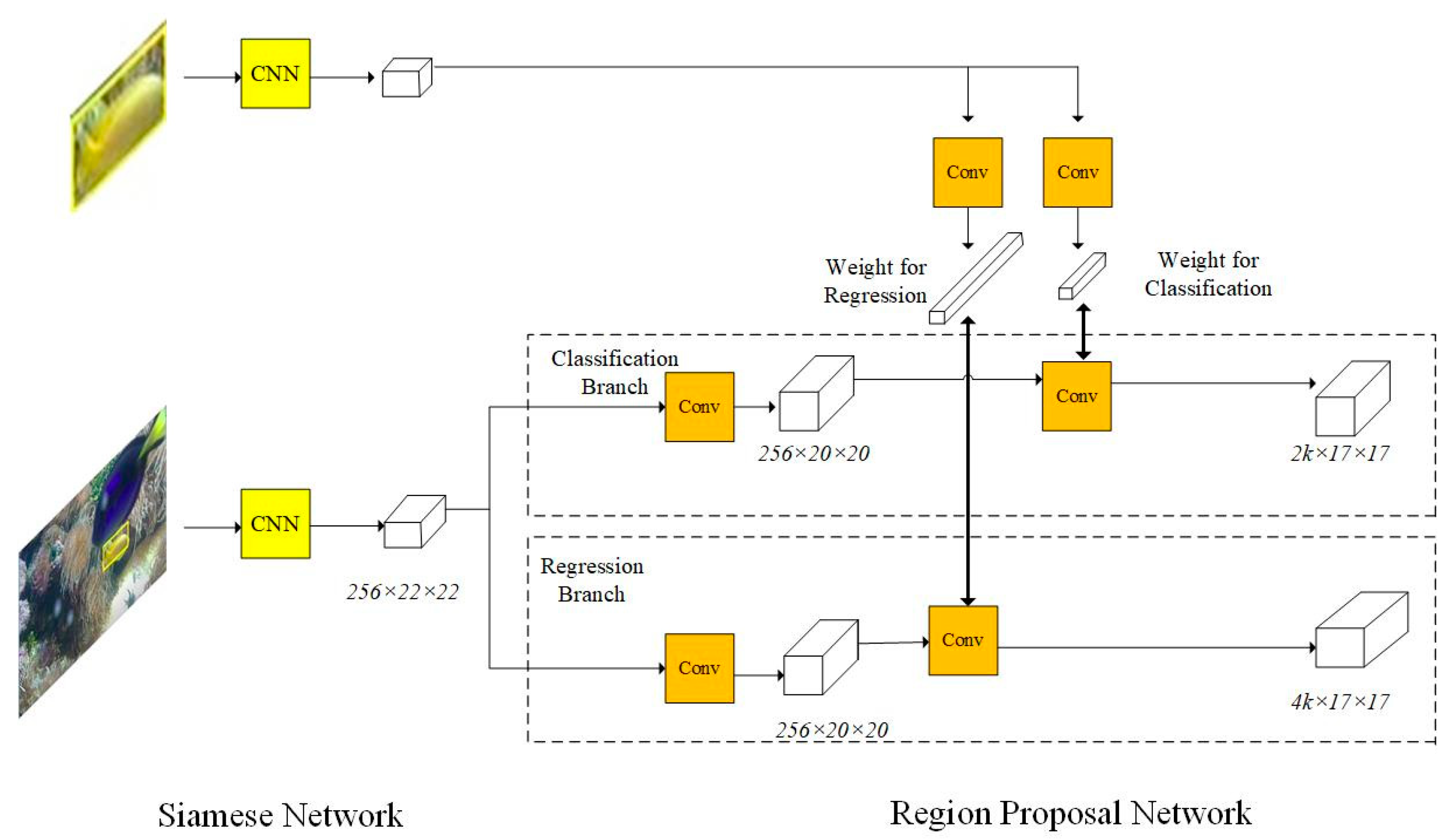
The methodology, High Performance Visual Tracking with Siamese Region Proposal Network, was proposed in 2018 [22]. The whole tracking framework is composed of a Siamese network and a region proposal network. The structure is shown in Figure 2. The left side of Figure 2 is a Siamese network for feature extraction. The region proposal network is located in the middle and has two branches, one for classification and the other for regression. Pairwise correlation is used to obtain the output of the two branches. The information on the two output feature maps is located on the right. In the classification branch, the output feature map has 2K channels, which correspond to the foreground and background of K anchors. In the regression branch, the output feature map has 4K channels corresponding to the four coordinates of the proposed refinement for K anchors.

In the Siamese network, the full convolution structure without filling is adopted. The Siamese network used to extract image features is divided into two branches: the template branch and the detection branch. The small image receiving the template frame is the template branch, and the image receiving the current frame is the detection branch. Only the inputs of the two networks are different, and the weight parameters are the same. The region proposal network was first proposed in fast R-CNN. Before the region proposal network, the traditional extraction methods were very time-consuming, and these methods are not enough for detection. The enumeration of multiple anchors, such as region proposal network and sharing convolution features, make the extraction method obtain high quality and have time efficiency. Due to the supervision of foreground, background classification, and bounding box regression, RPN can be extracted more accurately. There are several fast R-CNN [23] variants using RPN, such as R-FCN considering the location information of components and FPN [24] using feature pyramid networks to improve the performance of small object detection. Region proposal networks have many successful applications in detection because of their high speed and excellent performance. The region proposal network is divided into two branches: the classification branch and the regression branch. The classification branch is used to distinguish the foreground and background in the picture. The regression branch is used for coordinate regression to make the position and size of the tracking box more accurate.

3.2. Residual Network Structure

The depth of the network is crucial to the performance of the model. He et al. [18] found in the experiment that when the number of network layers increases to a certain extent, the network accuracy will be saturated or even decline, and it is not a problem caused by overfitting. Therefore, the residual network is generated. For a pile base structure, when the input is $x$, the learned characteristics are recorded as $H\left(x\right)$. We expect to learn the residuals.

$$F\left(x\right)=H\left(x\right)-x$$

(1)

Therefore, the original learning characteristic is

$$F\left(x\right)+x$$

(2)

The residual learning is easier than the original feature learning, and the actual residual will not be zero, which enables the heap base to learn new features based on the input features; thus, it has better performance.

3.3. Lightweight Neural Network Model

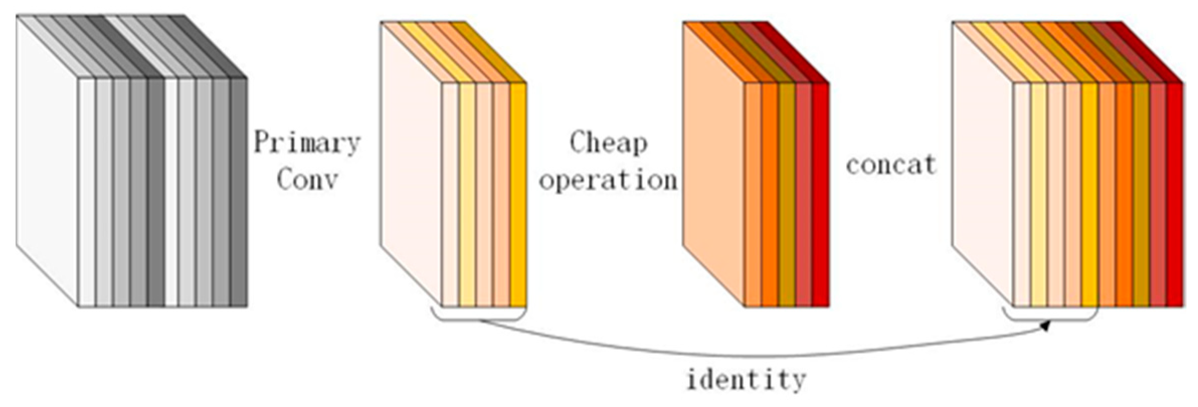
Ordinary convolutional neural networks generate rich feature maps, but for deep neural networks such as residual networks, the number of parameters can be significant, leading to increased computational costs. While these models offer high performance, their large computational requirements can limit their applicability in underwater environments. A lightweight neural network is a structure that extracts the same number of features as a regular convolutional network but with fewer parameters. Figure 3 illustrates the architecture of the lightweight neural network model. A small number of convolutional kernels are used to extract a part of the features from the input in the lightweight neural network. Then, the generated features are linearly transformed layer by layer to obtain another portion of the features. Finally, the two sets of feature maps are concatenated to generate the final feature map. The same number of feature maps as regular convolutions are generated with lower computational costs.

Suppose that the size of the input characteristic graph is $h\times w\times t$, the size of the output characteristic graph is $h^{\prime }\times w^{\prime }\times m$, and the size of the convolution kernel is $k\times k$. In the soap operation transformation, we assume that the channel of the characteristic graph is $c$, the number of transformations is $n$, the average kernel size of each linear operation is $z\times z$, and the number of new characteristic graphs is m, then we can obtain the equation:

$$m=n\times c$$

(3)

Since there is an identity transformation at the end of the transformation process, the actual effective transformation quantity is $n-1$. Therefore, the following formula can be obtained from the above formula:

$$c\times \left(n-1\right)=\frac{m}{n}\times \left(n-1\right)$$

(4)

where the size of $d\times d$ is similar to that of $k\times k$, and $n\ll t$; thus, the theoretical acceleration ratio can be calculated as:

$$\begin{array}{l}{{\displaystyle r}}_n=\frac{m·h^{\prime }·w^{\prime }·t·k·k}{\frac{m}{n}·h^{\prime }·w^{\prime }·t·k·k+(n-1)\frac{m}{n}·h^{\prime }·w^{\prime }·z·z}\\ =\frac{t·k·k}{\frac{1}{n}·t·k·k+\frac{n-1}{n}z·z}\\ \approx \frac{n·t}{n+t-1}\\ \approx n\end{array}$$

(5)

The compression ratio of the calculation model is:

$$r_t=\frac{m·t·k·k}{\frac{n}{m}·t·k·k+\left(n-1\right)·z·z}\approx \frac{n·t}{n+t-1}\approx n$$

(6)

Therefore, theoretically, the speed of the model is improved and the parameters are reduced as a whole.

We calculated and compared the computational and parameter quantities of the network before applying lightweight techniques.

Table 1. Comparison of the amount of computation and parameters of the network.

Model	FLOPs	Weights
ResNet-50	6.51 G	33.74 M
Versatile-ResNet-50	6.03 G	30.92 M
Thinet-ResNet-50	5.79 G	25.65 M
Ours	4.46 G	24.97 M

shows the comparison between the basic feature extraction network ResNet-50 and other models that reduce network complexity with the proposed algorithm. The FLOPs (floating point operations) represent the computational complexity of the model and the Weights represent the number of model parameters. As can be seen from the table, compared with the basic network model, the proposed algorithm reduces the computational complexity by 2.05 G, a 31.4% reduction, and reduces the model parameters by 26%, with 24.97 M parameters compared to the basic network’s 33.74 M. Moreover, it also shows a decrease compared to other models.

3.4. Mixed Excitation Model

3.4.1. Spatial Excitation Method

As shown in Figure 4, the structure of the spatial temporal excitation method is similar to that of the SE net [25]. By making a global average pool for all channels and introducing a single channel 3 × 3 × 3 3D convolution, it is possible to obtain a spatial temporal attention image with a very small amount of computation and increase the connection between successive video frames. The attention image is then dot multiplied by the input features to obtain the corresponding features excited by spatial temporal information.

3.4.2. Channel Excitation Method

The channel excitation method is based on the SE block of the SE net. Since the video action contains timing information, 1D convolution in the time domain is inserted between channel compression and decompression to enhance the interdependence of channels in the time domain. Similar to SE, you can obtain an attention map based on the channel. The global spatial information of the input feature is obtained by spatial average pooling and then is used 1 × 1 convolution to compress the number of channels of F (the compression multiple in this paper is 16) to obtain the compressed characteristic fr, adjust the size of FR to obtain fr′, and then obtain the output after three-dimensional one-dimensional convolution. The structure is shown in Figure 5.

3.4.3. Motion Excitation Method

This mainly describes the movement of actions between each adjacent two frames. Similar to the frame difference method, the previous frame is related to the next one. The motion information is modeled based on the feature level rather than the pixel level. First, expand in the timing latitude, carry out 2D convolution, respectively, and then combine the structure. The structure is shown in Figure 6.

3.4.4. HE-Module Network Model

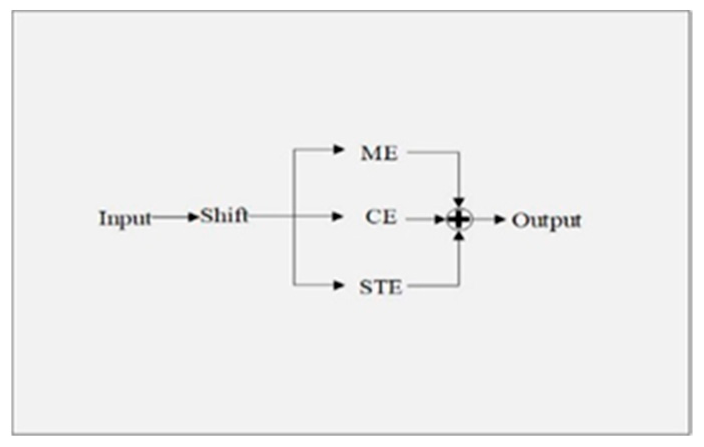
The HE-Module is a hybrid attention mechanism combining space, channel, and motion excitation methods. It can effectively process multiple types of information on the feature layer in a single network by using multipath excitation. The combination of spatiotemporal features and motion features can be similarly understood as a dual flow structure but modeling the motion within the network based on the feature level instead of generating another type of input to train the network, which greatly reduces the amount of calculation and can also extract the global feature information between fused video frames. It is very helpful for underwater video object-tracking missions. The structure is shown in Figure 7.

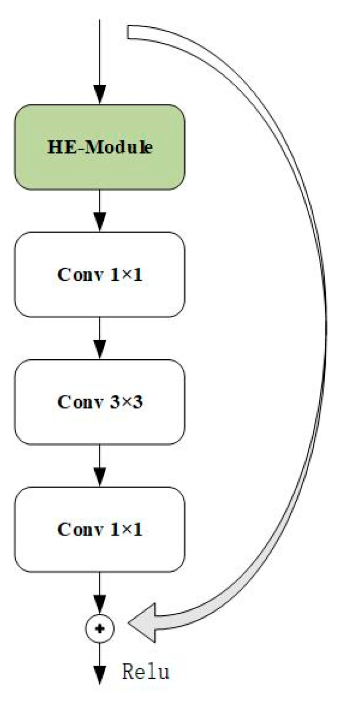
The HE-Module can be flexibly inserted into the network architecture of various visual problems. This paper puts the HE-Module into the residual block of the residual network to improve the generalization performance of network training. The structure of the residual block is shown in Figure 8.

4. SL-HENet Underwater Vehicle Object Tracking Algorithm

In this section, we will provide a detailed introduction to the algorithm from four aspects: the Siamese network tracking framework, the SL-HENet framework, the tracking strategy based on the influence of sea currents, and the strategy of adaptive training.

4.1. Siamese Network Tracking Framework

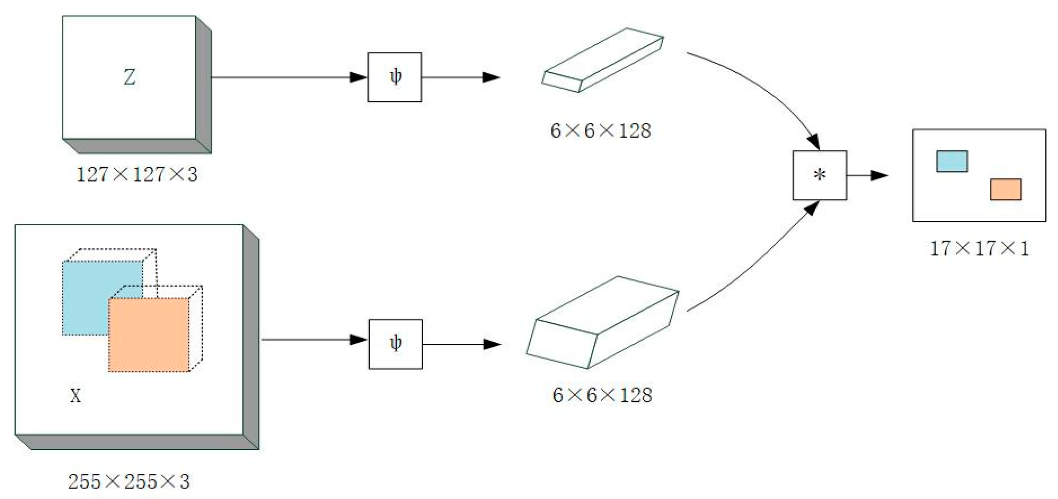
With the proposal of a full convolution Siamese network [26], the tracking model based on the Siamese neural network has become a hot spot in the field of object tracking. Figure 9 is a schematic diagram of the SiamFC network model. The algorithm only uses the object of the first frame to learn the appearance model and trains a similarity-matching function. The subsequent frames calculate the similarity with the model of the first frame to find the maximum response position of the target.

4.2. SL-HENet Framework

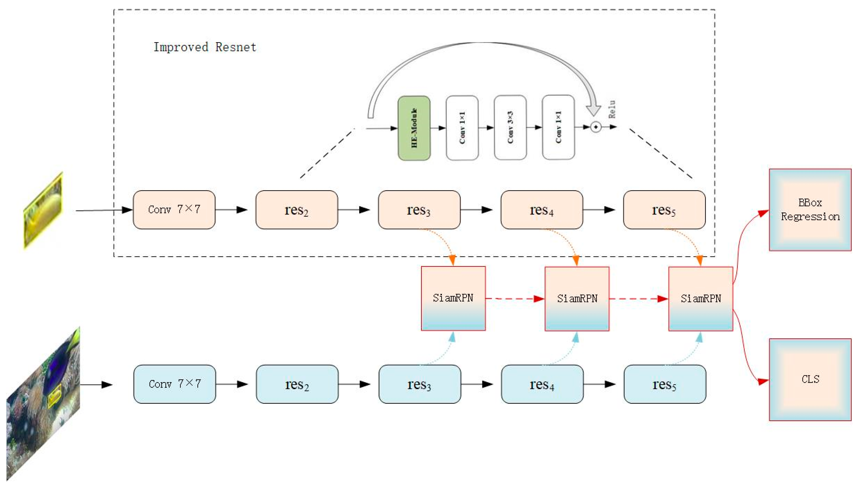
The above sections introduce the details of the object tracking backbone network structure and the Siamese network tracking framework. The Siamese network is widely used in tracking, with good performance and real-time performance. While constructing a deep neural network, a light neural network can reduce the amount of calculation, reduce the burden of underwater application of the model, and enhance the generalization performance. The global feature model combines spatial excitation, channel excitation, and motion excitation, extracts the feature association between video frames, integrates the global information, and is applied in the backbone network to improve performance. Based on the above three points, the SL-HENet tracking method in this paper is proposed, and the novel network structure is shown in Figure 10.

The backbone network of the algorithm is the Siamese network, and the feature extraction network is an improved residual learning network based on a mixed excitation model. The algorithm consists of five groups of convolutional operations. The first group of convolution includes only one convolution computation. The residual blocks in the following four groups of convolutional operations all adopt modified residual blocks based on a hybrid activation model. The outputs obtained from the last three groups of convolutional operations in the residual network are passed as inputs to three SiamRPN blocks. Since the outputs of the three SiamRPN blocks have the same size, a weighted sum is directly computed on the obtained outputs:

$$S={\displaystyle \sum _{j=3}^5{{\displaystyle \alpha }}_i}\ast {{\displaystyle S}}_j,B={\displaystyle \sum _{j=3}^5{{\displaystyle \beta }}_i{{\displaystyle B}}_j}$$

(7)

where $S$ represents the weighted sum of the classification output, $S_j$ represents the output of the j group of convolutions, B represents the weighted sum of the bounding box regression branch output, and $B_j$ represents the bounding box regression output of the j group of convolutional operations.

The template frame and subsequent matching frames are input into the Siamese network. Through the improved residual network, the output of each residual block is obtained. Then, these outputs are individually passed into the SiamRPN model to obtain the classification and regression results for each residual block. A weighted average is performed on these results to obtain the final tracking result.

4.3. Tracking Strategy Based on the Influence of Sea Currents

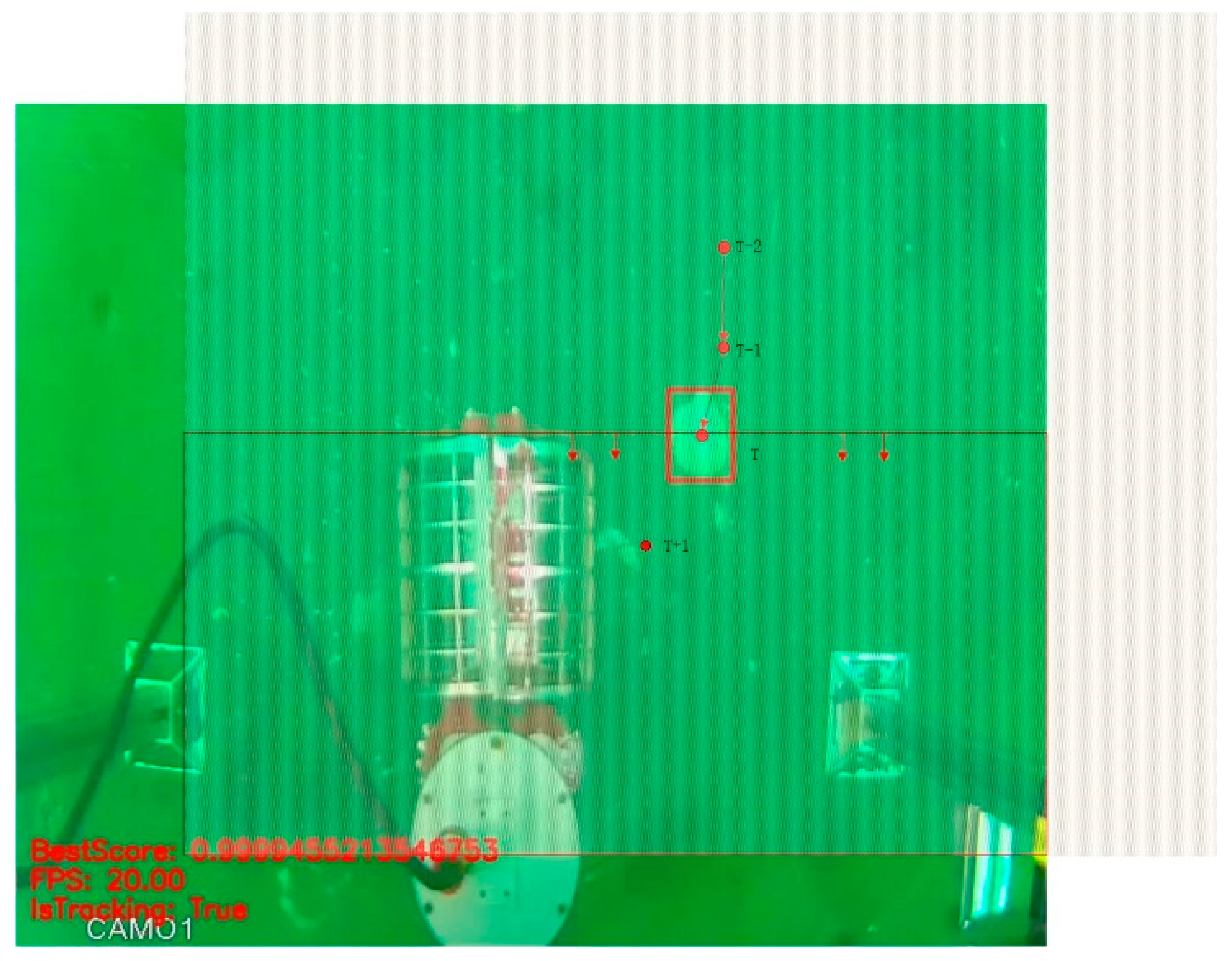
In the actual underwater environment, there is a common presence of currents, which can have different effects on different underwater environments. Especially for sandy seafloor, there are currents caused by the movement of underwater objects or caused by the natural flow of seawater that will bring up sand, which may cause a line-of-sight obstruction to the underwater camera or cause the target to be completely covered by sand. Moreover, due to the underwater resistance, the speed of the underwater target when moving will be much slower than that of the target in the air. According to these situations, this paper proposes a novel tracking strategy to narrow the tracking range and improve the robustness of the algorithm. The process is shown in Figure 11. The specific procedure is as follows.

After determining the tracking result of the previous frame, the coordinates of the center point of the tracking frame (cx, cy) are used as the base and filled outward to the size of the original image, and the coordinates of the top left point of the expanded image are cx − w/2 and cy − h/2, and the coordinates of the bottom right point are cx + w/2 and cy + h/2. The overlap between the original and the expanded image is set as the selection range for the next frame of the tracking object. This operation takes advantage of the above-mentioned characteristics to reduce unnecessary operations and incorrect tracking during underwater vehicle object tracking and improves the robustness of the method.

4.4. The Strategy of Adaptive Training

There is a serious occlusion problem in underwater tasks, which is also a problem to be solved in the field of object tracking. Based on the consideration of occlusion in underwater vehicle object tracking missions, a novel adaptive training strategy is proposed to solve the impact of occlusion on underwater tracking tasks. The underwater dataset is input into the model for training. After the training, the test is carried out to obtain the test results. Several frames with good performance in the results are intercepted. The obtained results are occluded in random directions and sizes. Finally, the occluded image is added to the second training in the dataset. The training strategy in this paper not only ensures the training accuracy but also increases the complex positive samples of occlusion, which makes the training more targeted.

5. Experiments

5.1. Details of Algorithm Implementation

The algorithm implementation and debugging of this paper are based on Ubuntu 16.04 operating system, the computer hardware is configured as Intel Core i7-8700k, the main frequency is 3.7 GHz and GeForce RTX1080ti graphics card. This algorithm is trained on ILSVRC2015 [27] and underwater dataset video sequences, respectively. The ILSVRC2015 dataset has a variety of video target objects and has certain universality. Underwater datasets collect datasets with certain underwater environmental characteristics for themselves. The proposed algorithm was compared with the commonly used tracking algorithm on the OTB100 dataset [28] and the VOT2016 dataset [29]. In this paper, the random gradient descent optimization algorithm is used to train the network with the momentum parameter of 0.9. The learning rate decreases gradually from 10⁻⁸ to 10⁻³ in the training process. The parameters are initialized with the Gaussian function and the batch size is set to 16.

5.2. Analysis of Experimental Results

The underwater vehicle tracks the target after identifying it in the pool. Figure 12 illustrates the depth variations during the target tracking process of the underwater robot. The changes in the Z-axis coordinate refer to the height variations of the vehicle relative to the seabed. The acquisition of underwater video data relies on the movement of the underwater vehicle. Multiple videos are collected. The videos are intercepted according to the setting of 7–10 pictures per frame, and a total of 4757 images are collected. Using this underwater dataset for tracking tests, it is concluded that the accuracy of this algorithm is 76.3%.

To validate the effectiveness of the lightweight network, the mixed excitation model, and tracking strategies, we compared the Siamese network tracking algorithms based on deep learning called Siam, tracking algorithms incorporating the lightweight network called SiamLW, and the SL-HENet underwater vehicle object tracking algorithm on the publicly available OTB100 dataset. The success rate and accuracy of tracking are shown in

Table 2. Comparison of algorithms after introducing different models.

Tracker Name	Success Rate	Accuracy
Siam	65.40%	87.40%
SiamLW	66.40%	87.90%
SL-HENet	69.10%	90.80%

. It can be observed that with the introduction of the lightweight networks, the mixed excitation model, and tracking strategies, the success rate and accuracy of the tracking algorithm gradually improve, validating the effectiveness of the algorithm.

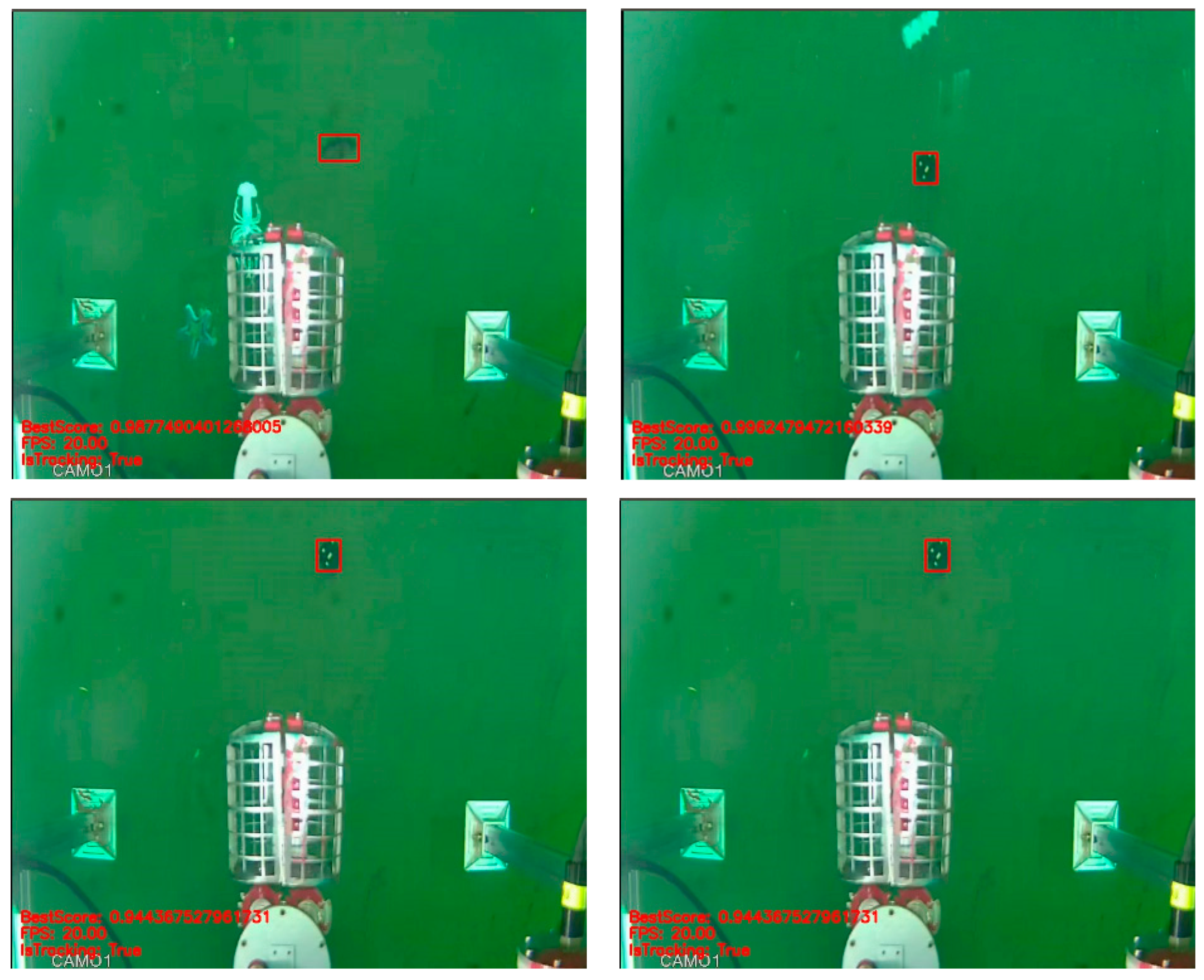
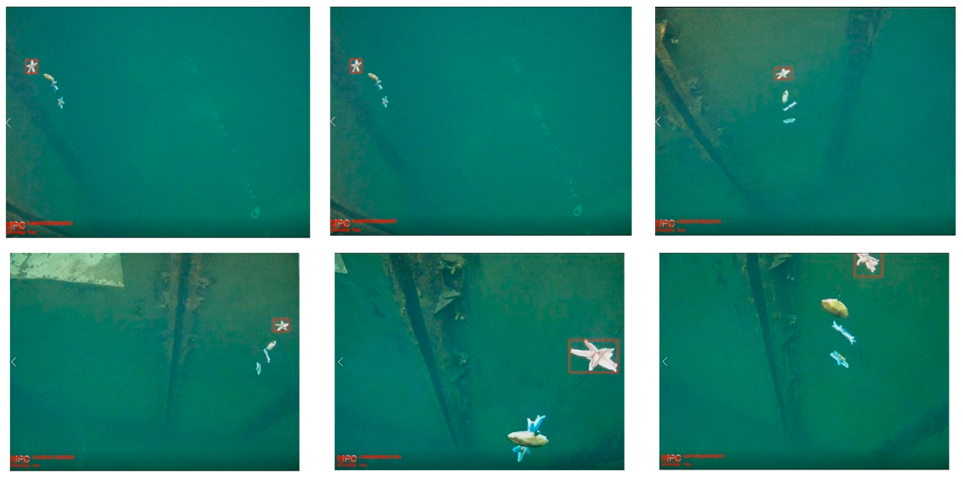
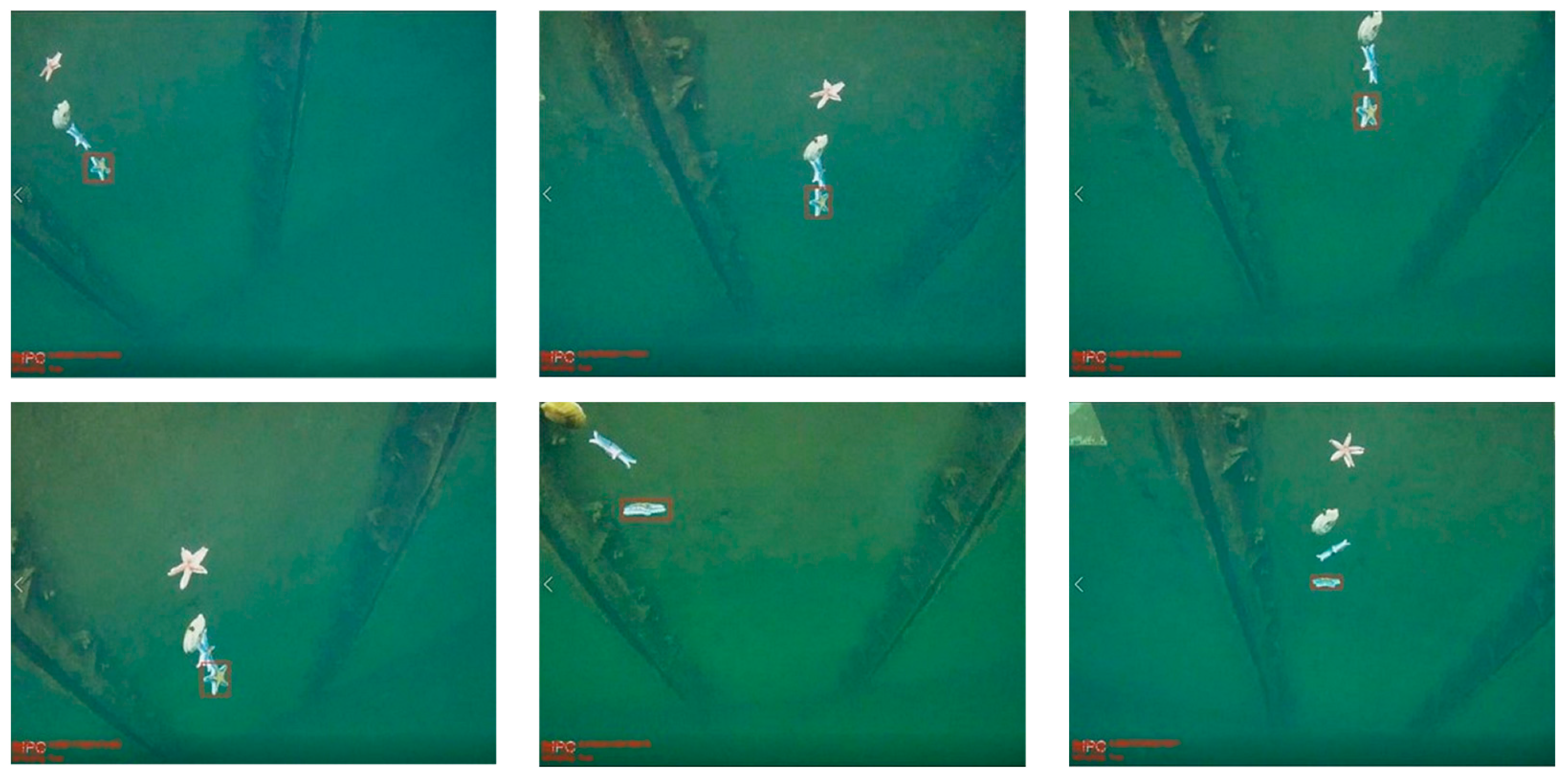
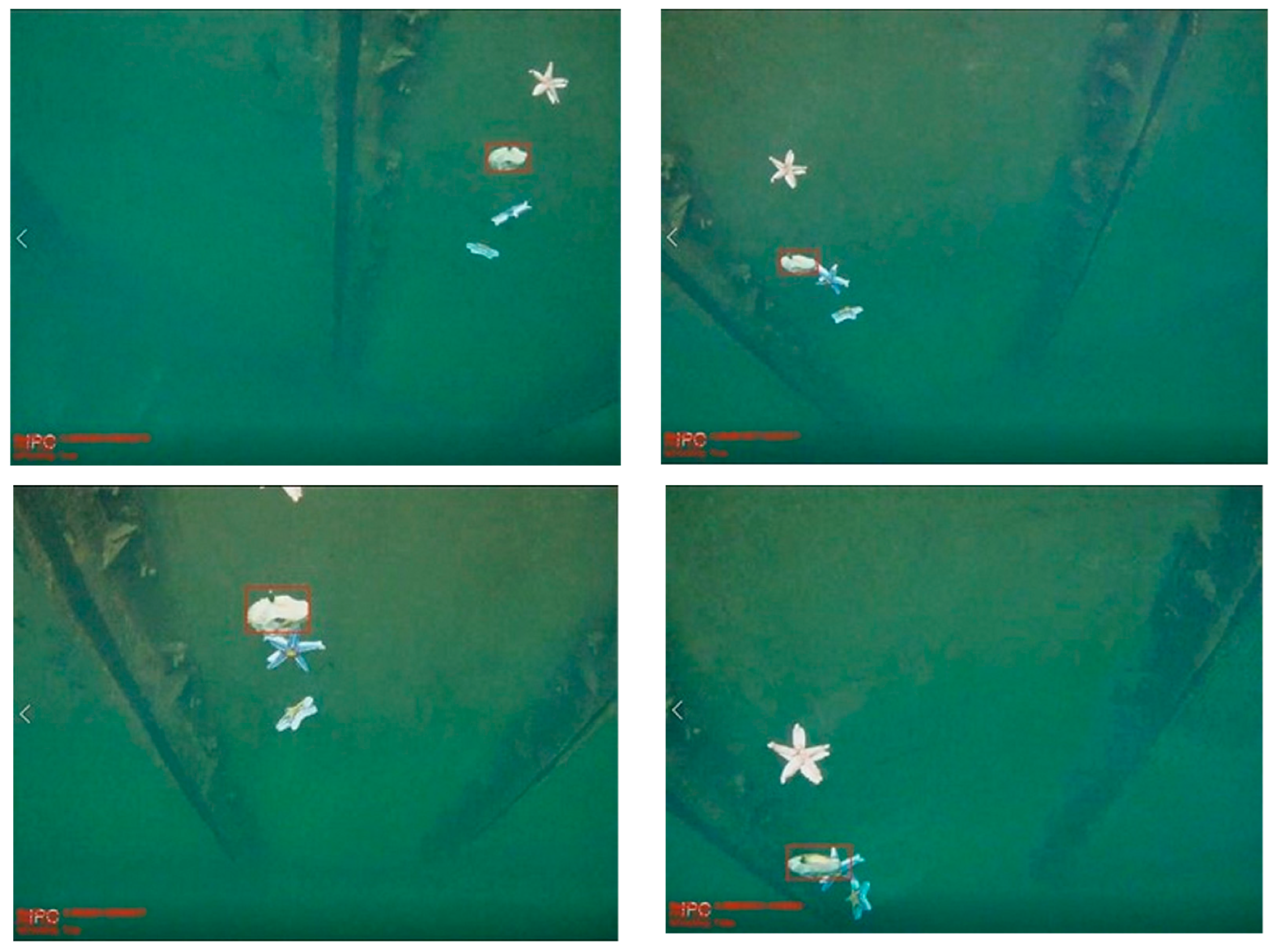
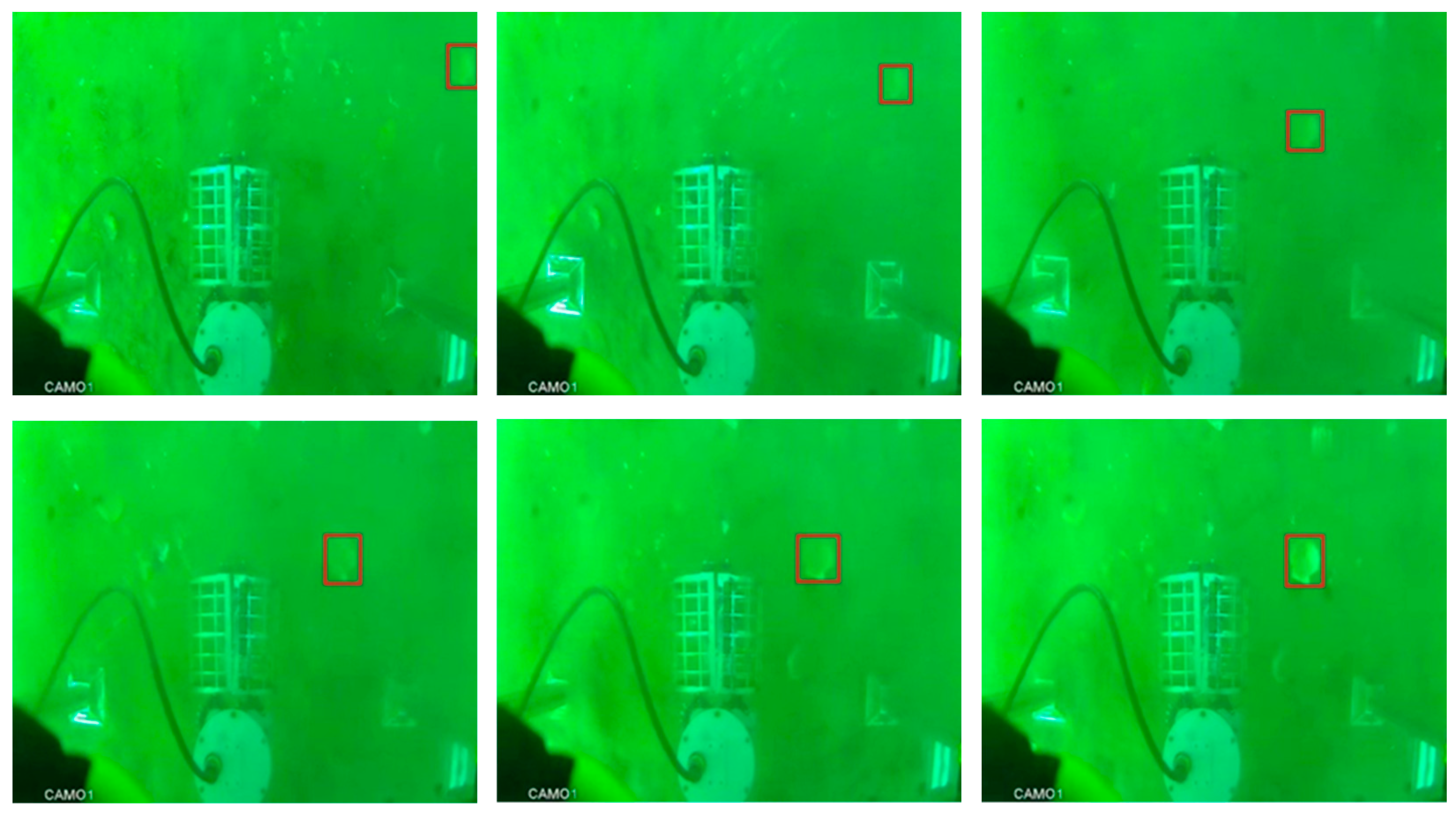
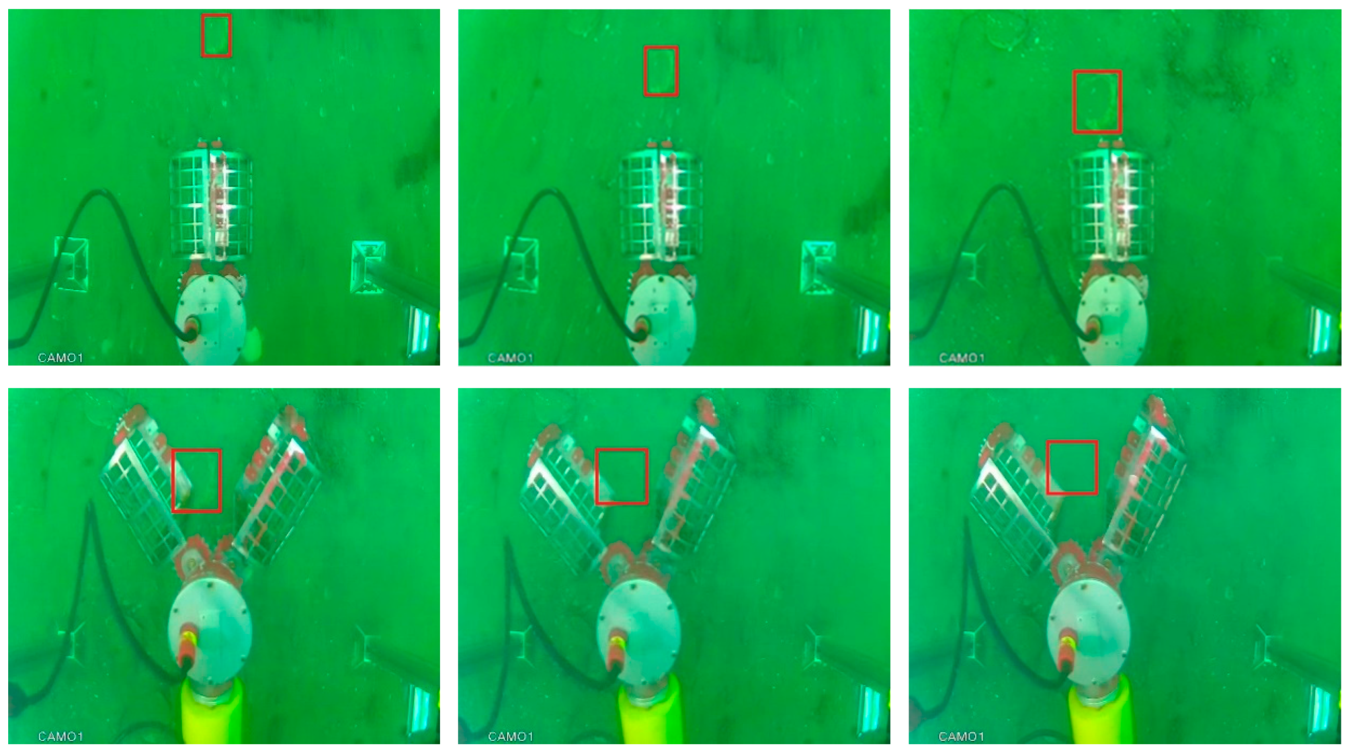
Firstly, the underwater dataset was used to validate the proposed algorithm. The advancement of the proposed algorithm can be seen qualitatively from the pictures presented in this paper. Figure 13, Figure 14, Figure 15 and Figure 16 show some underwater tracking effects. The red boxes in the figures represent the tracking box. The lower left corner shows the score, frame rate, and whether to track the target. Figure 13 shows the tracking effect when the target is a sea urchin. It can be seen that the tracking will not be disturbed by nontargets such as starfish and lobster in the field of view. Figure 14 and Figure 15 show the tracking effect when the target is a starfish. Compared with Figure 14, the background environment is more complex and has a good tracking effect at all positions of the field of view. Given the similar interference, scale change, target occlusion, and disappearance reproduction, the algorithm in this paper can still produce good tracking results. For example, the last picture in Figure 14 is the real-time tracking effect of the starfish target disappearing from the field of view and returning to the field of view. It can be seen that the tracking response is rapid, and the regression effect of the box is very good. As can be seen from the fourth picture in Figure 15, there is interference similar to the appearance of the target starfish, and part of the target starfish structure is obscured. This algorithm can clearly distinguish the tracking target without interference. It can be seen from the last two pictures in Figure 15 that when the starfish has a large shape change (such as the change from front to side caused by camera movement or angle change), the target can still be tracked and the size of the tracking frame can be adjusted with the shape change. Figure 16 shows the tracking effect of scallops at different positions and angles in the field of vision. Figure 17 shows the tracking results of sea cucumber targets, with relatively different backgrounds, reflecting the ability of the algorithm to deal with complex and diverse underwater environments. Figure 17 and Figure 18 show the tracking effect under the influence of currents in a real undersea environment. It can be seen that the underwater target can still be tracked when it is affected by the visual effect brought by the currents, which can support the subsequent operation tasks.

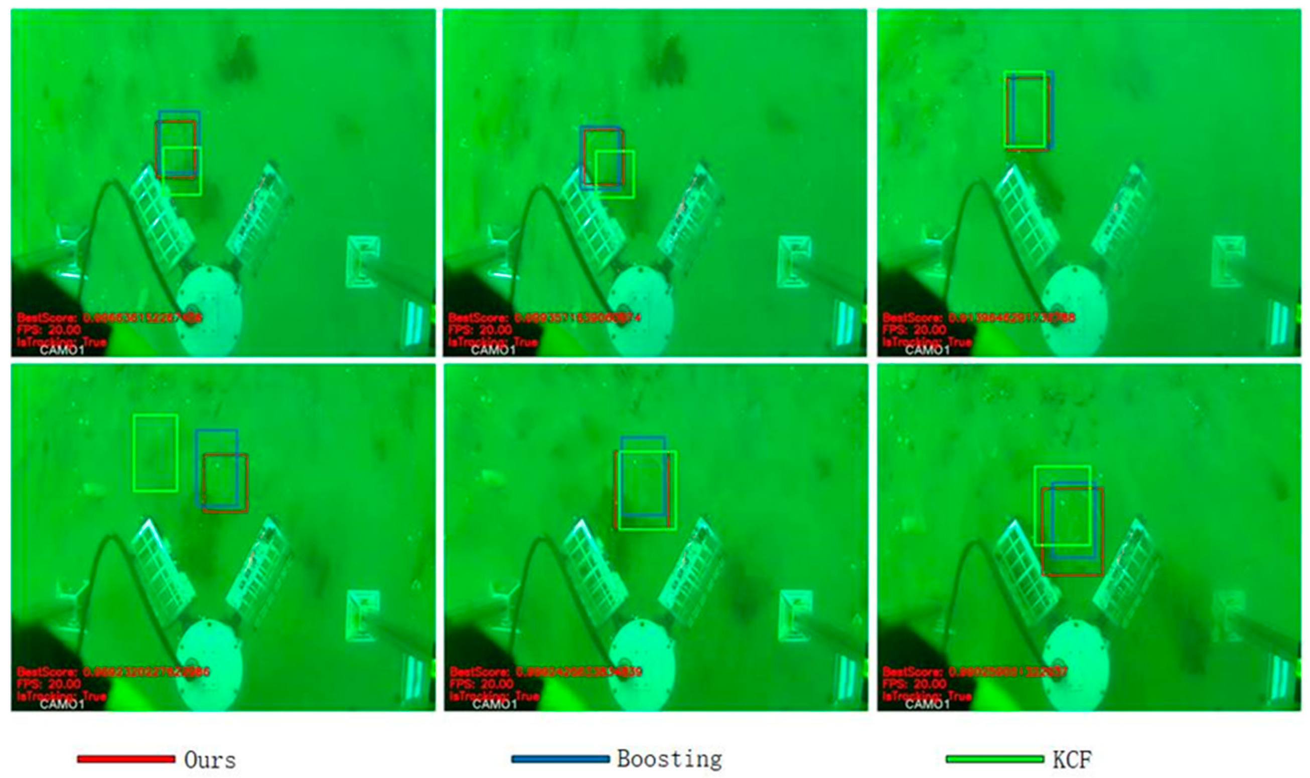
Compared to the Boosting and KCF algorithms, which are also widely used in underwater applications, the success rate comparison is shown in

Table 3. Comparison of the amount of computation and parameters of the network.

Tracker Name	Success Rate
Boosting	70.7%
KCF	65.9%
Ours	75.8%

. Compared to the correlation filter-based tracking algorithms Boosting and KCF, it is evident that the proposed algorithm is effective for underwater tracking tasks. Figure 19 shows the visual results of the three algorithms. The red rectangle indicates the algorithm proposed in this chapter, the blue rectangle represents the Boosting algorithm, and the green rectangle indicates the KCF algorithm. From Figure 1, it can be observed that the proposed algorithm can successfully track the target and has good box regression performance, while the other two methods exhibit varying degrees of tracking drift.

To evaluate the algorithm’s performance more comprehensively, comparisons were made with other deep learning methods on the OTB100 dataset. Figure 20a,b respectively show the success and precision curves of the proposed algorithm compared to other deep learning algorithms on the OTB100 dataset.

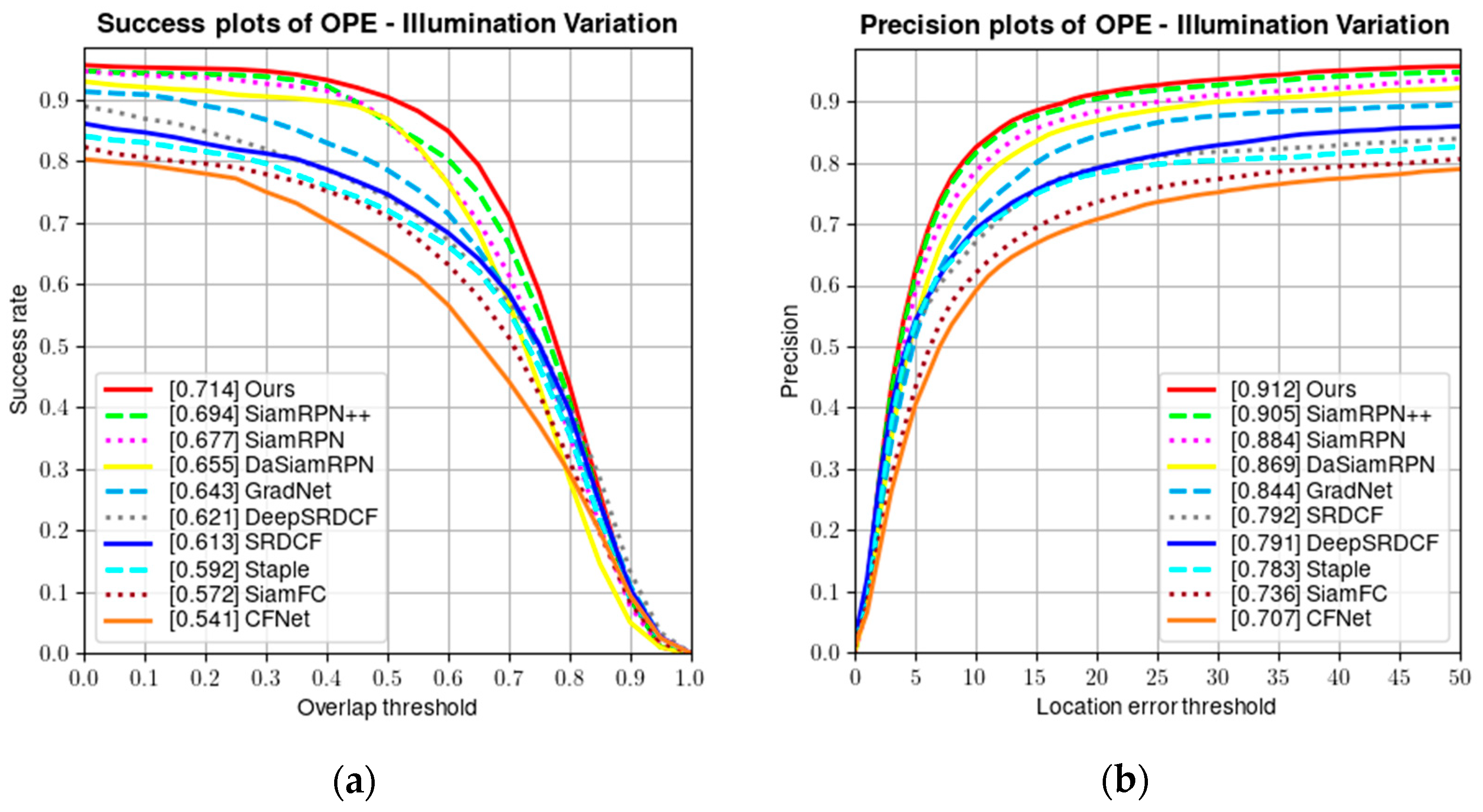
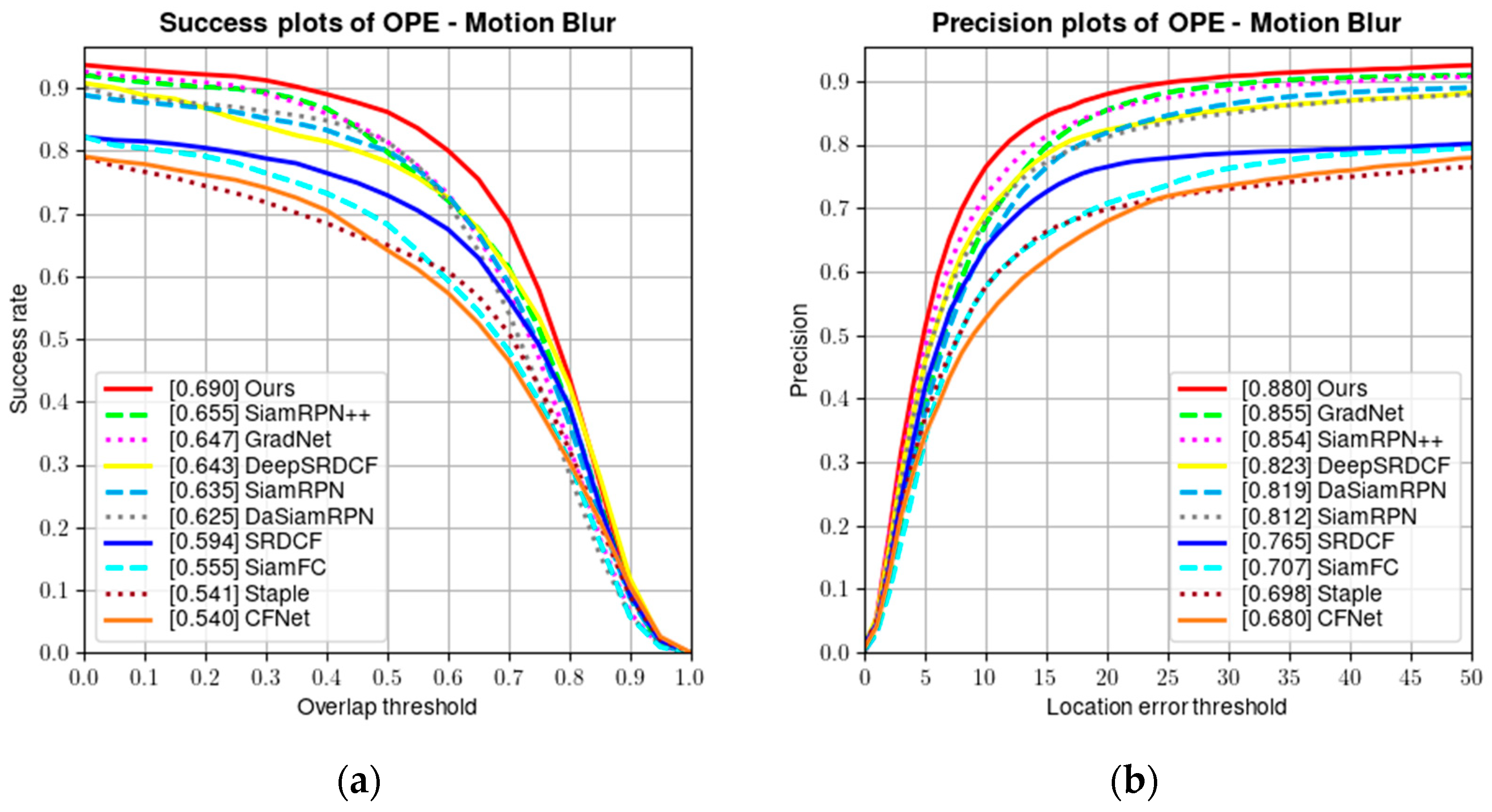
We also evaluated the performance of the algorithm using various factors present in the dataset. Figure 21a,b respectively show the success rate and accuracy of the algorithm after being interfered by illumination changes. Figure 22a,b respectively show the success rate and accuracy of the algorithm after being interfered by optical motion blur. Despite the interference from factors such as illumination variations and motion blur, the algorithm maintained a high level of success rate and precision.

To further demonstrate the superiority of the proposed algorithm, comparative experiments were conducted on the VOT2016 dataset with commonly used deep learning-based object tracking algorithms, including SiamRPN++ [8], DeepCSRDCF [12], CFCF [30], DSiam [9], SiamFC [26], and Staple [14]. The experimental results are shown in

Table 4. Test results on the VOT2016 dataset.

Tracker Name	Accuracy	Robustness	Lost Number	EAO
Ours	0.600	0.246	52.0	0.385
SiamRPN++	0.597	0.272	58.0	0.372
DeepCSRDCF	0.489	0.276	59.0	0.293
CFCF	0.511	0.286	61.0	0.280
DSiam	0.513	0.654	138.0	0.196
SiamFC	0.503	0.585	125.0	0.187
Staple	0.530	0.688	147.0	0.169

. The evaluation metrics used were accuracy, robustness, total loss, and expected average overlap. It can be observed that the proposed algorithm has certain advantages in all evaluation metrics.

6. Conclusions

This paper presents an object tracking algorithm for underwater vehicles based on the Siamese network and residual network, which combines the lightweight neural network model with the global feature model. The global feature model HE-Module is used to obtain the feature relationship between channels and spaces and to learn the motion excitation of the previous frame to obtain deeper foreground appearance features and semantic background, which enhances the computational performance and tracking accuracy of the algorithm. The lightweight neural network module is embedded in the residual network, which reduces the parameters of the model and facilitates the application of the algorithm to the work of the underwater vehicle. The evaluation is carried out on the collected underwater dataset, and the results show that the algorithm has good performance, including scale change, similar interference, and object occlusion. It has a good tracking effect in scale change, similar interference, object occlusion, and other situations.

Due to the lack of unified evaluation tools and standards for underwater tracking, we only calculated the intersection over the union between the tracking results and ground truth on our own collected underwater dataset. Using this evaluation method alone cannot fully reflect the performance of comprehensive tracking algorithms. Moreover, we used publicly available evaluation tools for non-underwater target tracking datasets. To address this issue, we need to collect and annotate underwater datasets and develop evaluation tools specifically for underwater tracking to establish a unified evaluation system in the field of underwater tracking.

References

1. Sun, Y.; Shi, Y.; Yun, X.; Wang, S. Adaptive strategy fusion target tracking based on multi-layer convolutional features. J. Electron. Inf. Technol. 2019, 41, 2464–2470. [Google Scholar] [CrossRef]
2. Yang, Z.; Li, Y.; Wang, B.; Ding, S.; Jiang, P. A lightweight sea surface object detection network for unmanned surface vehicles. J. Mar. Sci. Eng. 2022, 10, 965. [Google Scholar] [CrossRef]
3. Park, H.; Ham, S.-H.; Kim, T.; An, D. Object Recognition and Tracking in Moving Videos for Maritime Autonomous Surface Ships. J. Mar. Sci. Eng. 2022, 10, 841. [Google Scholar] [CrossRef]
4. Wu, Y.; Lim, J.; Yang, M.H. Online object tracking: A benchmark. In Proceedings of the IEEE Conference on Computer Vision and Pattern Recognition, Portland, OR, USA, 23–28 June 2013; pp. 2411–2418. [Google Scholar] [CrossRef]
5. Li, P.; Wang, D.; Wang, L.; Lu, H. Deep visual tracking: Review and experimental comparison. Pattern Recognit. 2018, 76, 323–338. [Google Scholar] [CrossRef]
6. Zuo, W.; Wu, X.; Lin, L.; Zhang, L.; Yang, M.-H. Learning support correlation filters for visual tracking. IEEE Trans. Pattern Anal. Mach. Intell. 2018, 41, 1158–1172. [Google Scholar] [CrossRef] [PubMed]
7. Freund, Y.; Schapire, R.E. A decision-theoretic generalization of on-line learning and an application to boosting. J. Comput. Syst. Sci. 1997, 55, 119–139. [Google Scholar] [CrossRef]
8. Li, B.; Wu, W.; Wang, Q.; Zhang, F.; Xing, J.; Yan, J. Siamrpn++: Evolution of siamese visual tracking with very deep networks. In Proceedings of the IEEE/CVF Conference on Computer Vision and Pattern Recognition, Long Beach, CA, USA, 15–20 June 2019; pp. 4282–4291. [Google Scholar] [CrossRef]
9. Zhu, Z.; Wang, Q.; Li, B.; Wu, W.; Yan, J.; Hu, W. Distractor-aware siamese networks for visual object tracking. In Proceedings of the European Conference on Computer Vision (ECCV), Munich, Germany, 8–14 September 2018; pp. 101–117. [Google Scholar] [CrossRef]
10. Valmadre, J.; Bertinetto, L.; Henriques, J.; Vedaldi, A.; Torr, P.H.S. End-to-end representation learning for correlation filter based tracking. In Proceedings of the IEEE Conference on Computer Vision and Pattern Recognition, Honolulu, HI, USA, 21–26 July 2017; pp. 2805–2813. [Google Scholar] [CrossRef]
11. Li, P.; Chen, B.; Ouyang, W.; Wang, D.; Yang, X.; Lu, H. Gradnet: Gradient-guided network for visual object tracking. In Proceedings of the IEEE/CVF International Conference on Computer Vision, Seoul, Republic of Korea, 27 October–2 November 2019; pp. 6162–6171. [Google Scholar] [CrossRef]
12. Danelljan, M.; Hager, G.; Shahbaz Khan, F.; Felsberg, M. Convolutional features for correlation filter based visual tracking. In Proceedings of the IEEE International Conference on Computer Vision Workshops, Santiago, Chile, 7–13 December 2015; pp. 58–66. [Google Scholar] [CrossRef]
13. Li, F.; Tian, C.; Zuo, W.; Zhang, L.; Yang, M.H. Learning spatial-temporal regularized correlation filters for visual tracking. In Proceedings of the IEEE Conference on Computer Vision and Pattern Recognition, Salt Lake City, UT, USA, 18–23 June 2018; pp. 4904–4913. [Google Scholar] [CrossRef]
14. Bertinetto, L.; Valmadre, J.; Golodetz, S.; Miksik, O.; Torr, P.H.S. Staple: Complementary learners for real-time tracking. In Proceedings of the IEEE Conference on Computer Vision and Pattern Recognition, Las Vegas, NV, USA, 26 June–1 July 2016; pp. 1401–1409. [Google Scholar] [CrossRef]
15. Cui, Y.; Jiang, C.; Wang, L.; Wu, G. Mixformer: End-to-end tracking with iterative mixed attention. In Proceedings of the IEEE/CVF Conference on Computer Vision and Pattern Recognition, New Orleans, LA, USA, 18–24 June 2022; pp. 13608–13618. [Google Scholar] [CrossRef]
16. Ye, B.; Chang, H.; Ma, B.; Shan, S.; Chen, X. Joint feature learning and relation modeling for tracking: A one-stream framework. In Proceedings of the Computer Vision–ECCV 2022: 17th European Conference, Tel Aviv, Israel, 23–27 October 2022; pp. 341–357. [Google Scholar] [CrossRef]
17. Ortiz, A.; Simó, M.; Oliver, G. A vision system for an underwater cable tracker. Mach. Vis. Appl. 2002, 13, 129–140. [Google Scholar] [CrossRef]
18. He, K.; Zhang, X.; Ren, S.; Sun, J. Deep residual learning for image recognition. In Proceedings of the IEEE Conference on Computer Vision and Pattern Recognition, Las Vegas, NV, USA, 26 June–1 July 2016; pp. 770–778. [Google Scholar] [CrossRef]
19. Li, A.; Yu, L.; Tian, S. Underwater Biological Detection Based on YOLOv4 Combined with Channel Attention. J. Mar. Sci. Eng. 2022, 10, 469. [Google Scholar] [CrossRef]
20. Hong, X.; Cui, B.; Chen, W.; Rao, Y.; Chen, Y. Research on Multi-Ship Target Detection and Tracking Method Based on Camera in Complex Scenes. J. Mar. Sci. Eng. 2022, 10, 978. [Google Scholar] [CrossRef]
21. Kong, Z.; Cui, Y.; Xiong, W.; Yang, F.; Xiong, Z.; Xu, P. Ship target identification via Bayesian-transformer neural network. J. Mar. Sci. Eng. 2022, 10, 577. [Google Scholar] [CrossRef]
22. Li, B.; Yan, J.; Wu, W.; Zhu, Z.; Hu, X. High performance visual tracking with siamese region proposal network. In Proceedings of the IEEE Conference on Computer Vision and Pattern Recognition, Salt Lake City, UT, USA, 18–23 June 2018; pp. 8971–8980. [Google Scholar] [CrossRef]
23. Girshick, R. Fast r-cnn. In Proceedings of the IEEE International Conference on Computer Vision, Santiago, Chile, 7–13 December 2015; pp. 1440–1448. [Google Scholar] [CrossRef]
24. Lin, T.Y.; Dollár, P.; Girshick, R.; He, K.; Hariharan, B.; Belongie, S. Feature pyramid networks for object detection. In Proceedings of the IEEE Conference on Computer Vision and Pattern Recognition, Honolulu, HI, USA, 21–26 July 2017; pp. 2117–2125. [Google Scholar] [CrossRef]
25. Hu, J.; Shen, L.; Sun, G. Squeeze-and-excitation networks. In Proceedings of the IEEE Conference on Computer Vision and Pattern Recognition, Salt Lake City, UT, USA, 18–23 June 2018; pp. 7132–7141. [Google Scholar] [CrossRef]
26. Bertinetto, L.; Valmadre, J.; Henriques, J.F.; Vedaldi, A.; Torr, P.H. Fully-convolutional siamese networks for object tracking. In Computer Vision–ECCV 2016 Workshops: Amsterdam, The Netherlands, October 8–10 and 15–16, 2016, Proceedings, Part II 14; Springer International Publishing: Berlin/Heidelberg, Germany, 2016; pp. 850–865. [Google Scholar] [CrossRef]
27. Russakovsky, O.; Deng, J.; Su, H.; Krause, J.; Satheesh, S.; Ma, S.; Huang, Z.; Karpathy, A.; Khosla, A.; Bernstein, M.; et al. Imagenet large scale visual recognition challenge. Int. J. Comput. Vis. 2015, 115, 211–252. [Google Scholar] [CrossRef]
28. Wu, Y.; Lim, J.; Yang, M.H. Object tracking benchmark. IEEE Trans. Pattern Anal. Mach. Intell. 2015, 37, 1834–1848. [Google Scholar] [CrossRef] [PubMed]
29. Čehovin, L.; Leonardis, A.; Kristan, M. Visual object tracking performance measures revisited. IEEE Trans. Image Process. 2016, 25, 1261–1274. [Google Scholar] [CrossRef] [PubMed]
30. Gundogdu, E.; Alatan, A.A. Good features to correlate for visual tracking. IEEE Trans. Image Process. 2018, 27, 2526–2540. [Google Scholar] [CrossRef] [PubMed]
Figure 1. Architecture for the autonomous control and target tracking of underwater vehicles.
Jmse 11 01127 g001
Figure 2. The structure of SiamRPN.
Jmse 11 01127 g002
Figure 3. The structure of lightweight neural network model.
Jmse 11 01127 g003
Figure 4. The structure of spatial excitation.
Jmse 11 01127 g004
Figure 5. The structure of channel excitation.
Jmse 11 01127 g005
Figure 6. The structure of motion excitation method.
Jmse 11 01127 g006
Figure 7. The structure of HE-Module.
Jmse 11 01127 g007
Figure 8. The structure of the residual block.
Jmse 11 01127 g008
Figure 9. Siamese network framework.
Jmse 11 01127 g009
Figure 10. The structure of SL-HENet.
Jmse 11 01127 g010
Figure 11. Tracking strategy diagram.
Jmse 11 01127 g011
Figure 12. Depth variation of the underwater vehicle.
Jmse 11 01127 g012
Figure 13. Tracking results of sea urchins in underwater video.
Jmse 11 01127 g013
Figure 14. Tracking results of starfish with scale change in underwater video.
Jmse 11 01127 g014
Figure 15. Tracking results of starfish with scale change in underwater video.
Jmse 11 01127 g015
Figure 16. Tracking results of scallops in underwater video.
Jmse 11 01127 g016
Figure 17. Tracking results under the influence of currents.
Jmse 11 01127 g017
Figure 18. Tracking results when visual effects are affected by currents.
Jmse 11 01127 g018
Figure 19. Underwater algorithm contrast visualization.
Jmse 11 01127 g019
Figure 20. Comparison of each algorithm on OTB100 dataset; (a) success rate curves; (b) precision curves.
Jmse 11 01127 g020
Figure 21. Comparison of algorithms under the interference of illumination variation; (a) success rate curves; (b) precision curves.
Jmse 11 01127 g021
Figure 22. Comparison of algorithms under the interference of motion blur; (a) success rate curves; (b) precision curves.
Jmse 11 01127 g022