1. Introduction
Flooding incidents of damaged ships have received increasing attention in recent decades. Various flooding accidents have prompted researchers to study them. Therefore, the importance of the ability to make decisions rapidly during floods has also been emphasized by researchers. Hasty evacuation procedures will increase the risk of crews in ship during the flooding [
1]. In various types of ships, when flooding accidents occur on large passenger ships, the decision to evacuate becomes particularly difficult because of the size of the crew. So, if large passenger ships are damaged, decision-makers require more flooding information to make decisions. During a flooding event, having thousands of crewmembers makes evacuation procedures time-consuming. In order to reduce the flood-related casualties and economic losses, decision-makers must make evacuation decisions as quickly as possible when the passenger ship is damaged and deemed no longer safe or will capsize.
Most ships are designed with watertight equipment to deal with sudden flooding events. In addition to this, many options have been used to evaluate risk after a ship is damaged [
2]. Some passenger ships are equipped with computers that can assess damage stability. However, these stability computers are driven with algorithms and mechanical formulas embedded in advance. Not only do the parameters of the compartment need to be entered manually, but the impact of flooding on the ship is also difficult to assess [
3]. This could cause a ship to capsize before it reaches the final balance state of flooding. Decisions then become meaningless. Hereafter, researchers develop various progressive flooding simulation codes and apply them to ships [
4,
5]. These codes are combined with real-time visualization techniques and graphical user interfaces to form a complete decision support system. A new flooding simulation method has been developed by Dankowski [
6]. The method can capture the progression flooding process. This method provides a fast and straightforward tool for the research of the flooding process in the time domain. Pekka proposed a simplified method for quickly predicting flooding information on damaged ships, based on level sensors [
7]. This method obtains satisfactory results during flooding progression. Based on the condition of level sensors, a novel method has been presented for breach assessment on damaged ships [
8]. The method can be used for progressive flooding prediction if a ship is equipped with a sufficient number level sensor. Different theories have been proposed to simplify the flooding process and improve computational efficiency [
9,
10,
11]. Even so, such a decision support system is time-consuming when it makes decisions. As well, strong and powerful hardware support is a must, for example, servers supporting distributed computing technology [
12].
The earliest research on ship flooding focused on experiments with model ships. Among them, the International Towing Tank Conference (ITTC) organized a benchmark study on ship flooding earlier. van Walree and Papanikolaou [
13] focused on model tests using box-shaped barges and used experimental data to drive the development of progressive flooding theory. These physical experiment methods come at a huge cost [
14,
15]. It is often carried out to verify the theory proposed by researchers and to study some specific phenomena [
16,
17].
Progressive flooding code and CFD toolkit are mainstream methods of ship flooding research. Different countries and regions have some similar research methods. These codes often calculate the flooding rate based on the Bernoulli equation, and the discharge coefficient is a constant or selected empirical value. This method cooperates with the stability computer and other hardware on large passenger ships to form various decision-making systems on board. In addition, the researchers also used these codes to trace back flooding accidents, capture the hydrodynamic phenomena during flooding, predict the flooding time of the compartment, etc. Progressive flooding codes are generally owned internally by research institutions and are called in-house codes, such as PROTEUS, originally developed by the University of Strathclyde (MSRC) and owned by Brooks Bell (BROO) subsidiary Safety at Sea Ltd. (Glasgow, UK). In this code, the flooding rate is determined by the Bernoulli equation, the discharge coefficient is constant at 0.6, and the flooding motion is modeled as a pendulum. Ship motion has six degrees of freedom. Details are presented in Jasionowski [
18]. SMTP is the in-house code of the Korea Research Institute of Ships and Ocean Engineering. The flooding rate is also calculated by the Bernoulli equation. This code uses empirical discharge coefficients and offers many types of compartments and openings. Ship motions are computed by six degrees of freedom nonlinear equations in the time domain. Details are presented in Lee [
19].
Some codes are combined with the computing power of high-performance computers. This is the CFD toolkit. According to different flooding scenarios, there is a more detailed theoretical division (Reynolds-averaged Navier–Stokes, Unsteady Reynolds-averaged Navier–Stokes, quasi-static theory). For example, the commercial CFD software Star-CCM+ uses the Volume of Fluid (VOF) method for flooding. Both regular and irregular waves can be invoked in the simulation. Details of the method are in Bu and Gu [
20,
21]. The Open FOAM CFD Toolbox is where air cand water flows are solved through finite volume formulations, solving the Reynolds-averaged Navier–Stokes equations. For details on using CFD in flood analysis, see Ruth et al. [
22]. Similar CFD software packages for ship flooding time calculation include NAPA (quasi-static method), ComFLOW.
The CFD methods can accurately predict the ship’s motion after it is damaged [
23,
24]. The hydrodynamic phenomenon in the compartment can also be completely captured [
25,
26]. However, the price of the good prediction effect of CFD methods is long iterative calculations [
27]. Sometimes fine meshing is also required (e.g., overlapping meshes) [
28]. Obviously, neither two methods are better for sudden emergencies.
In the past five years, machine learning techniques have been combined with ship flooding. Luca Braidotti simplified the emergency decision support system on ship, and a flooding sensor-independent method was proposed [
29]. A progressive flood simulation was employed using a database-trained machine learning algorithm to assess the main consequences of a damage scenario. Furthermore, the application of random forests was proved to be suitable for assessing the final state of ships and damaged compartment settings and estimating flooding time [
30].
In fact, the process of flooding spreading in the compartment at an early stage will imply information on how flooding will evolve in the future. Simply put, when the flooding water is rapid, the time for the compartment to be filled will be shorter. Normally, monitoring equipment will be installed in an important position (engine room) on large passenger ships to observe the compartments. It means that when the compartments are flooded, camera equipment can record the video of the flooding in real-time. When these videos are processed into images, the information contained in the flooding water changes is also fixed. This makes it possible to obtain flooding information through convolutional neural networks. Since the convolutional neural network came out [
31], its powerful ability to acquire spatial information has been verified. In the last few years, convolutional neural networks have developed different frameworks. The residual neural network [
32] is the most representative. At present, many residual networks with different structures have been presented [
33,
34,
35,
36]. Additionally, recurrent neural networks perform well for modeling time series. There have been many achievements in machine translation [
37,
38], sentiment analysis [
39,
40], stock prediction [
41], and other fields. Significant temporal correlation of ship flooding fits with recurrent neural networks.
The European Union’s Horizon 2020 project, FLARE, organized a new benchmarking study. The first part of the study focuses on flooding mechanisms in different flooding scenarios. One of the sub-projects is the large horizontal flooding of an area with a typical deck layout in a cruise ship. The research mainly measured and recorded the water level in the flooded compartment. Several of the progressive flooding codes and CFD software were involved as research tools. Because of the current international emphasis on the research on the flooding of cruise compartments, especially the measured and recorded water level and flooding time of compartments in calm water. This paper proposes a new method to obtain these focused data, using the method of deep learning to achieve this task.
In the early stage of flooding, the flooding water’s movement on board implies information on how flooding water will change in the future. Based on these, this paper explores the feasibility of predicting the flooding time of the compartment based on the flooding image. To this end, a composite neural network is adopted, that is, a CNN–RNN framework. The neural network proposed in this paper is trained and tested using datasets obtained from physical experiments.
The first part describes some methods of researching ship flooding and illustrates the related works. The next part describes the combining of flooding images and neural networks and introduces the neural network architecture in the paper. The fourth part introduces the flooding experiment and the datasets, and the fifth part is the experiment and discussion, and the final part is the conclusion.
2. Methodology
When the integrity of the hull cannot be guaranteed due to damage (collision, grounding, etc.), this is the beginning of a flooding event. Flooding water will enter damaged compartments through openings and spread across through non-watertight doors (e.g., fire doors, light connector doors, etc.). The movement of water obeys a host of the laws of physics. Therefore, information on flooding water is predictable. If the time cost is not considered too much, the progressive flooding simulation code can accomplish this task very well. However, when a flooding accident occurs, a shorter decision-making time is better. Among the decisions required, the flooding time of the compartment is the key information needed for decision-making. It determines the shortest evacuation time for crews in flooded compartments. It is also important information that decision-makers should provide to crews after flooding. The flooding images are key information for flooding time perdition. Next, we will illustrate how to use the flooding images in a neural network.
2.1. Process Sketch
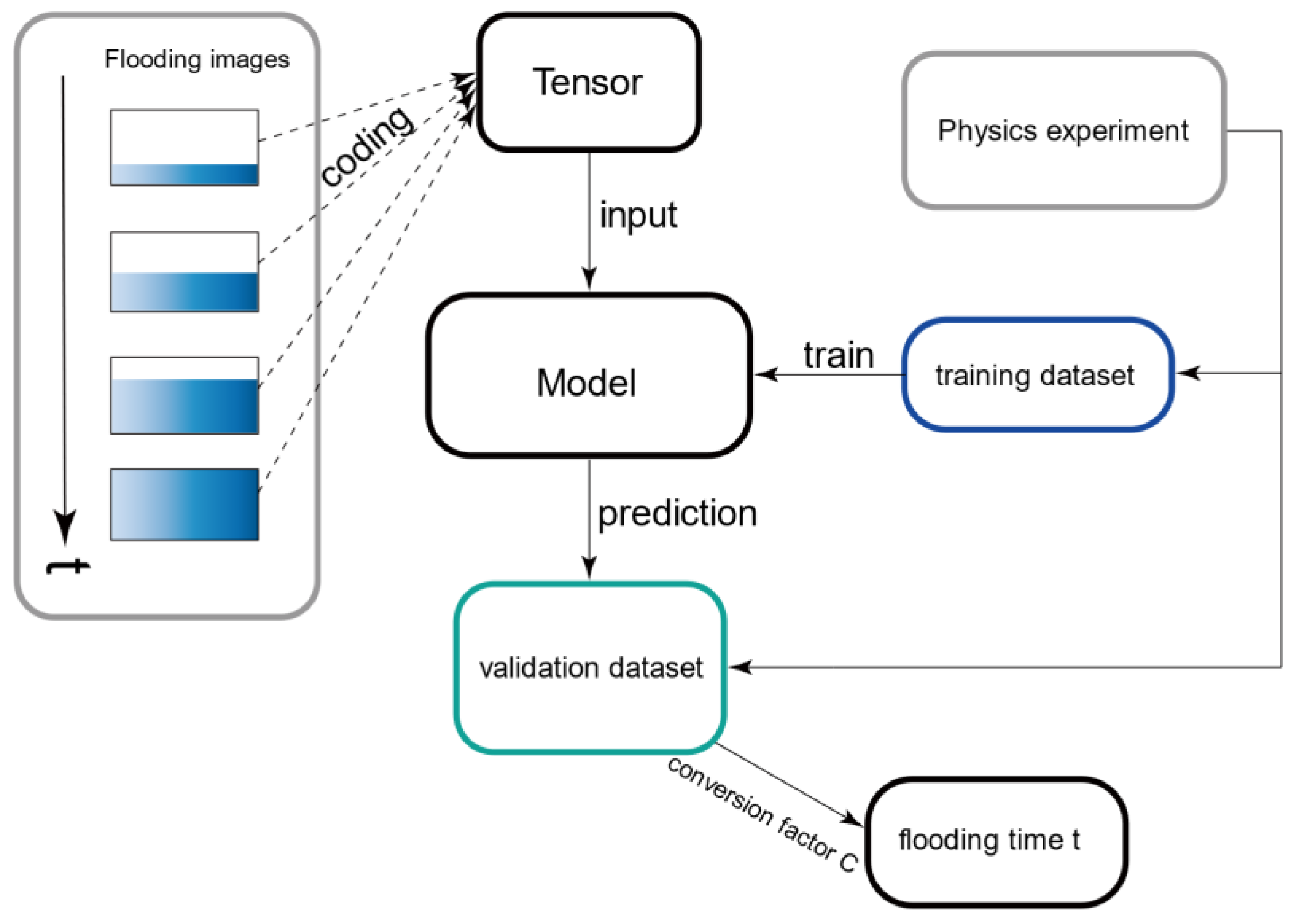
In this paper, the flooding images of the damaged compartment are used to predict the time for the flooding water to reach the specified height (referred to as the flooding time, tf). In order to make this idea easy to realize, the selected flooding images have two characteristics: First, the flooding images are an ordered set that evolves over time. In practice, considering the limited working time of the recording equipment in the flooded compartments, the evolution time needs to be as short as possible. Only then the images required for prediction are obtained from the damaged compartment. This reduces the workload and makes flooding images easy to get, as well.
The process sketch of the complete flooding time prediction is shown in
Figure 1. In
Figure 1, the input of the composite neural network is the flooding images provided by the physical experiment. The final output of the composite neural network is the
tf of the target compartments.
2.2. Conversion of Flooding Time for Cruise Ship and Model Ship
The physical experiment is carried out using the cruise model with a scale ratio of 200. The composite neural network is trained by the data obtained in the experiment. Because the flooding time obtained by the experiment is too small, the problem cannot be explained intuitively. Here it is necessary to transform the predicted results to the real ship(cruise) angle. Therefore, it is critical to determine the flooding time conversion coefficient C between the model and the real ship.
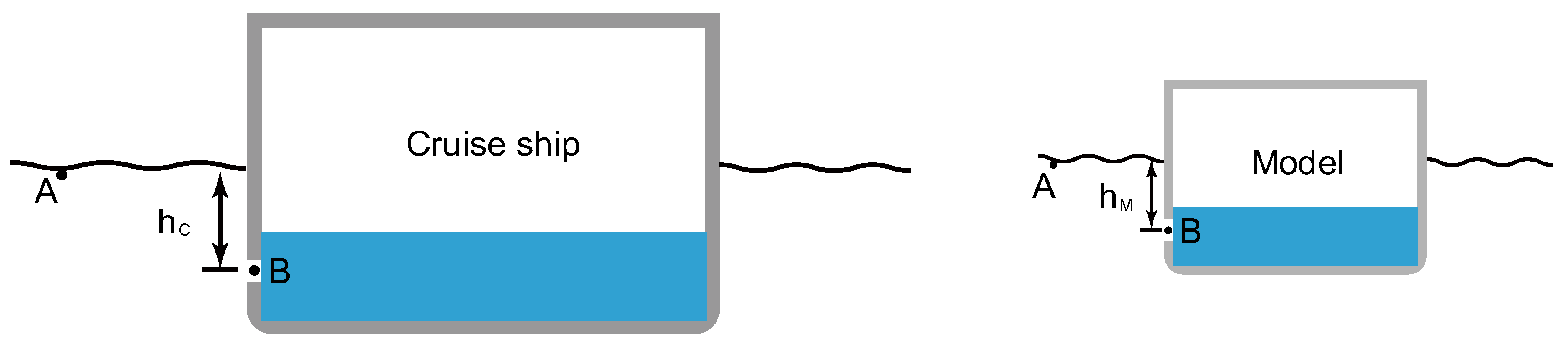
This problem can be solved through mathematical modeling. The first step is at the same location, determining the water velocity of the model and the cruise. The following scenarios can be set up for the same opening location as shown in
Figure 2.
According to Bernoulli’s principle, Equation (1) can be obtained:
where
PA, and
PB are the pressures at points
A and
B, respectively, and take the value of atmospheric pressure,
ρ is the density of water,
,
are the velocity of water at points
A and
B, respectively, and
is the acceleration of gravity.
,
are the depths from points
A and
B, respectively, to the grounding of the water.
is the pressure loss coefficient. Since the external environment is still water,
is 0. Arranging and obtaining the water velocity expression of point
B, we obtain Equation (2):
where
Cd is the flow coefficient of the opening, which is a constant. For the cruise ship,
is
in
Figure 2, and for the model, it is
. The relationship between the water speed of the cruise ship and the model at the same opening is shown in Equation (3):
where
is the scaling ratio; the value is 200.
The ratio of the cross-sectional area (
S) of the cruise ship to the model is
, and the ratio of the volume (
V) is
. Therefore, the conversion coefficient
C of the flooding time of the cruise ship and the model is obtained, as shown in Equation (4):
Hence, the flooding time of the model is 1 s and that of the cruise ship is about 14.14 s.
2.3. Framework
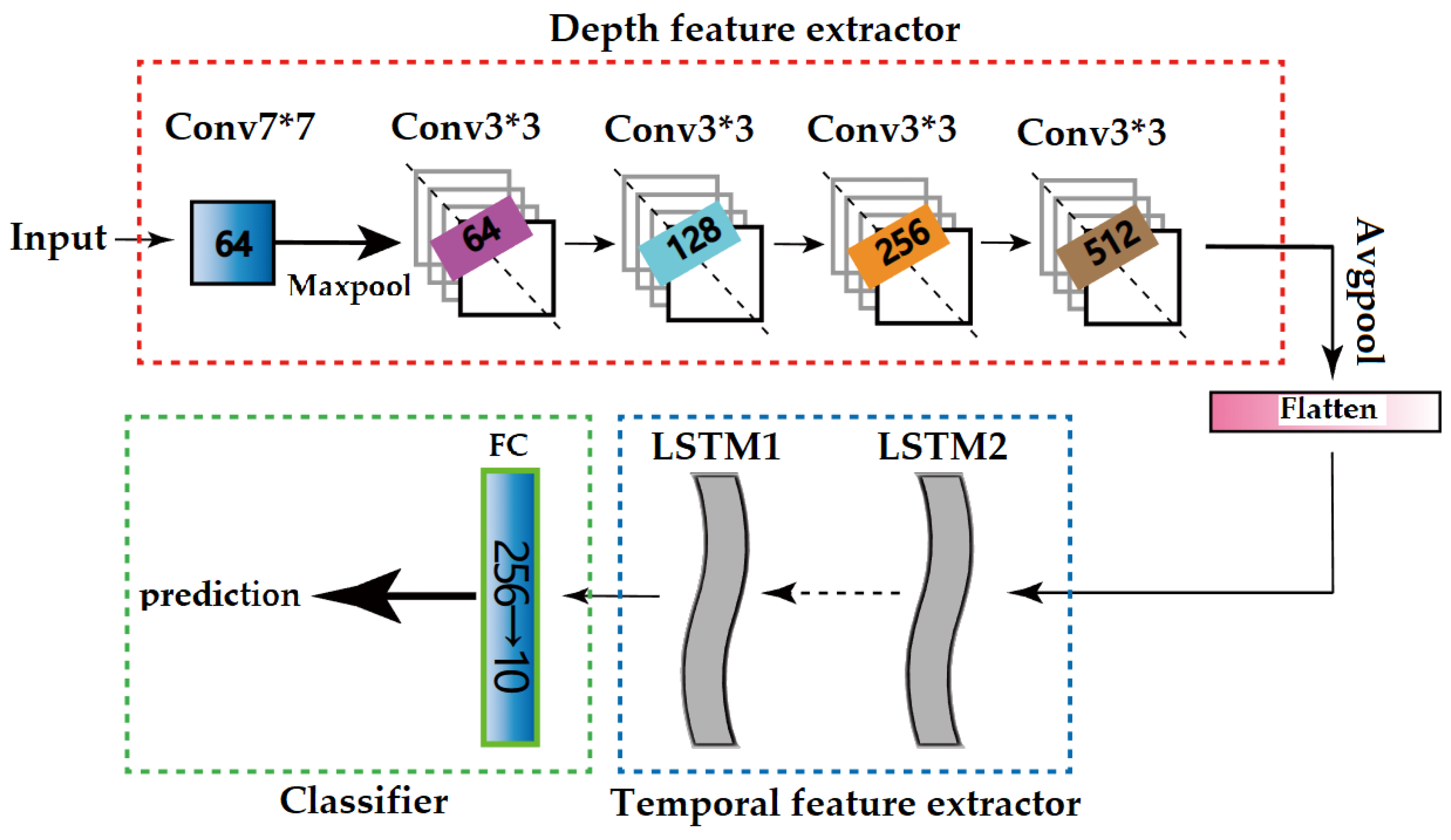
A composite neural network based on CNN–RNN is used in this paper. Flooding images are obtained from flooding video clips. The CNN part extracts the spatial information of images and outputs a tensor. Then, this tensor is input into the RNN part, and the temporal features are extracted in the RNN part. Its structure is shown in
Figure 3.
2.3.1. Depth Feature Extractor
Before training the model, the flooding video obtained in the experiment needs to be edited into images with a size of 1920 × 1440. One flooding video obtained a batch of flooding images. These images will be extracted into relevant features through 2D CNN. The input of the composite neural network is the batch of flooding images. We choose the ResNet18 architecture as the 2D CNN model. This is due to its proven accuracy and low computational cost [
42]. Using the idea of migration learning, the trained ResNet18 architecture is used in the pre-processing stage. This architecture is available in the Pytorch [
43] deep learning package.
Since the purpose of 2D CNN here is to extract features of flooding water rather than classification, we removed the last fully connected layer and SoftMax output layer of ResNet18. Before being input to the ResNet18 architecture, the flooding image will be redefined as a tensor of size 512 × 276 × 3 during pre-processing. Then, flooding images are put into the maximum pooling layer, five convolutional layers. One of the convolutional layers has a kernels size of seven and output channel of 64. The rest of the convolutional layer has a kernels size of three, and the output channels are 64, 128, 256, 512. The way of information flow is shown in
Figure 3. After depth feature extractor, it is flattened to 2048 × 1 by the flattened layer. If there are t-second sequences for training, the input size to the RNN is
t × 2048 × 1.
2.3.2. Temporal Feature Extract
Ship flooding is a continuous process. In order to quickly obtain prediction results, the timescales of flooding videos generally range from seconds to minutes. A Long Short-Term Memory network is chosen for this task. LSTM networks have advantages in longer time series training. It is less susceptible to the vanishing gradient problem than standard RNNs. This makes LSTM a suitable choice for temporal feature extract in our paper.
A general LSTM unit consists of an input gate
i, an output gate
o and a forget gate
f shown in Equation (5), where
ht − 1 is the hidden state at the
t − 1 s, and
xt is the input of the LSTM at the current moment.
Hidden state and cell state at the current moment is determined by Equations (6) and (7):
The weight matrix
W contains learnable parameters. The sigmoid function is given by Equation (8):
The LSTM architecture used here is many-to-many. Because there is a series of tensors fed into the LSTM network, and the outcome to predict is four. The neural network in this paper performs classification prediction. The result of the prediction is the label of the time interval. For a ship, the amount of data available is limited. After testing, if the regression prediction is performed, the neural network can easily fall into a local optimal solution. In fact, the effect of regression prediction can be approximated as much as possible by dividing the time interval. The hyperparameters of the RNN part are obtained by referring to the literature [
42] with similar tasks, as shown in
Table 1. The optimization method is Adaptive Moment Estimation (Adam) algorithm in Pytorch.
The loss function uses a composite form. The overall loss function consists of four parts, because all four compartments are involved in the prediction of the framework. Every part uses the cross-entropy function. This function is suitable for classification problems [
44,
45], and its function expression is shown in Equation (9):
Among them: p(x), q(x) represents the predicted and target value of flooding time, respectively. In this paper n takes the value of 10.
The neural network will give the predicted flooding times (
tf)
p1,
p2,
p3,
p4 for four compartments. These predicted values and target values
q1,
q2,
q3,
q4 are put into the cross-entropy function to obtain the loss values
L1,
L2,
L3,
L4. Then, all the loss values are summed to obtain the final loss value
LS. This loss value is the final value participating in the backpropagation, shown in Equation (10):
3. Flooding Experiment and Dataset
3.1. Parameters
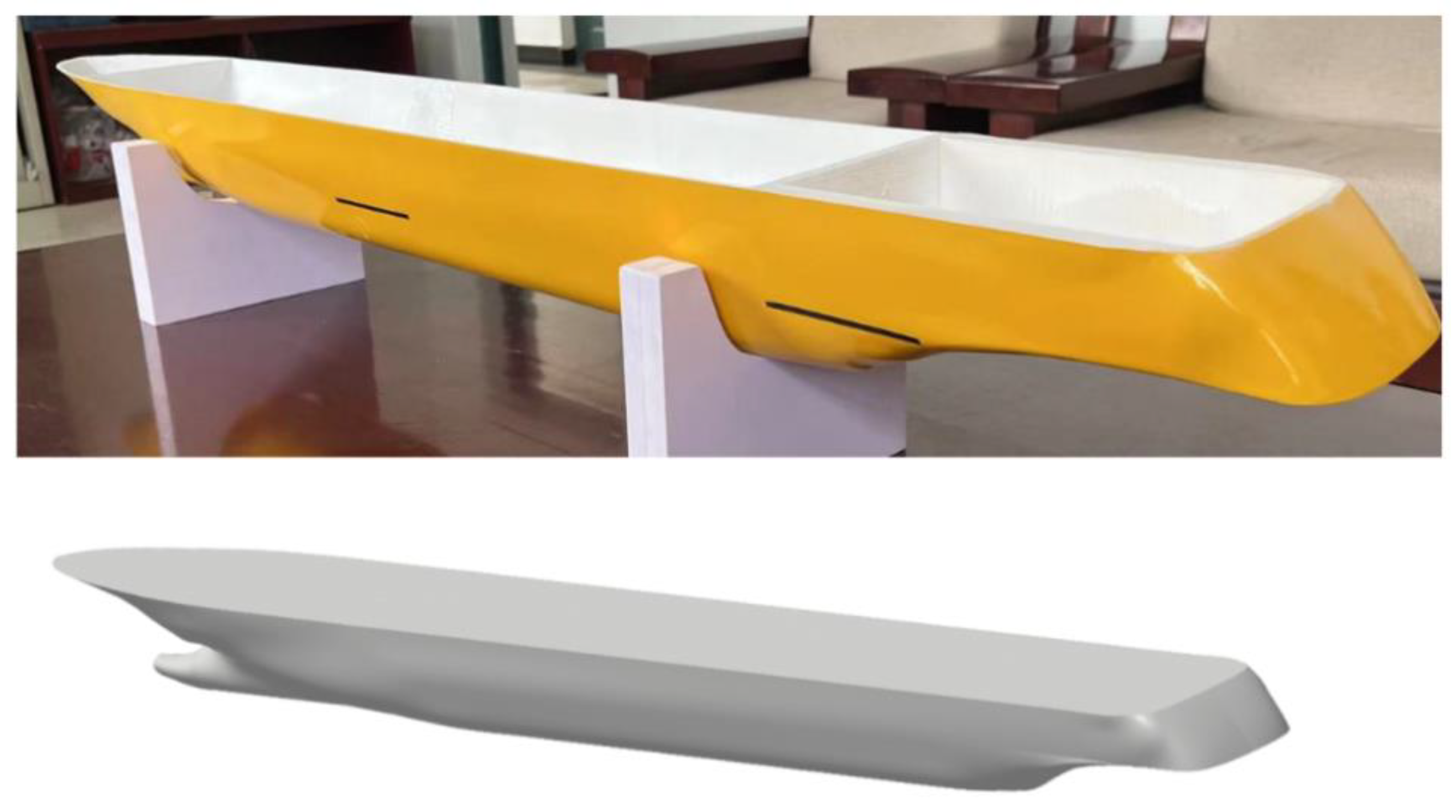
To obtain a dataset for training, a flooding experiment is implemented. The experimental object is a ship model. Its prototype is a cruise ship.
The model has a scale ratio of 1:200 and is made to use 3D printing technology. The portion below the main deck of the cruise ship is fabricated for the flooding experiment.
Table 2 shows the details of the model and cruise ship.
The 3D drawing of the model and the actual finished product are shown in
Figure 4:
3.2. Flooding Scenario
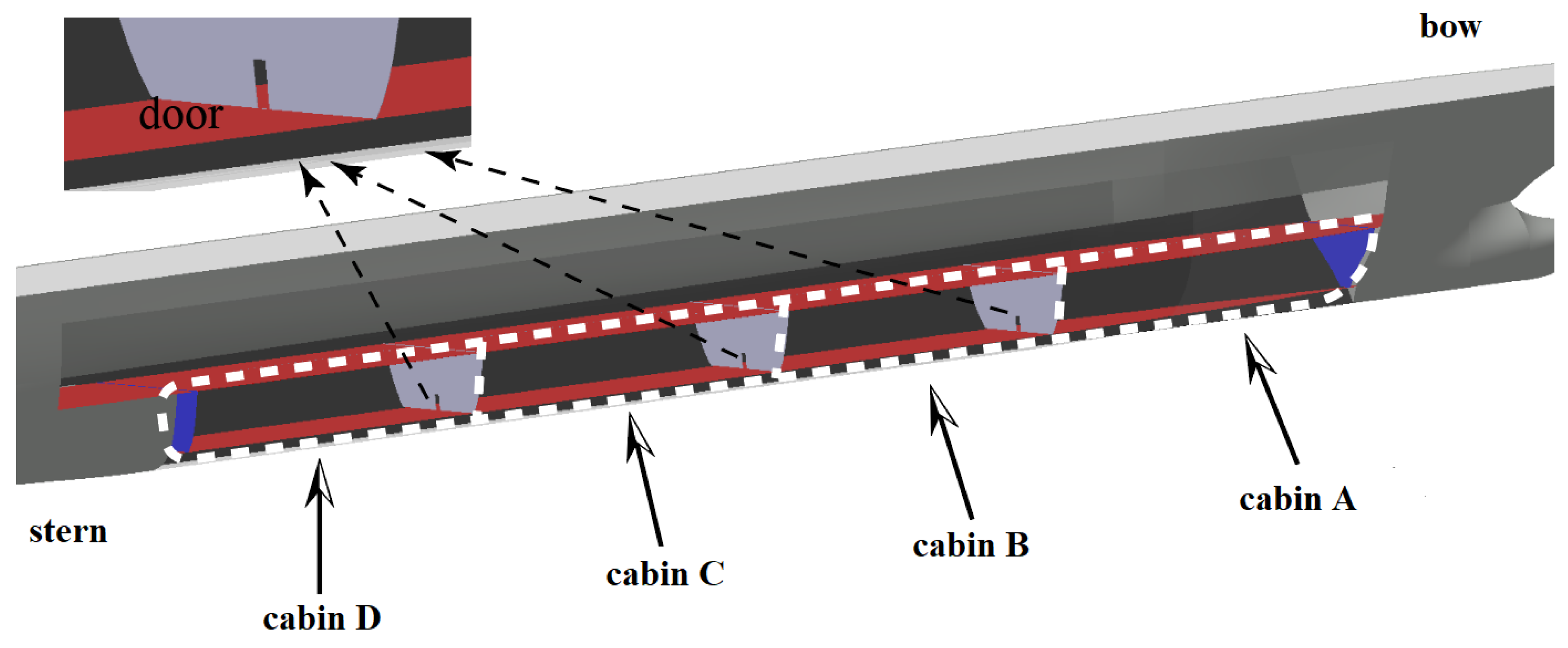
The following scenario was set up in the flooding experiment. Water enters from the damaged compartment and spreads to the four target compartments. These compartments consist of two engine rooms and two ballast tanks. Along the bow-to-stern direction, the two engine rooms are named Compartment A and Compartment B. The two ballast tanks are named compartment C and compartment D (shown in
Figure 5). A total of 272 round holes are made evenly in the bulkheads of the four compartments as the hull damage opening. Only one opening is opened per experiment. Flooding water enters the model ship through the round holes, and then spreads to other compartments through the doors between the compartments. The flooding water eventually covers the four compartments on this deck. For each experiment, the final state of model was not recorded, because whether the ship capsized is not the focus of this paper. In fact, in experiments, the model often does not guarantee complete stability in the end. The model was then elastically fixed using elastic ropes, but this did not cause any restriction on the model’s movement.
The model ship’s damaged opening corresponds to a circular opening with an actual radius of 1.2 m. According to the process in
Section 2.1, a video camera is set up on top of the damaged compartment, which obtains the flooding video when flooding water flows. The remaining compartments do not have any recording equipment. Each compartment is equipped with a flooding alarm at the same height as the door. When the door is flooded, the difficulty of escaping will greatly increase. This is the reason for the selection of the height of the flooding alarm, and it is also the “specified height” in
Section 2.1. Note that a flood alarm and a flood sensor are not the same. The price of the former is much lower than that of the latter.
The opening is blocked before the experiment. When the opening of the model ship is opened, the experiment starts. If the compartment is flooded to the height of the compartment door, the flood alarm will be triggered. The computer will automatically record the time at this time. When the alarms in all four compartments are triggered, the experiment ends. Four compartments’ flooding times are collected. The opening is blocked and the next opening is opened for the next experiment.
In fact, the goal of evacuation decision-making should point to a larger area. Individual compartments that are very close to the opening will be flooded soon after the ship is damaged. There is insufficient meaning for individual compartment’s decisions. Therefore, the flooding area selected in this paper occupies more than 80% of the entire deck space. The four compartments are separated by watertight arrangements. There is only one open watertight door between them. The engine room was chosen because there are usually many crews. These crews all need decision-making information to determine whether to continue anti-sinking operations and when to evacuate.
3.3. Dataset Production
Based on the size of the model ship, 272 holes (of the same size) were opened in the area that may be flooded (the range is indicated by the white dotted line in
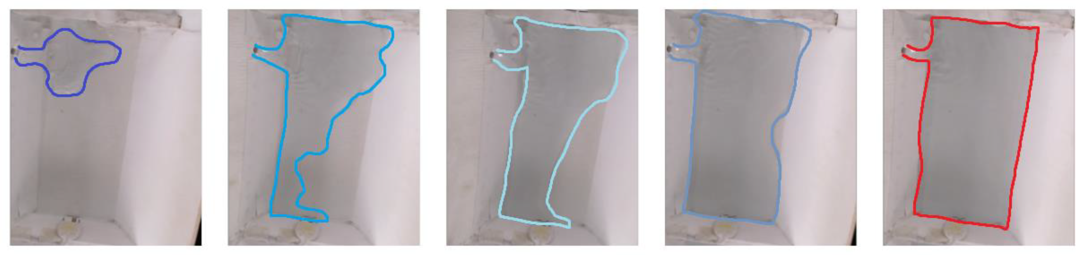
Figure 5 and its symmetrical range, based on the midship longitudinal section). The flooding experiment lasted for one month. The experiment was carried out from ten days in the morning to four in the afternoon every day. Three experiments were carried out for each opening. Each experiment lasted five minutes. The flooding video recording time was two minutes, and the first thirty seconds of the video were used to make the dataset. The video recorded the flooding water of the compartment where the opening is located (
Figure 6). The video was processed into an image at five frames per second using Adobe Premiere Pro. A total of 150 images in PNG format can be obtained from a 30-s video. The size of each image was 1920 × 1440. The whole experiment obtained 816 sets of videos, a total of 122,240 different images. These images were divided into 816 groups according to the ordinal of the opening. Among them, 656 groups were the training dataset. A total of 160 groups was the validation dataset. Its ratio was about 1:4.1. One group corresponded to a flooding scenario, and each flooding scenario needed to predict the flooding time of four compartments. Before entering the neural network, the flooding images do not require any processing. The flooding time needs to be processed as the target manually. For one flooding scenario, there were four compartments’ flooding times as the target. In order to ensure the reliability of the dataset, the proportion of the number of openings in each compartment in the training set was approximately equal to the validation set.
An important aspect of this paper is the production of labels. Note that the problem studied in this paper is distinct from stock forecasting. The neural network does not use the previous value to predict the value in the future. Rather, it is similar to predicting positive or negative comments from viewers based on film reviews. Thus, essentially, the problem studied in this paper is a classification problem, not a regression problem, even if the flooding time is a specific number.
In response to this situation, the researchers found through statistics that all flooding times in the experiment are between 10 s and 130 s. Therefore, the flooding time is discretized and divided into 12 groups with an interval of 10 s: [10,20), [20,30), [30,40), [40,50), [50,60), [60,70), [70,80), [80,90), [90,100), [100,110), [110,120), [120,130). Among them, the flooding time of the three compartments of ABC is no longer than 110 s. The flooding time of compartment D is not less than 30 s, even if the opening is in compartment D. Therefore, the flooding time of the four compartments of ABCD is divided into ten labels. For the flooding time of the ABC compartment, the intervals [10,20), [20,30), [30,40), [40,50), [50,60), [60,70), [70,80), [80,90), [90,100), [100,110) correspond to labels 0–9. For example, the flooding time of 65.30 s is label 5. Similarly, for compartment D, intervals, [30,40), [40,50), [50,60), [60,70), [70,80), [80,90), [90,100), [100,110), [110,120), [120,130), the flooding time is defined as the labels 0–9 in turn.
4. Experience and Discussion
4.1. The Input of Neural Network
The network’s input consists of flooding images. From the decision-making perspective, longer time series flooding images may provide more flooding information, but this will also prolong the time required for decision-making. Too short a flooding image time series can lead to insufficient flood data collection. This can cause the neural network to misjudge flooding development. In the end, an erroneous prediction is given out or even result in a failed prediction.
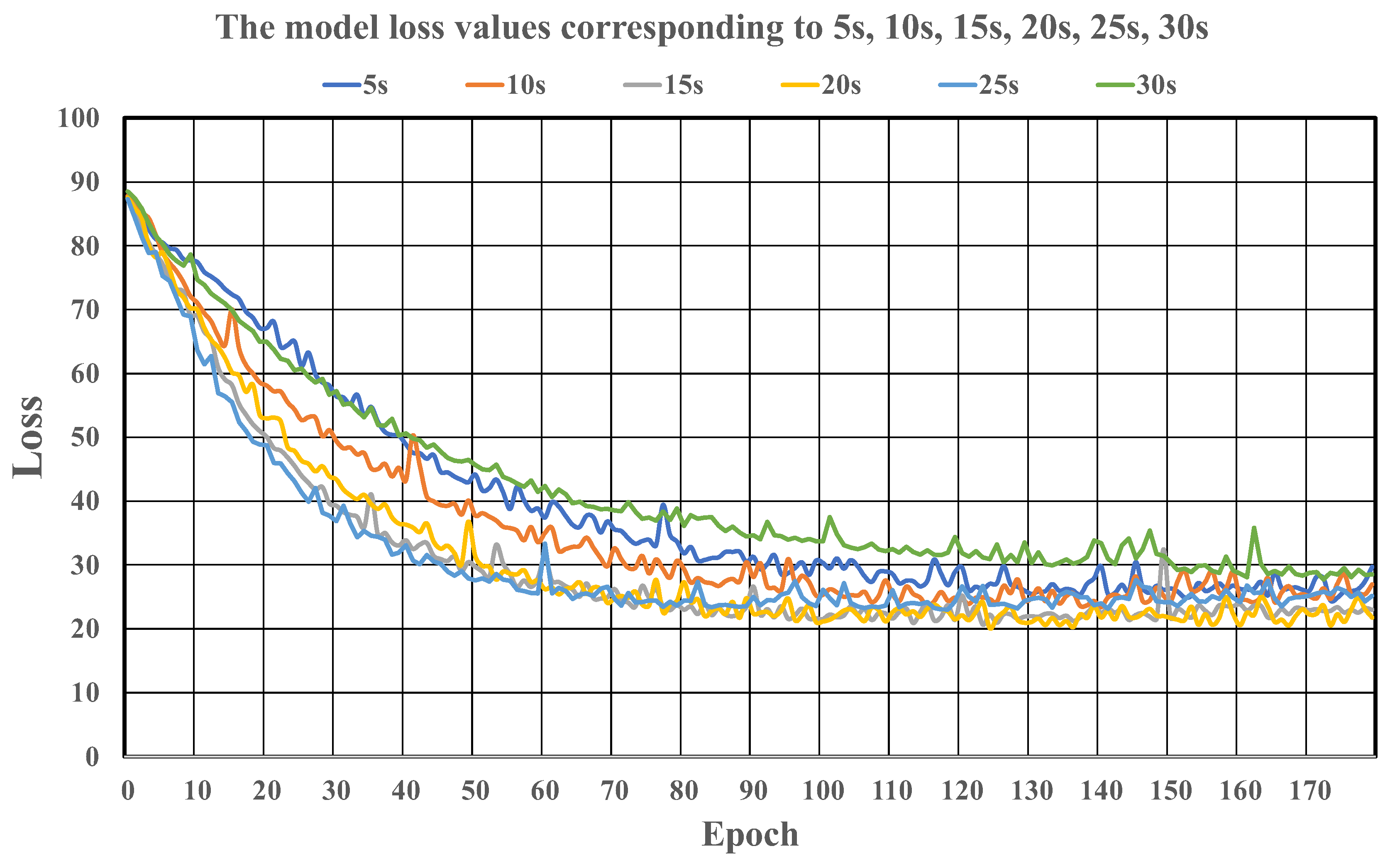
In this paper, six kinds of flooding images with different durations were chosen to determine the appropriate input data. These lengths of time were 5 s, 10 s, 15 s, 20 s, 25 s, 30 s, after the inundation of the model ship. According to the calculation in 2.2, six kinds of times correspond to 70.7 s, 141.4 s, 212.1 s, 282.8 s, 353.5 s, and 424.2 s, respectively, after the flooding of the cruise ship.
The neural network has 180 epochs for each input, the batch size is 16, and one epoch verities 160 datasets.
The total loss value corresponding to the six input durations is shown in
Figure 7. To obtain the total loss value, we sum the individual predicted loss values of the four compartments. The cross-entropy loss function gives single compartment loss.
Figure 7 shows that when the input flood image duration is 30 s, after 80 epochs, the neural network’s loss value is consistently higher than other inputs. Although the thirty second input provided the most flooding information, it was not optimal for the neural network’s rate of convergence and loss value.
Six different inputs, the minimum loss value, and the corresponding iteration steps are shown in
Table 3.
Given the information from
Figure 7 and
Table 2, considering the speed of convergence and the minimum loss value of the neural network, two input durations of fifteen and twenty seconds are better than other inputs. If adding the flooding time, 15 s is ultimately determined to be the most appropriate flooding input duration. The number of epochs is 140.
4.2. Time Accuracy
After the input time is determined, based on this, the prediction accuracy rate of the flooding time under 160 flooding scenarios in the validation dataset can be computed. It is necessary to predict the flooding times
Tpred of the four compartments in each flooding scenario. The target times
Ttarget are given by the flooding experiments. The timing is accurate to two decimal digits. Equation (11) is the accuracy rate
TACC calculation method:
According to the position of the damaged opening, 160 flooding scenarios in the validation dataset were divided into four categories. There are 41 groups, 37 groups, 41 groups, and 41 groups for opening in compartments A, B, C, and D, respectively. For every compartment of the flooding scenario, bring
Tpred,
Ttarget into Equation (11). The summarized results can be divided by the number corresponding to the categories. The average time accuracy of each compartment under different scenarios,
TAcc-A,
TAcc-B,
TAcc-C,
TAcc-D, is obtained, and the results are shown in
Table 4. For example, for the opening in compartment A, by bringing 41 prediction time and 41 target time into Equation (11), we obtain 41 numbers. Then, we calculate the average of 41 numbers, which is the
TAcc-A.
Table 3 shows that regardless of the location of the opening, for the prediction of compartment flooding time, the accuracy exceeds 85%. In most cases, the flooding time prediction rate is more than 91%. This result can better support anti-sedimentation decision-making and help decision-makers have an intuitive understanding of the flooding process. Because the flooding time for each compartment is determined, the escape time of the trapped crew is also determined. Escape time is also useful for decision-makers for planning evacuation routes based on the degree of urgency and cooperating with various on-board rescue equipment to increase the likelihood of the escape of the trapped crew. If a rescue force is added, the escape time will only be prolonged.
However, the accuracy of predicting the flooding time of the compartment where the opening is located is lower than other compartments. This is due to the fact that the compartment where the opening is located is almost always the first to reach the warning water level. The amount of time used for flooding will be less than other compartments. As per Equation (11), when the whole flooding process is not long, the shorter the flooding time, the greater the error.
When the opening is located at compartment D, the prediction time accuracy of compartment D approaches that of the other compartments. This prediction accuracy is different from other situations where the opening is in intact compartments. Due to the larger volume of compartment D, it takes a longer time to reach the warning height. In fact, when the opening is in compartment A, the time for compartment A to reach the warning water level will be no more than 20 s, and when the opening is in compartment D, the flooding time of compartment D to reach the warning line is at least 35 s.
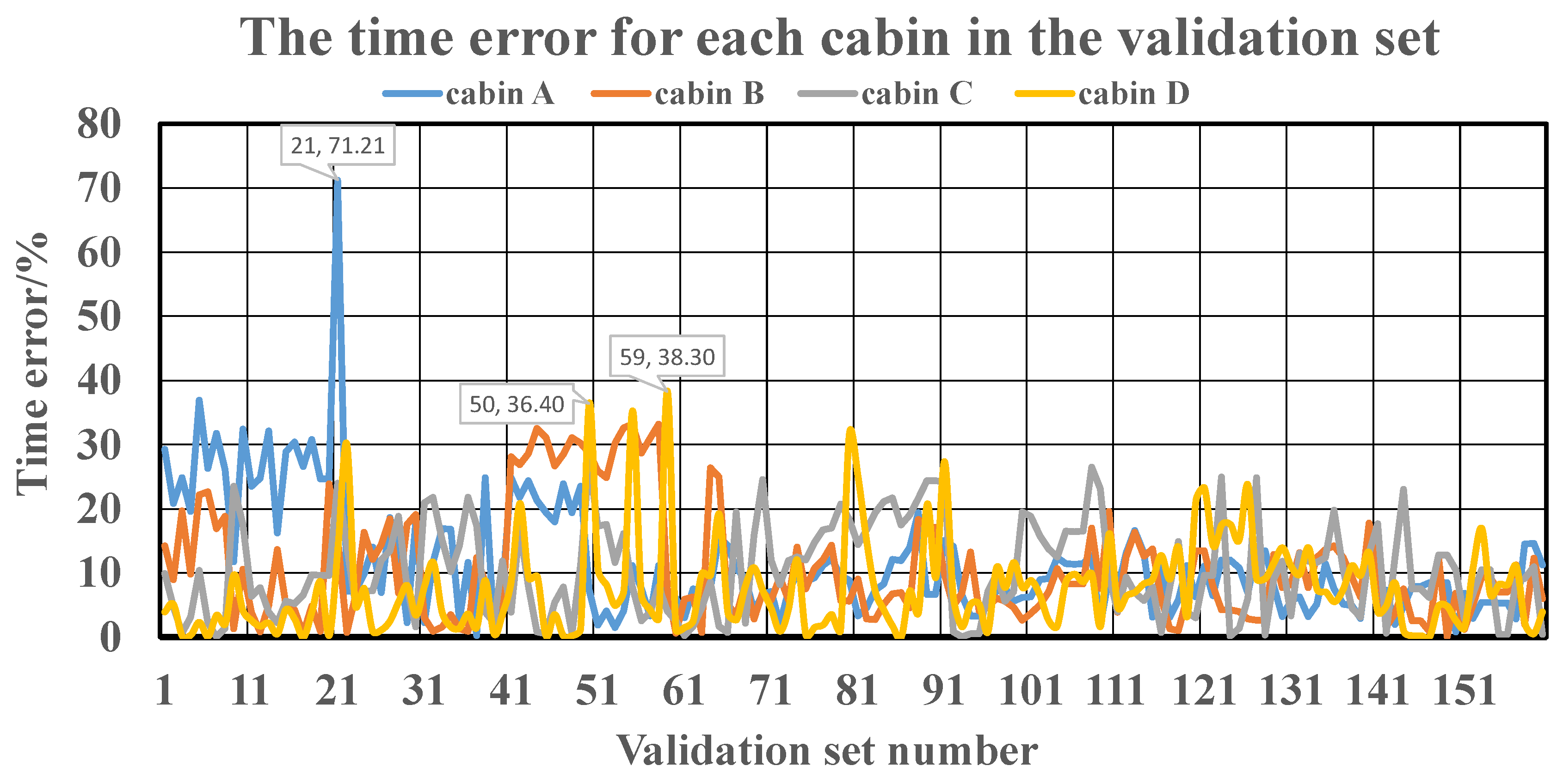
For all the flooding scenarios in this paper, the time error percentages for each compartment were calculated. They are presented in
Figure 8.
The cases where the neural network prediction error exceeds 35% were sorted out, and they appear in compartment A of the 21st flooding scenario, and compartment D of the 50th and 59th flooding scenarios. For these flooding scenarios, the target flooding time and predicted time of the cruise ship were calculated using the conversion coefficient C, shown in
Table 5.
From the view of a cruise ship, even if the neural network prediction has an error of more than 35% in individual cases, the difference between the prediction result and the real time does not exceed 9 min. Especially in flooding scenarios of 50 and 59, the flooding water is poured in from the B compartment, which gives more time for the trapped crewmembers in the D compartment.
4.3. Decision Making
After a ship is damaged, flooding information can be obtained effectively according to the prediction results given by the composite neural network. The flooding scenario with the largest error in
Table 4 was selected to illustrate the extreme effect of the composite neural network, namely, scenario 21 of flooding. In addition, according to the accuracy rate in
Table 3, the situation where the opening is in compartment D was also selected, to show the overall effect of the composite neural network’s prediction.
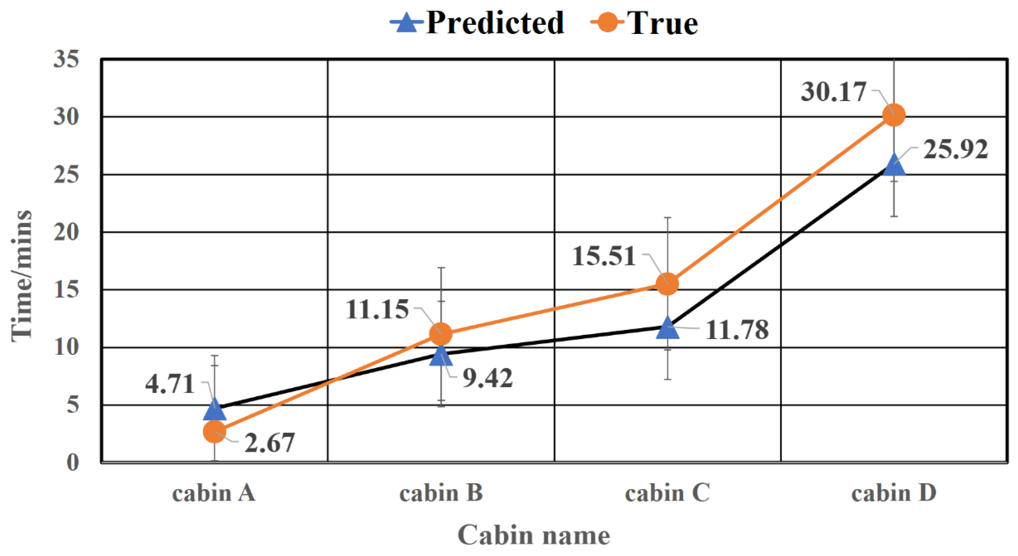
For flooding scenario 21, the following are the results of this flooding experiment: the times for the four compartments of the model ship to reach the warning water level are 11.35 s, 47.33 s, 65.83 s, and 128.04 s. The neural network predicts 20 s, 40 s, 50 s, 110 s, respectively. Since the flooding time of the model ship is too short, for the sake of intuition, we observe from the perspective of a cruise ship. The flooding experiment results that correspond to the cruise ship times are 2.67 min, 11.15 min, 15.51 min, and 30.17 min. The neural network prediction results correspond to the cruise ship times of 4.71 min, 9.42 min, 11.78 min and 25.92 min.
Figure 9 can be produced from this. The red curve is the time predicted by the composite neural network. The black curve is the real time obtained from the flooding experiment. Time data was combined with the time conversion coefficient C. Note that the prediction effect of the neural network is observed from the cruise ship’s perspective, which does not mean that the composite neural network trained with the dataset in this paper can be directly applied to the real ship.
From
Figure 9, it can be found that the error between the predicted and target time of compartment A is 2.04 min, and the errors of compartment B, compartment C, and compartment D are 1.73 min, 3.73 min and 4.15 min, respectively. The time accuracy rates are 28.79%, 85.49%, 76.96%, and 86.25%. Compared with the evacuation time of more than ten minutes, the error of the compartments of BCD is acceptable. Poor time prediction results for compartment A. However, the prediction error of compartment A belongs to the only example in the 160 sets of data. Moreover, this is the flooding scenario with the largest error in the entire validation dataset. The errors of other flooding scenarios are much smaller than this data, as shown in
Figure 8.
In addition, as the development of flooding event, the flooding time predicted error is bigger and bigger. This means that the mastery of flooding by neural networks decreases as the flooding spreads. Intuitively, the error bars in
Figure 9 gradually increase.
After flooding occurs, the order of the four compartments arriving at the warning line is A, B, C, D. That is, after flooding, the evacuation time for the crew in compartment A is the shortest, and the decision-maker must give the escape route as soon as possible according to the structural diagram of the ship. That is, they must transfer to the adjacent compartment B or to a higher deck within 4.71 min. The crew of compartments B and C need to leave compartment B and compartment C within 9.42 min and 11.78 min, respectively. The trapped crew members in compartment D need to be rescued or evacuated to a higher deck within 25.92 min. The trapped crew members need to decide the next behavior based on the evacuation information given by the neural network, and the rescuers need to save the most trapped crew within this time or extend the maximum rescue time through the drainage equipment on the ship.
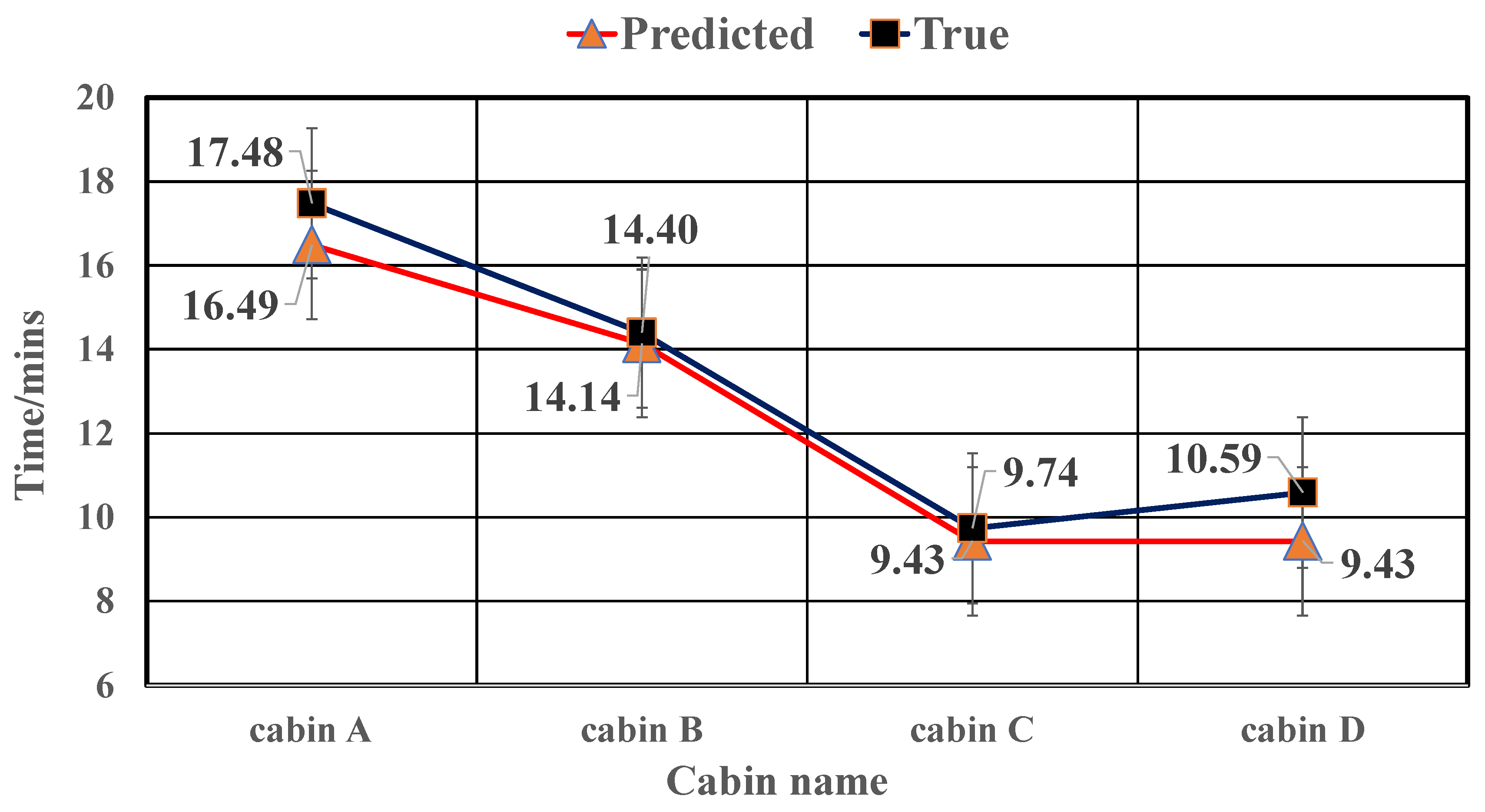
Similarly, flooding scenario 131 (opening in compartment D) is chosen to illustrate the overall level of neural network prediction performance.
Figure 10 was also made according to the predicted time and the real flooding time. The black curve represents the physical experiment results, and the red curve represents the neural network prediction results. When both of them undergo the conversion coefficient C, the observation angle is changed from the model ship to the cruise ship. It is calculated that the time accuracy rates of the A, B, C, D four compartment predictions are 94.34%, 91.82%, 96.74%, and 89.91%, respectively. This example shows the overall prediction effect of the neural network. From the black curve in
Figure 10, the sequence of flooding water reaching the warning line is compartment C, compartment D, compartment B, and compartment A. The time in compartment C and compartment D is very close, with a difference of only 0.85 min. This shows that after the water entered from compartment C, it quickly spread to compartment D. This feature is also reflected in the prediction, that is, the neural network gives 9.43 min for the two compartments of C, D to reach the warning line.
From
Figure 10, it can be found that the errors between the forecast and actual results of the four compartments are 0.99 min, 0.26 min, 0.29 min and 1.16 min, respectively. This result is very satisfactory. This means that the decision-maker can obtain more accurate flooding information of the target compartment shortly after the flooding occurs. The flooding development trends of these compartments can be well-predicted and grasped, which is undoubtedly conducive to reasonable decision-making. In fact, the prediction level of the neural network similar to flooding scenario 131 is the average level.
4.4. The Accuracy between the Model and the Real Ship
Theoretically, the training of neural networks for real ships is consistent with the model mentioned in the paper. Considering the following method: for different scale models (1:200, 1:100, 1:150, etc.), the same method is used to train neural network, each model-trained neural network will give a time prediction for the same flooding scene (only the cabin size is different). Comparing the relationship between prediction times for different scenarios, further exploration is made for the influence of scale-in ratios on prediction results. Finally, a reliable training strategy can be used in real ships.


