Abstract
Marine heatwaves (MHWs) are becoming increasingly frequent and intense around China, impacting marine ecosystems and coastal communities. Accurate forecasting of MHWs is crucial for their management and mitigation. In this study, we assess the forecasting ability of the global eddy-resolving ocean forecast system LICOM Forecast System (LFS) for the MHW events in October 2021 around China. Our results show that the 1-day lead forecast by the LFS accounts for up to 79% of the observed MHWs, with the highest skill during the initial and decay periods. The forecasted duration and intensity of the MHW event are consistent with observations but with some deviations in specific regions of the Yellow and South China seas. A detailed analysis of the heat budget reveals that the forecasted shortwave radiation flux is a key factor in the accuracy of the forecasted MHW duration and intensity. The oceanic dynamic term also greatly contributes to the accuracy in the southern Yellow Sea. In addition, the increasing bias of the forecasted duration and intensity with lead time are mainly caused by the underestimated shortwave radiation. Our findings suggest that improving the accuracy of oceanic dynamic processes and surface radiation fluxes in the LFS could be a promising direction to enhance the forecasting ability of marine extreme events such as MHWs.
1. Introduction
Marine heatwaves (MHWs) are prolonged high-temperature events characterized by a sea surface temperature (SST) exceeding a certain threshold for several days to months and covering thousands of square kilometers in spatial extent [1,2,3]. In recent years, MHWs have become increasingly frequent and intense, particularly in the context of global warming, resulting in severe impacts on ecology and human society. These sustained high temperatures have dire consequences on marine organisms and ecosystems, as well as leading to significant economic losses in industries, such as seafood and aquaculture [4,5,6,7]. Specifically, in marginal seas, such as the China Sea, the sustained high temperatures have dire consequences on marine organisms and ecosystems, leading to mass die-offs of species, changes in biodiversity, and the emergence of harmful algal blooms. Furthermore, MHWs can cause significant economic losses in industries, such as seafood and aquaculture, as well as affecting human health through the spread of diseases and toxins locally.
MHW research has gained substantial attention in recent years, focusing on three key areas: detecting MHWs, understanding the physical mechanisms driving MHWs, and predicting MHWs [8]. There are various definitions for determining MHWs, including using a temperature threshold of 2 °C to 5 °C above the climatic mean or maximum temperature lasting at least three to five days [9,10,11], as well as using a percentile threshold and requiring more than five days above the threshold [12,13].
MHWs are directly caused by net surface heat flux anomalies, which occur when the mixed-layer depth becomes shallow and allows the warm anomaly signal to penetrate the deep layer due to mixing, rapidly developing the event [14]. Several factors contribute to these heat flux anomalies, including non-local sea surface temperature anomalies (SSTAs) that impact local atmospheric circulation fields [15], sea-ice melting [16], cloud–radiation feedback [17], and El Niño [18]. Research has also considered the impact of non-local salinity anomaly transport on the generation of MHWs, which alters the density and changes the mixed layer in the northeast Pacific [19]. Yan et al. [20] pointed to increased solar radiation and weaker winds in the Yellow and East China seas, separated from the western Pacific subtropical high, as the primary causes of MHWs in 2004, 2006, and 2016. These findings suggest that different processes dominate the generation and sustaining of MHWs in various regions and periods.
The potential predictability of MHWs is still a challenge. Behrens et al. [21] identified ocean heat content as a prerequisite for MHWs and found that the predictability is on the timescale of weeks. Jacox et al. [22] showed that climate models can provide accurate seasonal forecasts of MHWs that are long-lived events (>1 month). However, the current forecasting systems for short-lived MHW events still need more research, especially on the weather scale. It is worth investigating the capacity of real-time operational forecast systems to predict MHWs on the regional scale and the weather scale.
This study aims to assess the performance of a global eddy-resolving marine environmental forecasting system in predicting MHW events on the weather scale, and to identify possible causes of forecast biases. Our analysis focuses on the MHW event that occurred in marginal seas around China from September to October 2021, which coincided with the beginning of a strong La Niña event that lasted until the end of 2022. The combination of these factors makes this particular MHW event an excellent case study for evaluating the forecast system’s performance under the influence of large-scale climate variability. The insights gained from this research will provide valuable guidance for improving the forecasting accuracy of such events in future work. The second part of this paper describes the methodology, observational data, and the global marine environmental forecasting system used in this study. The third part presents an analysis of the characteristics of an MHW event, the performance and bias of the forecasting system, and the causes of the forecast bias. Finally, the paper concludes with a summary and discussion of the results.
2. Data and Methods
2.1. LICOM Forecast System Data
The forecast data used in this paper are sourced from the LICOM Forecast System (LFS), a global high-resolution marine environment forecasting system in China [23]. The LFS utilizes the LICOM model, a global ocean circulation model developed by the Ocean Model Team of the State Key Laboratory of Numerical Modeling for Atmospheric Sciences and Geophysical Fluid Dynamics (LASG), the Institute of Atmospheric Physics (IAP), Chinese Academy of Sciences (CAS). The finite difference method is employed to numerically solve the primitive equation, continuity equation, seawater state equation, and temperature–salt conservation equation, subject to given initial and boundary value conditions.
The latest version of LICOM (LICOM 3.0) was developed into a global eddy-resolving ocean circulation model with a horizontal resolution of 1/10°. It participates in the International Ocean Model Intercomparison Program (OMIP) and achieves good results [24,25,26,27], including the western boundary regions [25]. Furthermore, LICOM 3.0 has a set of sub-versions, with different resolutions and parameterization schemes, in which the highest resolution reaches 3–5 km [28]. LFS was developed based on LICOM 3.0 for short-term (1–7 days) and medium-term (7–30 days) marine environment forecasting.
LFS consists of two main modules: a data assimilation analysis module and a forecast module using the LICOM 3.0 model with a horizontal resolution of 10 km and a vertical layer of 55 layers. The data assimilation analysis module obtains the initial forecast value using the observation data nudging method. The forecast model is driven by the Global Forecast System (GFS) atmospheric forcing field from the National Centers for Environmental Prediction (NCEP). LFS can predict the marine environment for 1–15 days. The forecast variables include sea surface height, three-dimensional temperature, salinity, and ocean currents.
LFS underwent an operational trial operation at China’s National Marine Environment Forecast Center from August to December 2020. During this period, the 1-day lead SST forecast had a root mean square error (RMSE) of 0.604 °C, and the RMSE of the temperature and salinity profiles was 0.563 °C and 0.098 PSU, respectively. More information about LFS can be found in Liu et al. [23] and Zheng et al. [29].
2.2. Observational Data
The daily SST data used in this study are from the daily Optimum Interpolation Sea Surface Temperature (OISST) dataset provided by the National Oceanic and Atmospheric Administration (NOAA) [30,31,32]. This dataset has a spatial resolution of 0.25° × 0.25° and covers the period from 1 September 1981 to present. To evaluate the ability of the LFS system to forecast MHWs, we use the daily SST data from 1 January 1982 to 31 December 2021. This dataset is used as the reference of SST, which provides the reference of MHWs.
In this study, the European Centre for Medium-Range Weather Forecasts (ECMWF) Reanalysis v5 (ERA5) data [33] are used to investigate the forecast of heat flux. The dataset has a spatial resolution of 0.25° and a daily temporal resolution, which enables a comprehensive understanding of heat flux in the study region. The daily ERA5 data from 1 September to 31 October 2021 are used to evaluate the predicted latent heat and shortwave radiation.
2.3. Definition of MHW Events
The threshold used to define MHW events is a critical criterion. In earlier studies, a fixed threshold was commonly used [34], but this is suitable only for areas with relatively small-latitude spans. The percentile threshold method was recently adopted [12]. This method calculates the 90th percentile of the daily temperature based on all years and smooths it over 31 days. The new definition of an MHW event includes anomalous warming events that last five days or longer, with daily mean SSTs above the 90th percentile over a 30-year historical baseline. The threshold method can simultaneously consider temporal and spatial variation. The Hobday et al. [12] method has been widely used in recent studies.
In our study, we slightly modified the definition of an MHW event used by Hobday et al. [12] in two ways. First, we used the 95th percentile (Equation (1)) as the threshold for the China Sea, which is more stringent than the 90th percentile used by Hobday et al. [12]. Second, we did not perform any temporal smoothing before obtaining the threshold. This approach produces a more realistic threshold, as smoothing can artificially affect the intensity and duration of MHW events.
The threshold for MHW events is calculated based on the SST from the OISST dataset between 1982 and 2021. For each grid point, the SST on a given date (t) for all 39 years is sorted from low to high. The threshold value is then determined as the 95th percentile of the sorted SST values for the corresponding date and grid point. For example, the threshold value for the grid point (x, y) on a date (t) is calculated as follows:
In the formula, is the 95th percentile of SST for the date t and is SST value in the kth year. The threshold value varies in both space and time, as it changes with the grid point and date. Moreover, the duration of extremely high SST is also an essential indicator for MHW events. Therefore, in this study, an MHW event is defined as a consecutive period of at least five days with SST greater than the threshold value for each grid point.
MHW events are characterized as extreme events by their occurrence position and date, duration time, and intensity. The occurrence position and date can be evaluated by comparing the percentage of the MHW occurrence area to that of the observations. Duration time is the total time covering the start and end dates of an MHW event and is longer than or equal to five days according to the definition in our study. The definition of intensity refers to the maximum SST exceeding the threshold for an MHW event. Our analysis focuses on the MHW event that occurred from September to October 2021, which coincided with the beginning of a strong La Niña event. The combination of these backgrounds makes this particular MHW event an excellent case study for evaluating the forecast system’s performance under the influence of large-scale climate variability.
2.4. Statistical Metrics
Three metrics based on SSTA are used to examine the bias between the observed and forecasted results. The first metric, the mean absolute error (MAE), assesses the deviation between the observed and forecasted results and is defined by computing the difference between the forecasted SST on a particular date and the corresponding climatological daily OISST SST for that date. The formula is as follows:
where represents the forecasted SSTA at the grid , represents the observed SSTA from the OISST, is the area weight at the grid , and and are the total number in the longitude and latitude directions in the whole region, respectively.
The second metric, RMSE, evaluates the bias between the observed and forecasted results by taking the square root of the sum of the squared differences between forecasted and observed SSTA. The formula is as follows:
where , , and are the same as those in the MAE equation.
The third metric, PCC, evaluates the spatial correlation between the observed and forecasted results by computing the correlation coefficient between the two. For example, the PCC between the OISST and the 1-day lead forecast is defined as follows:
where and are the same as those in the MAE equation. represents the mean 1-day lead forecasted SSTA in the whole region and represents the mean SSTA from the OISST.
Two metrics based on MHW events are also used to assess the skill of the LFS predictions. The first metric is the area ratio, which measures the proportion of the region where LFS predicts an MHW event relative to the observed MHW event area. Specifically, the area ratio for the 1-day lead forecast is defined as follows:
where represents the area where an MHW event occurs in the 1-day lead forecast and represents the area of an MHW event in the OISST.
The second metric is the Symmetric Extremal Dependence Index (SEDI), which is used to evaluate the forecasting ability of LFS. SEDI is defined based on a 2° × 2° contingency table [35].
where H = a/(a + c) is the hit rate and F = b/(b + d) is the false-alarm rate. a, b, c, and d are the total hits, false alarms, misses, and correct rejections in a 2° × 2° contingency table. The values for a, b, c, and d here are calculated as to whether the proposed criterion satisfies the grid of LFS. Hits (a) represent that the MHW occurs in the same grid in both the OISST and LFS. False alarm (b) represents that the MHW occurs in the LFS grid but not in the OISST. Misses (c) represent that the MHW occurs in the OISST grid but not in LFS. Correct rejections (d) represent that the MHW does not occur in the grid in both the OISST and LFS. The value of SEDI ranges from −1 to +1, and positive, larger values indicate better skill of the forecast system [35,36].
2.5. Heat Budget of SST
SST is the determining variable for the definition of MHWs. The local variation in SST in the ocean is mainly influenced by the ocean dynamics term and the net surface heat flux. The ocean dynamics term includes temperature advection, horizontal and vertical temperature diffusions. The net surface heat flux includes net shortwave radiation, net longwave radiation, latent heat, and sensible heat. Those enter the forecast system through the forcing field. Therefore, the SST governing equation [37] can be formulated as a balance of the above terms, which is as follows:
where T is the averaged ocean temperature in the first layer depth of the ocean model, and are the horizontal and vertical temperature advection, respectively, and is the sum of the above two terms, referred to as the ocean dynamics term. here is vertical velocity at the base of first depth of ocean model. , , , and represent the shortwave radiation flux, longwave radiation flux, latent heat flux, and sensible heat flux, respectively. is the density () and is constant-pressure specific heat capacity for seawater (). here uses the thickness of the first layer in the ocean model, so the influencing factors of shortwave radiation, longwave radiation, latent heat, and sensible heat can be expressed in simplified forms , , , and . The diffusion of heat has been neglected [36]. To sum up, the SST budget is mainly composed of two parts: the ocean dynamics term and the net heat flux term, which includes shortwave radiation, longwave radiation, latent heat, and sensible heat. Based on Equation (7), is chosen as one day here, and is multiplied on both sides of Equation (7) to display the SST budget with the unit of temperature. The equation is transformed as follows:
In this study, we utilize the following variables: SST, SW, LW, LH, and SH. Additionally, the is calculated as the residual between ∂T and the surface heat flux. All of the variables employed in this research are obtained from the LFS output, which has a daily temporal resolution and a spatial resolution of approximately 10 km.
3. Results
3.1. Evolution of the MHW Event
This study uses the 95th percentile of SST as the threshold for defining the MHW event around China. To validate the effectiveness of this threshold, we selected four sites (120° E, 38° N), (122° E, 35° N), (123° E, 28° N), and (115° E, 20° N) in the Bohai Sea, Yellow Sea, East China Sea, and South China Sea, respectively (Figure 1a). Figure 1b–e show the probability density functions (PDFs) of the observed SST at four points using the daily mean SST during 1982–2021 from the OISST dataset. We find that they all generally exhibit a normal distribution. The values of the 95th percentile of SST at the four points are 22.0 °C, 22.4 °C, 26.4 °C, and 28.8 °C, respectively. Thus, the 95th percentile of SST is a valid threshold for defining the MHW, as extremely high values are detected in different regions.
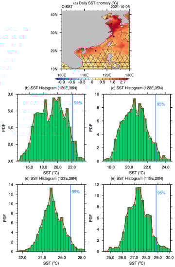
Figure 1.
SSTA on 6 October 2021 and PDFs of the SST for four representative sites in the China Sea. (a) The shaded areas show the SSTA based on daily OISST data from 1982 to 2021, with unmasked areas indicating the regions where SST reaches the definition of an MHW. The four selected sites in the Bohai Sea, Yellow Sea, East China Sea, and South China Sea are marked as black dots. (b–e) The PDFs of the SST in October at these sites, with the red dashed lines representing the PDFs and the blue vertical lines marking the threshold value defined by the 95th percentile value.
Figure 2 shows the time series of observed daily SST, the MHW threshold, and the climatological daily SST at the four sites from 1 September to 31 October 2021. At these sites, the threshold for the MHW is 1.5–2 °C higher than the climatological daily mean value. The SSTs at these sites exceeding the threshold are indicated by pink shading. We find that SSTs higher than the threshold mainly occur in the Yellow Sea (Figure 2b) and the East China Sea (Figure 2c). According to the criterion of the lasting time, the period of high SST must last at least five days; thus, the MHW event is further confirmed. There are two MHW events for the point in the East China Sea (Figure 2c) at the beginning of September and the beginning of October. For the points in the Yellow Sea (Figure 2b) and the South China Sea (Figure 2d), only one MHW event occurred around 1 October. Here, we only focus on the MHW event that occurred from late September to mid-October.
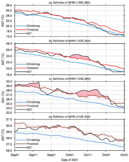
Figure 2.
(a–d) The temporal evolution of the daily SST, the climatological SST, and the MHW threshold at the four representative sites (marked as black dots in Figure 1a) in the China Sea from 1 September to 31 October 2021. The blue lines represent the climatological SST from 1982 to 2021, based on the OISST dataset. The red lines represent the threshold value of an MHW, defined based on the 95th percentile value of the SST. The black lines show the daily SST at the four sites, also obtained from the OISST dataset. The pink areas indicate when the SSTs reached or exceeded the MHW threshold.
Figure 3a–e show the evolution of this MHW event around China based on the SSTA distribution and the occurrence of the MHW on 20 September, 30 September, 6 October, 12 October, and 22 October 2021. The SSTA is used to depict the development of the MHW event, with the unmasked area indicating values higher than the MHW criterion. It provides a depiction of the different stages of the MHW event around China (based on the ratio of the occurred area to the whole area), including the initial state (below 10%), development state (10–40%), mature state (40–100%), decay state (10–40%), and extinction state (below 10%). In the initial phase, the MHW event appears first in the Taiwan Strait and its western side on 20 September. The event then expanded northward, dominating the northern South China Sea and the Yellow Sea on 30 September. The peak of the MHW event occurred on 6 October, covering almost the entire China Sea, with a total area of 2.08 × 10⁶ km2. However, the area of the MHW event began to shrink after 6 October, and by 12 October, it occurred only in the northern South China Sea, the Yellow Sea, and the East China Sea. Finally, on 22 October, the MHW event appeared only in a small region of the East China Sea, which lasted for about a month. This case in Figure 3a–e provides an observational reference for evaluating the forecasted MHW event around China.
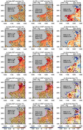
Figure 3.
Spatiotemporal evolution of SSTA and occurrence of the MHW in the observations (OISST) and the 1-day lead forecast (LFS). The left column (a–e) depicts the SSTA observed by OISST and the middle column (f–j) depicts the 1-day lead forecast of SSTA from LFS. The unmasked areas in (a–e) and (f–j) indicate where the SST reaches the definition of an MHW in OISST and LFS, respectively. The right column (k–o) shows the difference in SSTA between the OISST and LFS. The (a,f,k), (b,g,l), (c,h,m), (d,i,n), and (e,j,o) represent 20 September, 30 September, 6 October, 12 October, and 22 October, respectively. The SSTA is calculated by subtracting the climatological daily SST during 1982–2021 from the OISST. The mean, maximum, and minimum SSTA values in the study area are denoted, along with the PCC, SEDI, and ratio. The MAE and RMSE between the OISST and LFS are also shown in the right column.
The 1-day lead forecasted SSTAs from LFS are shown in Figure 3f–j. Three metrics were applied to evaluate the forecast skill of the MHW structure: PCC, area ratio, and SEDI. The definition and equations to calculate these indices can be found in Section 2. The results show that the LFS forecast has varying skill in reproducing the different phases of the MHW event. During the initial phase, the LFS forecast has a PCC of 0.41 for the SSTA and a ratio of 65% for the MHW event on 20 September. SEDI during this phase is 0.59, which is just above the median value. During the development phase, the PCC increases to 0.59, and the area ratio increases to 73% on 30 September. However, SEDI decreases to 0.51, indicating that SEDI is not solely affected by the spatial pattern and the coverage.
During the mature phase, the PCC between the forecasted SSTA and the observation increases to 0.67 on 6 October; the LFS forecast reproduces only 53% of the MHW event. This decrease in performance is due to cold biases in the Bohai Sea and the east of Taiwan Island and false predictions in the South China Sea. SEDI decreases to 0.31 in this phase (Figure 4). Both the area ratio and SEDI indicate a worse forecast skill during the mature phase.
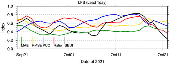
Figure 4.
Temporal evolution of the performance metrics of the 1-day lead forecast by LFS during the duration of the MHW event. The metrics shown are the MAE, RMSE, PCC, area ratio, and SEDI.
During the decay phase, the LFS forecast is closer to the observations, with a PCC of 0.76 and a reproduction of 62% of the MHW event on 12 October. SEDI and the area ratio (0.73 and 79%, respectively) reach their peaks in this phase (Figure 4). However, during the extinction phase, the deviation from the observations increases, with a PCC of 0.53 and a reproduction of only 36% of the MHW event on 22 October. SEDI decreases to its lowest value (0.23) in this phase.
Overall, the results suggest that the 1-day lead LFS forecast can predict the life cycle of the MHW event, with the highest skill for the decay phase compared with the other phases, achieving peak values of 79% and 0.73 for area ratio and SEDI, respectively. The three criteria, PCC, area ratio, and SEDI, are used to evaluate the forecast skill and the time during which these criteria exceeded 0.6 accounts for 67%, 66%, and 42% for the MHW event period, respectively.
The attribution of SEDI is analyzed in Figure 5. SEDI is calculated based on the hits rate (H) and false-alarm rate (F). A comparison between SEDI and its two parts (F and H) shows that the SEDI time series is highly correlated with both the H and F time series (Figure 5a). The correlation coefficients between SEDI and H/F are 0.70/−0.73, both of which are significant at the 95% confidence level. Moreover, H and F are calculated using four parameters: hits, false alarms, misses, and correct rejections, represented by a, b, c, and d, respectively. F is significantly (95%) related to all four parameters, in particular, false alarms (b, 0.89) and correct rejections (d, −0.80). In contrast, the area ratio considers only the situation of the predicted MHW, which is the hits in SDEI. Therefore, SEDI contains all situations (a, b, c, and d), whereas the area ratio represents only the hits rate. This difference may explain why the SEDI time series has different peaks compared with the area ratio.
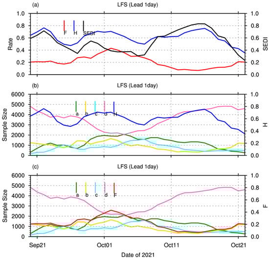
Figure 5.
Evaluation of the 1-day lead forecast of the MHW event by LFS using the SEDI metric. (a) Time series of the SEDI hits rate (H) and false-alarm rate (F) over the MHW event period. (b) Time series of hits, false alarms, misses correct rejections, and hits rate (H). (c) Time series of hits, false alarms, misses correct rejections, and the false-alarm rate (F).
The SST difference analysis (Figure 3k–o) reveals that the SST biases for 1-day lead forecasts by LFS can impact the prediction of the MHW event, since the definition of MHW is based on SST. For instance, the Bohai Sea shows a consistent cold bias throughout the entire period. In contrast, the southern part of the Yellow Sea exhibits a cold bias only during the mature period. The SSTA biases are consistent with the biases in the occurrence of the MHW event, highlighting the need to consider the SST difference when evaluating the forecast skill of LFS. By identifying the biases in LFS, we can further understand the evolution of the MHW event in the system.
In Figure 6, the distribution of the SSTAs and the occurrence of the MHW event during the mature phase (6 October) obtained from the OISST and LFS 1-day, 6-day, and 11-day lead forecasts are presented. The 1-day lead forecast captures 53% of the observed MHW event area (unmasked in Figure 6b), approximately 1.95 × 10⁶ km2. The forecast cold errors are evident in the Bohai Sea, where the observed MHW event is not captured (misses, masked blue). The analysis in the following section (Section 3.2) reveals that the bias may be caused by the weakening shortwave radiation in the area from 4 October. Another error is the false alarms (masked green) in the northern South China Sea.
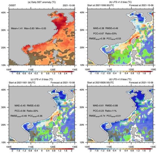
Figure 6.
Comparison of SSTA and occurrence of MHW event between the OISST and LFS forecasts. (a) SSTA (shaded) and occurrence of the MHW (unmasked) from the OISST on 6 October 2021. SSTA is relative to the climatological daily SST during 1982–2021 from the OISST. The mean, maximum, and minimum of the SSTA in the whole area from the OISST are indicated. The occurrence of the MHW indicates that the SST reached the definition of an MHW. (b–d) SSTA biases (shaded) and the hits (unmasked), false alarms (masked green), misses (masked blue), and correct rejections (masked black) for the 1-day lead, 6-day lead, and 11-day lead forecasts on 6 October by LFS, respectively. The area–weight MAE, area–weight mean RMSE, PCC between the OISST and LFS, and the area ratio of the forecasted MHW occurrence to that in OISST are also indicated. and represent the area-weight mean RMSE and PCC in the unmasked area (a). Units: °C.
In general, the 1-day-lead-predicted SSTA (Figure 6b) shows a high spatial correlation with the observed SSTA (Figure 6a), with a correlation coefficient of 0.67. The mean RMSE for the entire region is 0.49 °C, indicating a relatively high forecasting skill for LFS. However, the 1-day-lead-predicted SSTA in the Bohai Sea is relatively cold, leading to a missed prediction of the MHW event in this area. Conversely, the predicted SSTA near Taiwan Island and the northern part of the South China Sea is warmer than OISST SSTA, resulting in stronger predicted intensities of the MHW event, which is displayed in Figure 10.
The forecasted occurrence of the MHW event at 6-day lead and 11-day lead on 6 October (as shown in Figure 6c,d) showed a poorer forecast skill than the 1-day lead forecast, with the ratio decreasing from 53% to 11% with lead time. Other evaluation criteria, including PCC and RMSE, also showed decreased forecast skill with lead time. The reduction in forecast skill is primarily attributed to the missed predictions by LFS, as evidenced by the rapidly growing blue masked area (representing misses) with lead time in Figure 6.
Figure 7 illustrates the changes in MAE (blue curve), RMSE (orange curve), PCC (grey curve), and the area ratio (yellow curve) as the forecast lead time increases from 1 day to 15 days. The results indicate that the forecasting skill tends to deteriorate as the forecast lead time increases, mainly when the lead time is less than ten days. However, that relationship becomes less significant when the lead time exceeds seven days. For example, the value of the area ratio oscillates around 30% when the lead forecast time is longer than seven days. These results suggest that the LFS has a high forecasting skill in MHW events within lead times of less than a week. Moreover, the analysis of different types of predicted error (as shown in Figure 6, masked area) reveals that misses are the main factor contributing to the decreased forecasting skill with increasing lead time.

Figure 7.
Development of statistical measures for LFS forecast of SSTA and occurrence of the MHW event. The blue curve represents the MAE in °C, the orange curve represents the RMSE in °C, the grey curve represents the PCC, and the yellow curve represents the ratio of the 1-day-lead-forecasted MHW area to the OISST MHW area in the whole region. The x axis represents the forecast lead time, which increases from 1 day to 15 days.
3.2. Duration of the MHW Event
The duration of the MHW event is analyzed in Figure 8. The observations show that this heatwave event had a duration of approximately 20 days, concentrated primarily in the Yellow Sea, around Taiwan Island, and the coast of Guangdong Province, and a duration reaching more than 30 days in some areas near Taiwan Island and the coast of Guangdong Province (Figure 8a). The duration predicted by the 1-day lead LFS (Figure 8b) shows a close spatial distribution to that of the observations (Figure 8a), with a spatial correlation coefficient of 0.54. However, the LFS predictions tend to overestimate the duration of the MHW event in most areas, as seen in the difference between LFS and the OISST (Figure 8c). The MAE for the entire region is found to be about eight days, except in the Bohai Sea and the northern part of the Yellow Sea. With increasing forecast lead time, the bias in the predicted duration also increases, as the PCC decreases to 0.49 and 0.39 for the 6-day and 11-day lead forecasts, respectively.
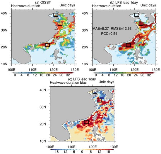
Figure 8.
Duration of the MHW event as recorded in the OISST (a) and the 1-day lead LFS forecast (b), along with the difference between the two (c). The MAE, RMSE, and PCC of the MHW event between the OISST and LFS are shown in (b). Units: days.
The bias in the 1-day-lead-forecasted duration time of the MHW event is further analyzed. Three regions with significant biases (2° × 2° black boxes in Figure 8) are compared with the observations to assess the regional differences. The regionally averaged SST, the MHW threshold from the OISST, and the 1-day lead forecast are presented in Figure 9. In Region 1 (Bohai Sea, Figure 9a), the forecasted duration of the MHW event is less than five days, which is a failure in forecasting the event by LFS. The main reason for the failure is the colder forecasted SST (blue curve in Figure 9a), which only reaches the MHW threshold from 27 September to 1 October. As a result, the forecasted duration of the MHW event in the Bohai Sea has a large bias during October 2021. In Region 2 (Yellow Sea, Figure 9b), the forecasted duration of the MHW event is longer than the observed value. This is because the forecasted SST (blue curve in Figure 9b) is always warmer than the observed SST (black curve in Figure 9b) during the later stage of the event. For instance, although the observed SST is colder than the threshold around 20 October, the predicted SST is still warmer than the threshold, leading to the continuous occurrence of the MHW event (represented by a longer duration) in LFS.
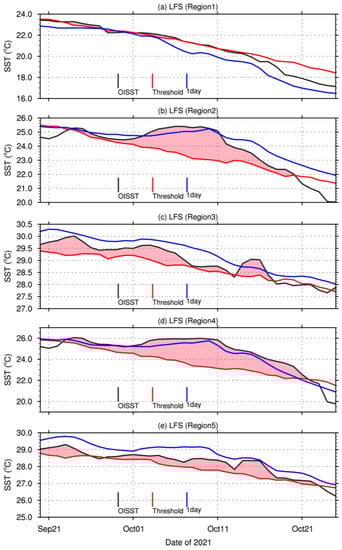
Figure 9.
Time series of observed and forecasted SST and the MHW threshold in five representative regions. (a–e) The time series of area-weight mean SST (OISST, black curves), the threshold of the MHW (MHW, red curves), and the 1-day-lead-forecasted SST (LFS, blue curves) in five representative regions, respectively. The five regions are Region 1 (120° E to 122° E, 38° N to 40° N), Region 2 (122° E to 124° E, 32.8° N to 34.8° N), Region 3 (116° E to 118° E, 20.2° N to 22.2° N), Region 4 (121° E to 123° E, 32° N to 34° N), and Region 5 (118.2° E to 120.2° E, 22.2° N to 24.2° N). The first three regions are marked as black boxes in Figure 8, and the last two are marked as black boxes in Figure 10.
In Region 3 (the northern part of the South China Sea, Figure 9c), the forecasted SST is warmer than the OISST throughout the period. The warm bias peaks around 13 October, when the observed SST starts to be colder than the MHW threshold, indicating the end of the MHW event. However, the 1-day-lead-predicted SST is still warmer than the observations and the MHW threshold, leading to a longer duration bias in LFS. Thus, the warmer 1-day-lead-predicted SST in the northern part of the South China Sea causes a longer duration during extinction.
The influence of the forecast lead time on the duration of the MHW event is also examined based on the three regions. The forecasted SST becomes colder with increasing forecast lead time, causing the forecasted duration of the MHW event to shorten accordingly.
3.3. Intensity of the MHW Event
The results of the intensity of the MHW event indicate that the MHW event is most extreme in the southern Yellow Sea, particularly in its near-shore region, with maximum intensity values reaching up to 3 °C (Figure 10a). Conversely, the intensity of the MHW event in the Bohai Sea and the northern part of the South China Sea is comparatively weaker and falls below 1 °C. The spatial distributions of both intensity and duration reveal that while the MHW event in the southern part of the Yellow Sea is characterized by long duration and strong intensity, the southern part of the East China Sea and the northern part of the South China Sea show weaker intensity despite their longer duration.
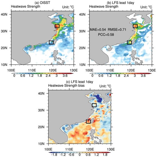
Figure 10.
The intensity of the MHW event from the OISST (a), the 1-day lead forecast from LFS (b), and the difference (c). The MAE, RMSE, and PCC of the intensity of the MHW event between the OISST and LFS are indicated in (b). Unit: °C.
The results of the 1-day lead forecast indicate close agreement with the observations regarding the intensity of the MHW event. The high-intensity MHW event continues to be concentrated in the southern part of the Yellow Sea (Figure 10b). The correlation coefficient between the observations (OISST) and the 1-day lead forecast (LFS) is 0.58, indicating a strong spatial pattern similarity. However, there are negative biases in the forecast intensity north of 30° N and positive biases south of 30° N (Figure 10c). In addition, the forecast intensity weakens with increasing forecast lead time. The absolute intensity error of the 6-day lead forecast is 0.62 °C, and the spatial correlation coefficient decreases to 0.48. The absolute error of the 11-day lead forecast reaches 0.81 °C, and the spatial correlation coefficient drops further to 0.18.
To examine the cause of the large biases in the 1-day lead forecast in the regions identified in Figure 10, we present the regional average SST time series for these areas in Figure 9d,e. Our analysis indicates that the 1-day-lead-forecasted SST is lower than the observed value throughout the MHW event in Region 4, resulting in a weaker intensity. In contrast, in Region 5, off the southwest corner of Taiwan Island, the predicted warm SST biases lead to a stronger MHW intensity throughout the MHW event (Figure 9e).
3.4. Causes of the Biases in SST
The results of the SST budget analysis indicate that both ocean dynamics and net heat flux influence changes in SST. Figure 11 shows the relative changes in SST around China on 6 October compared with 5 October, as well as the changes in SST resulting from the ocean dynamics and surface heat flux terms. As shown in Figure 11a, there is an overall increase in SST across the China Sea, particularly in the Yellow Sea and the East China Sea, except for the Bohai Sea. It is evident that the change in SST is predominantly driven by shortwave radiation (Figure 11d), latent heat (Figure 11e), and ocean dynamics (Figure 11f). These three terms are several-times greater in magnitude than the change in SST caused by sensible heat (Figure 11b) and longwave radiation (Figure 11c). In a similar vein, Kuroda et al. (2021) [38] also identified atmospheric conditions as the primary driver of marine heatwaves. Additionally, Pinault et al. (2022) [39] found that SST anomalies can be non-local. To gain a better understanding of the origin of the forecast bias, we analyze the influence of shortwave radiation, latent heat, and ocean dynamics in the five critical regions.
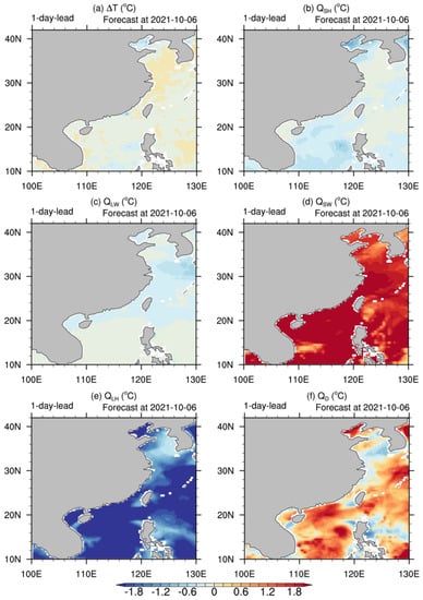
Figure 11.
Heat budget of the relative changes of 1-day-lead-forecasted SST around China. (a) The relative change in 1-day-lead-forecasted SST on 6 October compared with 5 October. (b–f) The relative change in SST on 6 October compared with 5 October caused by the 1-day-lead-forecasted sensible heat, longwave radiation, shortwave radiation, latent heat, and ocean dynamics terms, respectively (unit: °C).
The time evolution of the mean shortwave radiation and latent heat in the five key regions is presented to determine the source of the forecast bias (Figure 12). For Region 1 (located in the Bohai Sea), the 1-day-lead-forecasted shortwave radiation is relatively in line with the ERA5 data during the development and mature period of the MHW event (from 3 October to 11 October), except for 10 October, when the predicted shortwave radiation exceeds that of ERA5 by a maximum difference of around 80 W m−2 (Figure 12a). However, the predicted latent heat is significantly larger than the ERA5 reference, reaching a difference of 300 W m−2, which is greater than the difference in the shortwave radiation. The SST change due to the ocean dynamics term remains close to 0 °C between 3 October and 11 October. A comparison of these three terms reveals that the predicted MHW event’s short duration and weak intensity in the Bohai Sea are primarily driven by the strong predicted latent heat.
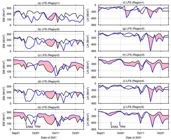
Figure 12.
Evolution of the area–weighted mean shortwave radiation (SW, left panels) in the five study regions. (a–e) Time evolutions of the area–weighted mean shortwave radiation in Region 1 (120° E to 122° E, 38° N to 40° N), Region 2 (122° E to 124° E, 32.8° N to 34.8° N), Region 3 (116° E to 118° E, 20.2° N to 22.2° N), Region 4 (121° E to 123° E, 32° N to 34° N), and Region 5 (118.2° E to 120.2° E, 22.2° N to 24.2° N), respectively, based on ERA5 reanalysis data (black) and the 1-day lead forecast (blue). (f–j) The same as in (a–e), but for latent heat. Units: W m−2.
For Regions 2 and 4 in the Yellow Sea, the 1-day lead forecast of the MHW event duration is longer than the observed value. This discrepancy is primarily due to the warmer SST predicted at the beginning of the event’s extinction period (about 20 October). An analysis of the forecasted shortwave radiation and latent heat in the decay and extinction periods, compared with the ERA5 data (Figure 12), reveals that the forecasted shortwave radiation is stronger than the reference (ERA5) value after 20 October, whereas the deviation in the forecasted latent heat gradually decreases. The increased shortwave radiation in the extinction period causes the predicted SST to be warmer, leading to a longer duration. However, the intensity of the predicted MHW event is weaker than the reference, despite the stronger forecasted shortwave radiation and latent heat during the development and mature periods (Figure 12d,i). The maximum difference in shortwave radiation is about 150 W m−2, and the corresponding latent heat shows a negative deviation of about 100 W m−2. The ocean dynamics term (Figure 13b,d) is inferred to be the reason for the colder predicted SST and weaker MHW intensity.
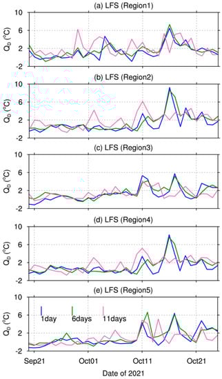
Figure 13.
(a–e) Time evolution of the relative change in the area-weighted mean SST on 6 October compared with 5 October caused by the 1-day-lead-forecasted ocean dynamics term in Region 1 (120° E to 122° E, 38° N to 40° N), Region 2 (122° E to 124° E, 32.8° N to 34.8° N), Region 3 (116° E to 118° E, 20.2° N to 22.2° N), Region 4 (121° E to 123° E, 32° N to 34° N), and Region 5 (118.2° E to 120.2° E, 22.2° N to 24.2° N), respectively, for the 1-day lead forecast (blue), 6-day lead forecast (green), and 11-day lead forecast (pink). Unit: °C.
For Region 3, in the northern part of the South China Sea, the duration of the 1-day lead forecast extends beyond that of the observed SST (OISST), largely due to the warmer predicted SST in the decay period (Figure 9c). As seen in Figure 12h, the predicted latent heat exhibits a consistent positive deviation compared with the reference throughout the entire period. In contrast, the forecasted shortwave radiation (Figure 12c) begins to exceed the reference value around 20 October, which corresponds with the time when the SST is predicted to start increasing. Hence, it can be concluded that the extended forecast duration in the northern part of the South China Sea is primarily driven by the stronger predicted shortwave radiation during the decay period of the MHW event.
In Region 5 of the northern South China Sea, the 1-day lead forecast of the MHW event intensity is higher than the observations. As depicted in the Region 5 SST time series (Figure 9e), the increased intensity of the MHW event is a result of the warmer predicted SST values, especially during the development phase of the event. A comparison of the predicted shortwave radiation and latent heat (Figure 12e,j) reveals that the predicted shortwave radiation has a substantial positive deviation during the development phase, contributing to the stronger intensity. Therefore, by combining the results of Region 3 and Region 5 in the northern South China Sea, it can be concluded that the longer duration and increased intensity of the predicted MHW event in the north of the South China Sea are mainly caused by the stronger predicted shortwave radiation.
The results show a trend of decreasing duration and weakened intensity of the predicted MHW event with increasing forecast lead time. The analysis of the primary factors influencing the MHW event shows that the forecasted shortwave radiation consistently decreases with a longer forecast lead time. Conversely, the forecasted latent heat flux and ocean dynamics term (Figure 13) do not show a clear pattern of change with increasing forecast lead time. The reduction in forecasted shortwave radiation decreases SST warming and may contribute to the decline in or disappearance of the MHW event. This trend explains the shortened duration and weakened intensity of the predicted MHW event as the forecast lead time increases.
4. Summary and Discussion
This study assesses the accuracy of a high-resolution global ocean forecast system (LFS) in predicting MHW events around China during September–October 2021, using the definition of MHW events modified from Hobday et al. (2016). The results indicate that LFS can predict the MHW event around China with a 1-day lead time. The system can accurately predict the occurrence of the MHW event in up to 79% of the area observed (Figure 4), with an accuracy rate of around 60% throughout the MHW event (averaged Ratio in Figure 4). In addition, the system demonstrates better accuracy during the initial and decay periods compared with other event stages.
Regarding the duration of the MHW event, the results of the 1-day lead forecast by LFS demonstrate a strong agreement with the observations. The southern part of the Yellow Sea and the northern part of the Southern China Sea show longer durations, surpassing 30 days, which is slightly extended compared with the observed data. A detailed analysis of two distinct regions within the Yellow Sea and the Southern China Sea reveals that the predicted stronger shortwave radiation flux primarily drives the prolonged forecast duration during the decay period of the MHW event.
Regarding the intensity of the MHW event, the 1-day lead forecast by LFS shows good agreement with the observations, with an RMSE of only 0.71 °C. The northern part of the Yellow Sea shows a relatively small deviation, while the southern part exhibits a substantial deviation. Analysis of the time series of five selected regions reveals that the weak intensity in the northern Yellow Sea is primarily attributed to the deviation in the ocean dynamics term, as deviations in the predicted shortwave radiation and latent heat tend to enhance the intensity.
In addition, as the forecast lead time increases, the spatial distribution bias of the predicted duration increases, and the predicted duration decreases. This reduction in predicted duration is primarily due to the decline in the predicted shortwave radiation with increasing forecast lead time. Similarly, the weakening of the predicted intensity with increasing forecast lead time can also be attributed to the decline in the predicted shortwave radiation.
In conclusion, this study evaluated the performance of a high-resolution global ocean forecast system (LFS) in predicting an extreme warm water event (MHW) around China during September–October 2021. The results indicate that LFS has a good forecasting ability for the MHW event with a lead time of one day, with a high degree of accuracy regarding occurrence range, duration, and intensity. However, there are some areas of deviation between the forecast and observations, particularly in the Bohai Sea and the South China Sea, where improvements in the latent heat and shortwave radiation fluxes in the forcing field of the forecast system could enhance the forecasting performance. In the southern Yellow Sea and northern East China Sea, an improved simulation of ocean dynamics heat transport is necessary to improve the future forecasting ability of MHW events.
Author Contributions
Conceptualization, J.L. and P.L.; methodology, validation, formal analysis, and writing—original draft preparation, Y.L.; investigation, Y.L. and W.Z.; software, Z.Y. and J.C.; writing—review and editing, Y.L., J.L., H.L. and P.L.; supervision, H.L. All authors have read and agreed to the published version of the manuscript.
Funding
This research was funded by the National Key R&D Program for Developing Basic Sciences (2022YFC3104802), the Special Funds for Creative Research (2022C61540), State Key Laboratory of Cryospheric Science, Northwest Institute of Eco-Environment and Resources, Chinese Academy Sciences (Grant Number: SKLCS-OP-2021-08), the National Natural Science Foundation of China (Grant 42106020), and the Key Program of the National Natural Science Foundation of China (Grants 41931183 and 41931182).
Institutional Review Board Statement
Not applicable.
Informed Consent Statement
Not applicable.
Data Availability Statement
The data in this study are available on request from the corresponding author.
Acknowledgments
The authors acknowledge the technical support from the National Key Scientific and Technological Infrastructure project “Earth System Science Numerical Simulator Facility” (EarthLab). We are grateful to anonymous referees and the editor who provided valuable comments improving the manuscript.
Conflicts of Interest
The authors declare no conflict of interest.
References
- Oliver, E.C.; Donat, M.G.; Burrows, M.T.; Moore, P.J.; Smale, D.A.; Alexander, L.V.; Benthuysen, J.A.; Feng, M.; Sen Gupta, A.; Hobday, A.J.; et al. Longer and more frequent marine heatwaves over the past century. Nat. Commun. 2018, 9, 1324. [Google Scholar] [CrossRef] [PubMed]
- Holbrook, N.J.; Scannell, H.A.; Sen Gupta, A.; Benthuysen, J.A.; Feng, M.; Oliver, E.C.; Alexander, L.V.; Burrows, M.T.; Donat, M.G.; Hobday, A.J.; et al. A global assessment of marine heatwaves and their drivers. Nat. Commun. 2019, 10, 2624. [Google Scholar] [CrossRef] [PubMed]
- Miao, Y.Q.; Xu, H.M.; Liu, J.W. Variation of summer marine heatwaves in the Northwest Pacific and associated air-sea interaction. J. Trop. Oceanogr. 2021, 40, 31–43. [Google Scholar]
- Wernberg, T.; Smale, D.A.; Tuya, F.; Thomsen, M.S.; Langlois, T.J.; De Bettignies, T.; Bennett, S.; Rousseaux, C.S. An extreme climatic event alters marine ecosystem structure in a global biodiversity hotspot. Nat. Clim. Chang. 2013, 3, 78–82. [Google Scholar] [CrossRef]
- Mills, K.E.; Pershing, A.J.; Brown, C.J.; Chen, Y.; Chiang, F.S.; Holland, D.S.; Lehuta, S.; Nye, J.A.; Sun, J.C.; Thomas, A.C.; et al. Fisheries management in a changing climate: Lessons from the 2012 ocean heat wave in the Northwest Atlantic. Oceanography 2013, 26, 191–195. [Google Scholar] [CrossRef]
- Oliver, E.C.; Benthuysen, J.A.; Bindoff, N.L.; Hobday, A.J.; Holbrook, N.J.; Mundy, C.N.; Perkins-Kirkpatrick, S.E. The unprecedented 2015/16 Tasman Sea marine heatwave. Nat. Commun. 2017, 8, 16101. [Google Scholar] [CrossRef]
- Smale, D.A.; Wernberg, T.; Oliver, E.C.; Thomsen, M.; Harvey, B.P.; Straub, S.C.; Burrows, M.T.; Alexander, L.V.; Benthuysen, J.A.; Donat, M.G.; et al. Marine heatwaves threaten global biodiversity and the provision of ecosystem services. Nat. Clim. Chang. 2019, 9, 306–312. [Google Scholar] [CrossRef]
- Benthuysen, J.A.; Oliver, E.C.; Chen, K.; Wernberg, T. Advances in understanding marine heatwaves and their impacts. Front. Mar. Sci. 2020, 7, 147. [Google Scholar] [CrossRef]
- Qin, H.; Kawamura, H.; Kawai, Y. Detection of hot event in the equatorial Indo-Pacific warm pool using advanced satellite sea surface temperature, solar radiation, and wind speed. J. Geophys. Res. Ocean. 2007, 112, C07015. [Google Scholar] [CrossRef]
- Sorte, C.J.; Fuller, A.; Bracken, M.E. Impacts of a simulated heat wave on composition of a marine community. Oikos 2010, 119, 1909–1918. [Google Scholar] [CrossRef]
- Wernberg, T.; Smale, D.A.; Thomsen, M.S. A decade of climate change experiments on marine organisms: Procedures, patterns and problems. Glob. Chang. Biol. 2012, 18, 1491–1498. [Google Scholar] [CrossRef]
- Hobday, A.J.; Alexander, L.V.; Perkins, S.E.; Smale, D.A.; Straub, S.C.; Oliver, E.C.; Benthuysen, J.A.; Burrows, M.T.; Donat, M.G.; Feng, M.; et al. A hierarchical approach to defining marine heatwaves. Prog. Oceanogr. 2016, 141, 227–238. [Google Scholar] [CrossRef]
- Frölicher, T.L.; Fischer, E.M.; Gruber, N. Marine heatwaves under global warming. Nature 2018, 560, 360–364. [Google Scholar] [CrossRef] [PubMed]
- Bond, N.A.; Cronin, M.F.; Freeland, H.; Mantua, N. Causes and impacts of the 2014 warm anomaly in the NE Pacific. Geophys. Res. Lett. 2015, 42, 3414–3420. [Google Scholar] [CrossRef]
- Capotondi, A.; Jacox, M.; Bowler, C.; Kavanaugh, M.; Lehodey, P.; Barrie, D.; Brodie, S.; Chaffron, S.; Cheng, W.; Dias, D.F.; et al. Observational needs supporting marine ecosystems modeling and forecasting: From the global ocean to regional and coastal systems. Front. Mar. Sci. 2019, 6, 623. [Google Scholar] [CrossRef]
- Park, H.S.; Lee, S.; Son, S.W.; Feldstein, S.B.; Kosaka, Y. The impact of poleward moisture and sensible heat flux on Arctic winter sea ice variability. J. Clim. 2015, 28, 5030–5040. [Google Scholar] [CrossRef]
- Schmeisser, L.; Bond, N.A.; Siedlecki, S.A.; Ackerman, T.P. The role of clouds and surface heat fluxes in the maintenance of the 2013–2016 Northeast Pacific marine heatwave. J. Geophys. Res. Atmos. 2019, 124, 10772–10783. [Google Scholar] [CrossRef]
- Di Lorenzo, E.; Mantua, N. Multi-year persistence of the 2014/15 North Pacific marine heatwave. Nat. Clim. Chang. 2016, 6, 1042–1047. [Google Scholar] [CrossRef]
- Zhi, H.; Zhang, R.H.; Lin, P.; Shi, S. Effects of salinity variability on recent El Niño events. Atmosphere 2019, 10, 475. [Google Scholar] [CrossRef]
- Yan, Y.; Chai, F.; Xue, H.; Wang, G. Record-breaking sea surface temperatures in the Yellow and East China Seas. J. Geophys. Res. Ocean. 2020, 125, e2019JC015883. [Google Scholar] [CrossRef]
- Behrens, E.; Fernandez, D.; Sutton, P. Meridional oceanic heat transport influences marine heatwaves in the Tasman Sea on interannual to decadal timescales. Front. Mar. Sci. 2019, 6, 228. [Google Scholar] [CrossRef]
- Jacox, M.G.; Alexander, M.A.; Amaya, D.; Becker, E.; Bograd, S.J.; Brodie, S.; Hazen, E.L.; Pozo Buil, M.; Tommasi, D. Global seasonal forecasts of marine heatwaves. Nature 2022, 604, 486–490. [Google Scholar] [CrossRef] [PubMed]
- Liu, H.; Lin, P.; Zheng, W.; Luan, Y.; Ma, J.; Ding, M.; Mo, H.; Wan, L.; Ling, T. A global eddy-resolving ocean forecast system in China–LICOM Forecast System (LFS). J. Oper. Oceanogr. 2023, 16, 15–27. [Google Scholar] [CrossRef]
- Chassignet, E.P.; Yeager, S.G.; Fox-Kemper, B.; Bozec, A.; Castruccio, F.; Danabasoglu, G.; Horvat, C.; Kim, W.M.; Koldunov, N.; Li, Y.; et al. Impact of horizontal resolution on global ocean–sea ice model simulations based on the experimental protocols of the Ocean Model Intercomparison Project phase 2 (OMIP-2). Geosci. Model Dev. 2020, 13, 4595–4637. [Google Scholar] [CrossRef]
- Li, Y.; Liu, H.; Ding, M.; Lin, P.; Yu, Z.; Yu, Y.; Meng, Y.; Li, Y.; Jian, X.; Jiang, J.; et al. Eddy-resolving simulation of CAS-LICOM3 for Phase 2 of the ocean model intercomparison project. Adv. Atmos. Sci. 2020, 37, 1067–1080. [Google Scholar] [CrossRef]
- Lin, P.; Yu, Z.; Liu, H.; Yu, Y.; Li, Y.; Jiang, J.; Ma, J. LICOM model datasets for the CMIP6 ocean model intercomparison project. Adv. Atmos. Sci. 2020, 37, 239–249. [Google Scholar] [CrossRef]
- Tsujino, H.; Urakawa, L.S.; Griffies, S.M.; Danabasoglu, G.; Adcroft, A.J.; Amaral, A.E.; Arsouze, T.; Bentsen, M.; Bernardello, R.; Böning, C.W.; et al. Evaluation of global ocean–sea-ice model simulations based on the experimental protocols of the Ocean Model Intercomparison Project phase 2 (OMIP-2). Geosci. Model Dev. 2020, 13, 3643–3708. [Google Scholar] [CrossRef]
- Wang, P.; Jiang, J.; Lin, P.; Ding, M.; Wei, J.; Zhang, F.; Zhao, L.; Li, Y.; Yu, Z.; Zheng, W.; et al. The GPU version of LASG/IAP Climate System Ocean Model version 3 (LICOM3) under the heterogeneous-compute interface for portability (HIP) framework and its large-scale application. Geosci. Model Dev. 2021, 14, 2781–2799. [Google Scholar] [CrossRef]
- Zheng, W.; Lin, P.; Liu, H.; Luan, Y.; Ma, J.; Mo, H.; Liu, J. An assessment of the LICOM Forecast System (LFS) under the IVTT class4 framework. Front. Mar. Sci. 2023, 10, 696. [Google Scholar]
- Reynolds, R.W.; Smith, T.M.; Liu, C.; Chelton, D.B.; Casey, K.S.; Schlax, M.G. Daily high-resolution-blended analyses for sea surface temperature. J. Clim. 2007, 20, 5473–5496. [Google Scholar] [CrossRef]
- Banzon, V.; Smith, T.M.; Chin, T.M.; Liu, C.; Hankins, W. A long-term record of blended satellite and in situ sea-surface temperature for climate monitoring, modeling, and environmental studies. Earth Syst. Sci. Data 2016, 8, 165–176. [Google Scholar] [CrossRef]
- Huang, B.; Liu, C.; Banzon, V.; Freeman, E.; Graham, G.; Hankins, B.; Smith, T.; Zhang, H.-M. Improvements of the daily optimum interpolation sea surface temperature (DOISST) version 2.1. J. Clim. 2021, 34, 2923–2939. [Google Scholar] [CrossRef]
- Hersbach, H.; Bell, B.; Berrisford, P.; Biavati, G.; Horányi, A.; Muñoz Sabater, J.; Nicolas, J.; Peubey, C.; Radu, R.; Rozum, I.; et al. ERA5 Hourly Data on Single Levels from 1940 to Present. Copernicus Climate Change Service (C3S) Climate Data Store (CDS). 2023. Available online: https://cds.climate.copernicus.eu/cdsapp#!/dataset/reanalysis-era5-single-levels?tab=overview (accessed on 26 March 2023).
- Waliser, D.E. Formation and limiting mechanisms for very high sea surface temperature: Linking the dynamics and the thermodynamics. J. Clim. 1996, 9, 161–188. [Google Scholar] [CrossRef]
- Mandal, R.; Joseph, S.; Sahai, A.K.; Phani, R.; Dey, A.; Chattopadhyay, R.; Pattanaik, D.R. Real time extended range prediction of heat waves over India. Sci. Rep. 2019, 9, 1–11. [Google Scholar] [CrossRef] [PubMed]
- Ferro, C.A.; Stephenson, D.B. Extremal dependence indices: Improved verification measures for deterministic forecasts of rare binary events. Weather. Forecast. 2011, 26, 699–713. [Google Scholar] [CrossRef]
- Stevenson, J.W.; Niiler, P.P. Upper ocean heat budget during the Hawaii-to-Tahiti shuttle experiment. J. Phys. Oceanogr. 1983, 13, 1894–1907. [Google Scholar] [CrossRef]
- Pinault, J.-L. Morlet Cross-Wavelet Analysis of Climatic State Variables Expressed as a Function of Latitude, Longitude, and Time: New Light on Extreme Events. Math. Comput. Appl. 2022, 27, 50. [Google Scholar] [CrossRef]
- Kuroda, H.; Setou, T. Extensive Marine Heatwaves at the Sea Surface in the Northwestern Pacific Ocean in Summer 2021. Remote Sens. 2021, 13, 3989. [Google Scholar] [CrossRef]


Disclaimer/Publisher’s Note: The statements, opinions and data contained in all publications are solely those of the individual author(s) and contributor(s) and not of MDPI and/or the editor(s). MDPI and/or the editor(s) disclaim responsibility for any injury to people or property resulting from any ideas, methods, instructions or products referred to in the content. |
© 2023 by the authors. Licensee MDPI, Basel, Switzerland. This article is an open access article distributed under the terms and conditions of the Creative Commons Attribution (CC BY) license (https://creativecommons.org/licenses/by/4.0/).