Article

A Prediction Method of Ship Motion Based on LSTM Neural Network with Variable Step-Variable Sampling Frequency Characteristics

Logistics Engineering College, Shanghai Maritime University, Shanghai 201306, China
*
Author to whom correspondence should be addressed.
J. Mar. Sci. Eng. 2023, 11(5), 919; https://doi.org/10.3390/jmse11050919
Submission received: 31 March 2023 / Revised: 20 April 2023 / Accepted: 24 April 2023 / Published: 25 April 2023
(This article belongs to the Section Ocean Engineering)

Abstract

:
In active heave compensation, in order to realize the smooth control of the heave compensation platform, it is necessary to use the ship motion measurement system to accurately obtain the ship displacement signal, invert the ship displacement signal, and then control the expansion and contraction of the electric cylinder so that the compensation platform remains horizontal. The ship displacement measurement system generally adopts the second integral of the acceleration sensor to obtain the ship displacement signal. During the acquisition process of the ship displacement signal, the quadratic integration process of the acceleration, and the communication process of the output control command, there is a processing lag which makes the error accumulate, resulting in a delay in the measurement of the ship motion. In order to collect the ship motion more accurately and control the heave compensation platform more precisely, this paper proposes a ship motion prediction method based on a variable step-variable sampling frequency characteristic LSTM (Long Short-Term Memory) neural network. First, we use the autocorrelation function algorithm to calculate the inherent delay of the lag in the process of signal acquisition by the measurement system. Secondly, the LSTM neural network is used to predict the inherent delay step of the lagging ship displacement signal. During the prediction process, it is found that the difference in the sampling frequency of the displacement signal will lead to a change in the step of the inherent delay—experiment in the laboratory to verify. By controlling the motion platform to simulate the motion of the ship and using the ship motion measurement system and the laser sensor system to measure the displacement signal of the motion platform synchronously, it is verified that the ship motion measurement system does have an inherent delay. Thirdly, on a sailing ship, ship displacement signals are collected by setting multiple sets of ship motion measurement systems. Finally, multiple sets of sampling frequency and multiple steps are set, and the ship motion is predicted based on the variable step-variable sampling frequency LSTM neural network. It is verified that the prediction accuracy is related to the sampling frequency of the signal collector and the prediction step of the LSTM neural network, which improves the prediction accuracy of the model and the timeliness of ship motion acquisition.

1. Introduction

Heave compensation technologies are currently mainly divided into two categories: passive heave compensation and active heave compensation [1]. Passive heave compensation generally belongs to an open-loop system, and the system input is the ship motion while the output is a reduced amplitude motion of the attached object. At the same time, passive wave compensation does not require additional energy input, and mainly relies on elastic elements, such as dampers, to reduce the vibration amplitude of the ship. A paper by Hatleskog and Dunnigan (2006) concludes by stating that a passive compensator can be no more than roughly 80% effective, which the authors support through field experience and simulation [2]. Compared with passive heave compensation, active heave compensation is generally a closed-loop system that requires an external energy input. In the active heave compensation system, it is first necessary to measure the ship motion signal; secondly, the displacement command is deciphered according to the ship motion signal to control the load against the heave motion. So, if a ship heaves upward, the controller commands the load to move downward that same amount [3].
Active heave compensation systems currently use inertial measurement units and gyroscopes to measure ship motion, and the processing time of the inertial units will lead to the accumulation of time errors in the measurement process. At the same time, when controlling the drive unit, the problem of inherent delay will also be introduced due to slow communication. Therefore, how to eliminate the time delay generated by the motion measurement module in the active heave compensation system is still one of the difficult problems in engineering testing [4]. A system by Kyllingstad (2012), for example, applied transfer function filters to correct for time/phase lag in their overall system [5]. Alternatively, Kuchler et al. (2011) used heave-prediction algorithms to predict vessel heave motion based on previous measurements and then applied control action based on these predicted motions [6]. Now, as more advanced algorithms and better sensors are included in AHC systems, control quality improves; however, there are disadvantages to the inclusion of more advanced components [7,8,9,10,11]. In order to eliminate the effect of the delay inherent in active heave compensation, Jorg Neupert proposed a heave compensation system based on heave motion prediction and an inversion-based control strategy, and then a prediction algorithm is presented and evaluated with simulation and measurement results [12]. Woodacre J K used the MPC controller to track a variety of test cases and references while outperforming the tuned PID controller for all experiments [13]. Shi B presents an active heave prediction modeling method based on a support vector machine for regression (SVR) using the particle swarm algorithm (KPSO), improved by Kalman filter, to train the parameters of the SVR and predict control [14]. At the same time, with the neural network algorithm proposed, its prediction function is more and more applied to the prediction of active wave compensation [15,16,17,18]. For example, neural networks used for time series prediction, such as LSTM (Long Short-Term Memory), have also been gradually applied to ship motion prediction in recent years [19,20,21,22,23,24]. Su Y proposed a real-time ship vertical acceleration prediction algorithm based on the long short-term memory (LSTM) and gated recurrent units (GRU) models of a recurrent neural network. The prediction results revealed that the proposed algorithm could accurately predict the acceleration time history data of the large-scale ship model, and the root mean square error between the predicted and real values was no greater than 0.1 [25]. Aiming at the problem of the low accuracy of ship roll angle prediction by traditional prediction algorithms and the single neural network model, Wang Y proposed a ship roll angle prediction method based on a bidirectional long short-term memory network (Bi-LSTM) and a temporal pattern attention mechanism (TPA) combined deep learning model; temporal pattern attention mechanism extracts the time patterns from the deep features of a bidirectional long short-term memory network output state that are beneficial to ship roll angle prediction and ignores other features that contribute less to the prediction [26]. For the prediction of ship heave motion, the prediction time step is particularly important, so calculating the delay in the ship motion acquisition system is also a top priority [27,28,29]. Hu T developed an adaptive time delay compensation algorithm based on thorough analysis of the integrated information transmission platform and the composition and characteristics of the time delay in channel, during which forward and reverse transmission channels have been developed properly [30]. The neural network algorithm is gradually widely used in the field of ship motion signal prediction [31,32]. Kaklis D examines how a predictive FOC scheme can be coupled with WR optimization algorithms in order to reduce the vessel’s FOC, emissions, and the overall cost of a voyage [33]. Kaklis D presents a holistic approach to continuously monitor and estimate the emissions of a vessel as well as to assess and improve the efficiency of scrubbers [34]. Kaklis D presents an online learning framework that employs a custom encoding–decoding Neural Network scheme and real-time data from various on-board sensors to appropriately update FOC estimation models [35].
In this paper, in order to further improve the accuracy of active heave compensation and eliminate the time delay problem in the active heave compensation control system, a prediction method of ship motion based on LSTM neural network with variable step-variable sampling frequency characteristics is proposed. First of all, in the process of ship motion measurement, there are problems of integral calculation and slow communication between the hardware modules of the measurement system, resulting in a time delay between the measured ship motion and the real motion of the ship. Secondly, according to the autocorrelation function algorithm, the cross-correlation analysis of the measured ship motion signal and the real motion signal is used to calculate the inherent time of the measurement system delay. Then, the sampling frequency of the ship motion signal is changed to determine the time step that needs to be predicted through the obtained inherent time. Next, we build the LSTM neural network model with variable step-variable sampling frequency characteristics. At the same time, a data set is built according to the low-frequency time characteristics of the ship motion, and the model weights are trained. Finally, the ship motion signal is predicted using the trained neural network model, eliminating the inherent delay in active heave compensation measurement systems.
In order to verify the prediction effect of the proposed LSTM neural network with variable step-variable sampling frequency characteristics, we conducted experimental verification. The existing heave motion platform in the laboratory was used to simulate the motion of the ship, and a laser sensor measurement point and a ship motion measurement system were built on the platform. The laser sensor and the ship motion measurement system were used to collect displacement signals at the same time, and the cross-correlation analysis of the two signals was used to solve the inherent delay in the ship motion measurement system. The ship motion signal was predicted by eight groups of LSTM neural networks with variable step-variable sampling frequency characteristics. The experiments proved that the LSTM neural network with variable step-variable sampling frequency characteristics can accurately predict the heave displacement value of the ship, and is more suitable for the prediction of low-frequency motion of the ship.
The main contributions of this paper are summarized as follows:
  • An algorithm to eliminate the inherent time delay in the active heave compensation measurement system was proposed. Using the autocorrelation function, the inherent delay in the measurement system was solved by performing a cross-correlation analysis on the actual motion signal of the ship and the signal collected by the ship measurement system. According to the obtained inherent delay, the LSTM neural network with variable step-variable sampling frequency characteristics was built to predict the ship heave signal.
  • According to the obtained inherent delay, a ship motion prediction method based on an LSTM neural network with variable step-variable sampling frequency characteristics was proposed to predict the ship heave signal. The formulation of the training set was improved according to the characteristics of the low-frequency motion of the ship. The training set not only included the short-term period characteristics of the low-frequency ship motion, but also included the long-term characteristics of the ship under the influence of the wave force. It made the predicted waveform signal more suitable for the prediction of ship movement.
The subsequent sections of this manuscript are organized as follows: Section 2 presents the preliminary work. Section 3 describes in detail the solution to the inherent delay of the measurement system and the proposed LSTM neural network with variable step-variable sampling frequency characteristics. Section 4 designs experimental validation for the proposed algorithms. Section 5 presents the conclusion and provides suggestions for future work.

2. Preliminary Work

The time delay generated by the ship motion measurement system is mainly composed of two parts: the calculation time of the inertial sensor unit integration, and the communication time between the signal collector and the host computer. The time delay generated by these two parts is determined by the hardware device properties of the system, so the delay in the ship motion measurement system is an inherent time. In order to eliminate the inherent delay, the inherent delay of the system is obtained by the autocorrelation function algorithm, and the LSTM neural network with variable step-variable sampling frequency characteristics is used to predict the ship motion signal in the inherent delay stage.

2.1. Autocorrelation Function

Under actual sea conditions, the ship motion signal collected through the integral calculation of the inertial sensor unit will inevitably be disturbed by noise, and the signal data may be completely lost in severe cases. The autocorrelation function describes the degree of correlation between a random signal at different times. It can find repetitive information from the ship motion signal and identify the fundamental frequency implied in the harmonic frequency of the signal. Its definition is:
R x , x = E ( x ( t 1 ) , x ( t 2 ) )
For continuous signals, the definition is:
R x , x ( τ ) = + x ( t ) x ( t + τ ) d t
For discrete signals, the definition is:
R x , x ( n ) = n = + x ( m ) x ( m + n )

2.2. LSTM Neural Network

The input and output of many neural networks are independent of each other, such as the BP neural network, convolutional neural network (CNN), etc. However, in the time series prediction of ship heave displacement, the prediction at the later time is related to the data at the previous time. Recurrent Neural Networks (RNN) introduce the concept of “memory”, which allows information to be persisted. The RNN structure diagram is shown in Figure 1.
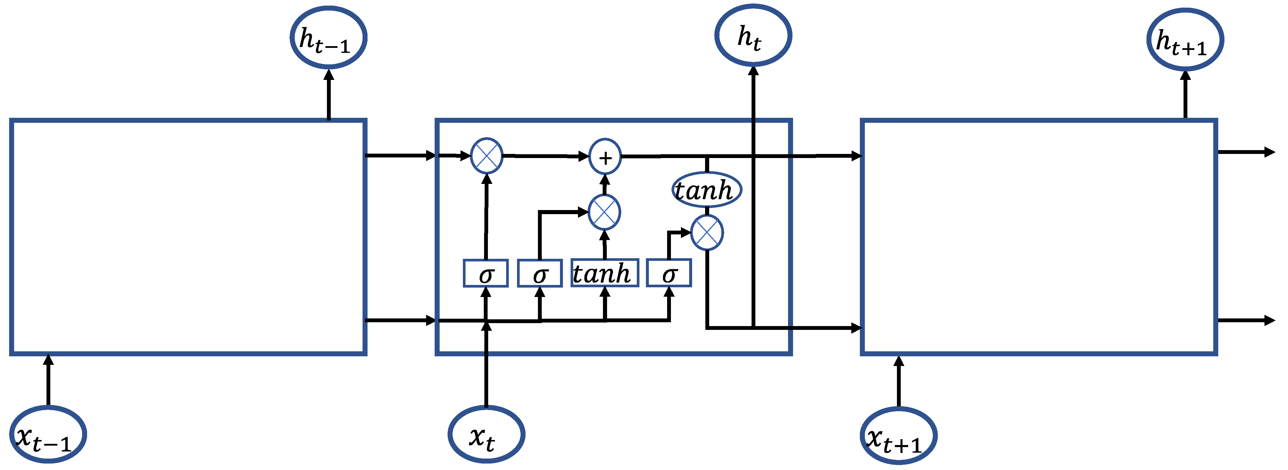
The heave motion of the ship is affected by the wave force, which belongs to the same low-frequency motion as the sea wave. Therefore, short time series training cannot guarantee that the model learns the long-term characteristic knowledge of ship heave motion. However, the RNN does not work well in long-term dependent problems. An RNN will remember all the previous information in the long-term sequence, the newly added input information will reduce the weight ratio of the previous information, and the last retained information may be worthless information. Therefore, when the prediction needs to rely on earlier long-term information, with the continuous increase of the time dimension, it is difficult for an RNN to retain the information at an earlier time and cannot guarantee the accuracy of the ship heave displacement prediction. The long short-term memory network (LSTM) solves the problem of long-term dependence of an RNN very well. LSTM is a special case of RNNs, and an algorithm improved on RNNs. It can filter out useful information and save it, which solves the problem of an RNN gradient disappearance and gradient explosion. The structural situation diagram of the LSTM neural network is shown in Figure 2.
The core part of the LSTM neural network is the cell state of the LSTM unit. The LSTM controls the increase or decrease of information through the “gate” structure, and selectively allows information to pass through, thereby realizing the functions of memory and forgetting. A cell contains an input gate, a forget gate, and an output gate.
Forget gate: The forget gate f t can save the ship movement signal from a long time ago, and determines how much “knowledge” of the unit state at the last moment can be retained to the current moment. It is a sigmoid function whose input is the output of the previous unit h t 1 and the input of this unit x t . The output range is 0~1, which is assigned to the current cell state, and its calculation formula is:
f t = σ ( W f [ h t 1 , x t ] )
Among them, [ h t 1 , x t ] means to connect the current input vector and the output vector at the previous moment to form a vector with a larger dimension, W f is the weight matrix, and σ is the sigmoid function.
Input gate: The input gate i t can prevent unimportant ship motion signals from entering the memory cells at the current moment. It works with the tanh function to control the addition of new ship motion signals. The tanh function generates a candidate C t ˜ , which is multiplied by the sigmoid function to control the addition of new ship displacement signals. Its calculation formula is:
i t = σ ( W i [ h t 1 , x t ] )
C t ˜ = tanh ( W c [ h t 1 , x t ] )
Update the memory unit: update the old cell state C t 1 . Its calculation formula is:
C t = f t C t 1 + i t C t ˜
Output gate: The output gate o t is used to determine the value of the next hidden state, which contains the previous information. First, we use the Sigmoid layer to get an initial part of the output. Then, we use the tanh function to scale the value of C t to [−1, 1]. Then, we multiply the output results obtained by the previous sigmoid layer in turn to obtain the final output h t . Its calculation formula is:
o t = σ ( W o [ h t 1 , x t ] )
h t = o t tanh ( C t )
Activation function:
The function of the Sigmoid function is to map the input to [0, 1], and its function expression is:
s i g m o i d ( x ) = 1 1 + e x
The function of the Tanh function is to map the input to [−1, 1], and its function expression is:
tanh ( x ) = e x + e x e x + e x

3. The Proposed Method

3.1. Solution of Inherent Delay in Ship Motion Measurement System

In order to accurately measure the inherent delay produced by the ship motion measurement system, it is necessary to determine the reference signal first. In this paper, the ship motion signal collected by a high-sensitivity laser sensor is used as the reference signal. The timing signal of the ship displacement collected by the ship motion measurement system is defined as x ( t ) , the timing reference signal collected by the laser sensor is defined as y ( t ) , and the cross-correlation analysis is carried out. Cross-correlation can be considered as a special case of autocorrelation function, which is used to describe the degree of correlation between the values of ship displacement signal x ( t ) and laser reference signal y ( t ) at any two different moments t 1 and t 2 . According to the cross-correlation analysis, it reflects the physical meaning of the similarity of the two displacement signals involved in the operation: when the value of the coordinate variable of the laser reference signal x ( t ) changes in the discrete domain, there will always be a discrete coordinate value n * that makes the reference signal most similar to the echo signal of the ship motion measurement system with delay information. At this time, the value of the autocorrelation function reaches the peak point, and the abscissa n * corresponding to the peak point is the estimated value of the discrete time delay obtained by this method. Its calculation formula is:
R x , y = E ( x ( t 1 ) , y ( t 2 ) )
The calculation formula of discrete time series signal is:
R x , y ( n ) = n = + x ( m ) y ( m + n )
Peak retrieval is performed on the discrete domain for this cross-correlation function. The inherent delay of the ship motion measurement system is obtained as:
n * = τ = arg { max ( R x , y ) }
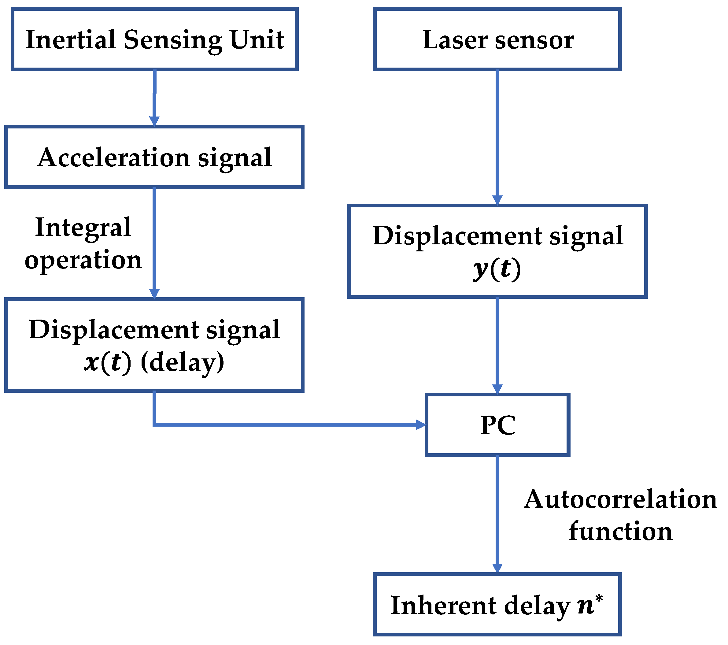
Among them, τ is the inherent delay, arg { · } means to get the independent variable value of the function, and max { · } means to get the maximum value of the function. The structural process for solving the inherent delay is shown in Figure 3.

3.2. LSTM Neural Network with Variable Step-Variable Sampling Frequency Characteristics

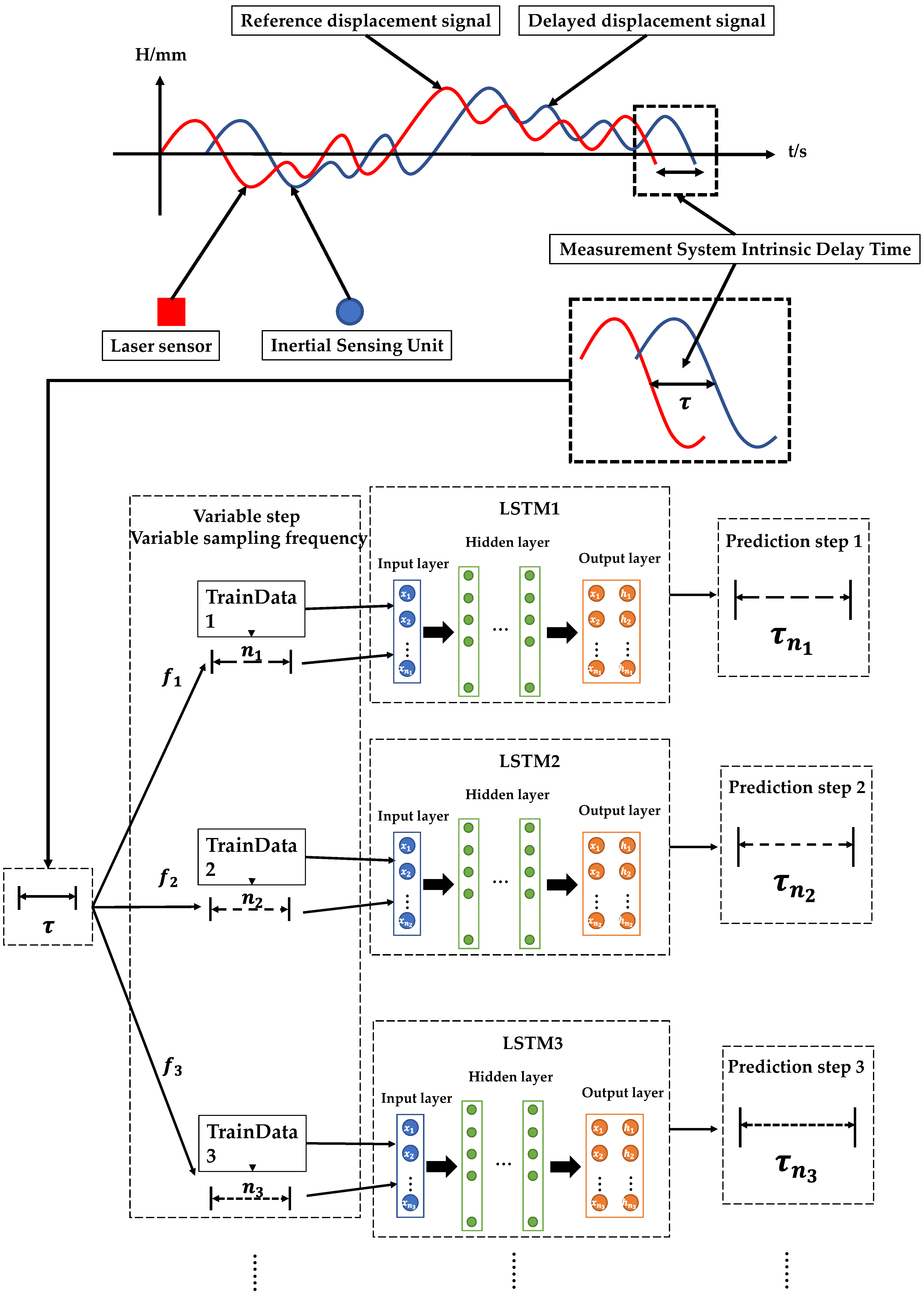
Variable step-variable sampling frequency: In order to predict the inherent delay generated in the heave compensation system, it is necessary to determine the prediction time step of the LSTM neural network. The LSTM neural network prediction time step is related to the prediction accuracy. With a certain inherent delay, the prediction time step is determined by the sampling frequency of the ship heave motion signal. When the sampling frequency of the signal changes, the prediction time step also changes accordingly. The formula for calculating the forecast time step is:
n = τ f s
Among them, n is the prediction time step, τ is the inherent delay obtained by cross-correlation analysis, and f s is the sampling frequency of the ship motion signal.
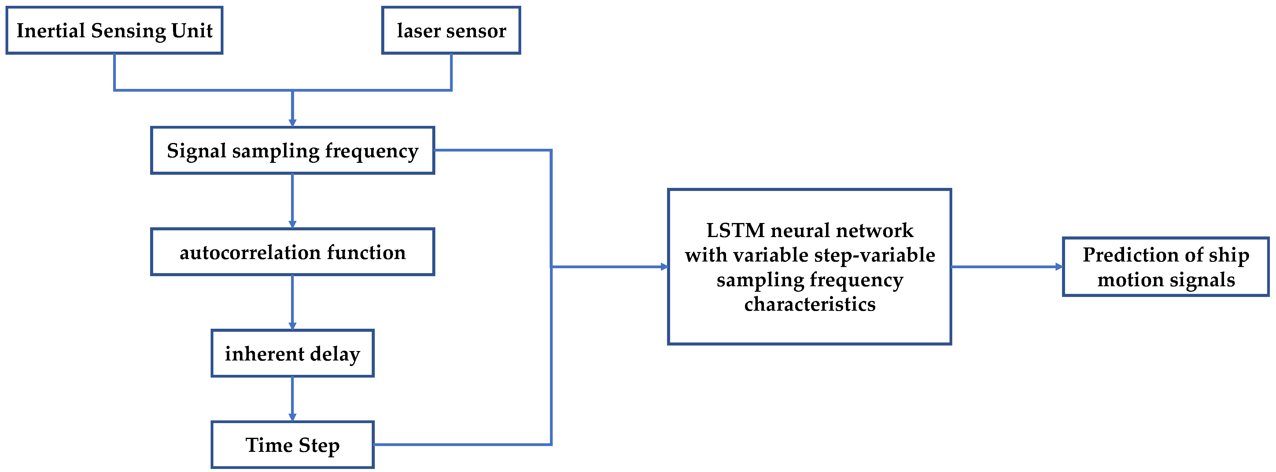
The flow chart of the ship motion signal prediction method is shown in Figure 4, and the schematic diagram of the LSTM neural network with variable step-variable sampling frequency characteristics is shown in Figure 5.

4. Experimental Results and Analysis

We designed an experiment to verify the prediction accuracy of the LSTM neural network with variable step-variable sampling frequency characteristics for ship motion signals. The experiment is divided into two parts: 1. use the cross-correlation analysis of the reference signal and the displacement signal to calculate the inherent delay of the ship motion measurement system; 2. use the LSTM neural network with variable step-variable sampling frequency characteristics to predict the ship motion signal within the inherent delay of the measurement system.

4.1. Calculation of Inherent Delay in Ship Motion Measurement System

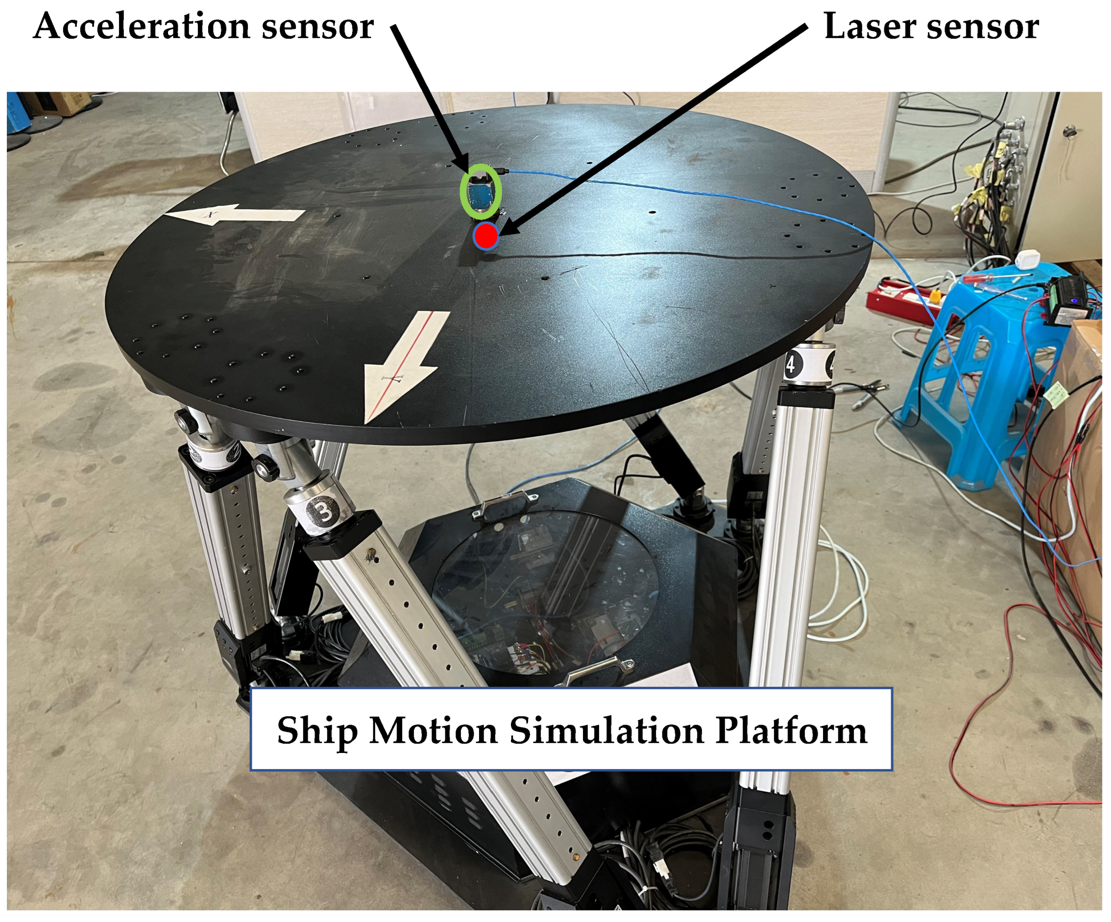
The existing ship motion measurement system currently used in the laboratory is mainly composed of an acceleration sensor and a secondary integration box. The acceleration sensor is responsible for inputting acceleration signals for the system, and the secondary integration box is for the system to output ship displacement. The acceleration sensor in the ship motion measurement system is installed on a six-degree-of-freedom platform to collect heave motion signals. At the same time, the laser sensor is used to collect the reference heave signal, which is also installed on the six-degree-of-freedom platform. In the following text, the acceleration sensor and the ship motion measurement system represents the same concept. The placement of the two sensors is shown in Figure 6.
Using the six-free platform to imitate the irregular vertical heave motion of the ship, we collected and analyzed the displacement signal of the laser sensor and the integral signal of the acceleration sensor. We observed whether there was a time delay in the integral signal of the acceleration sensor and the displacement signal of the laser sensor. We set the signal sampling frequency of the signal collector to 100 Hz, the collection time to 200 s, and we collected 4 groups of motion signals. The real-time waveforms output by the acceleration sensor and the laser sensor were displayed in the host computer, as shown in Figure 7.
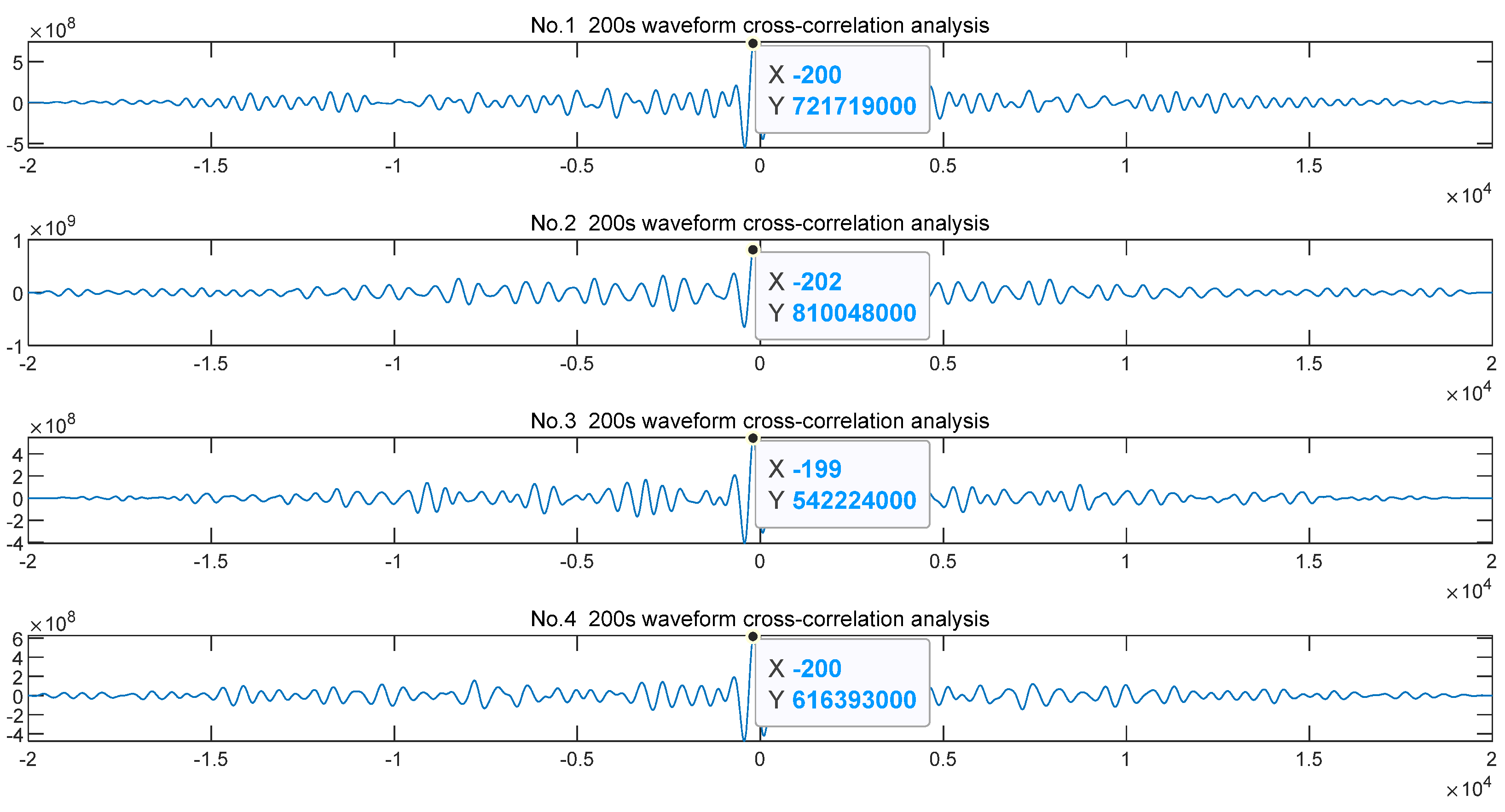
After analysis, it was found that when the laser sensor collects the motion signal of the six-degree-of-freedom platform, it could respond to the heave motion of the platform in real time, which meets the conditions of the reference signal. The acceleration signal collected by the acceleration sensor is integrated into the displacement signal, and the laser signal had an obvious phase lag, which verified that the integral calculation time in the acquisition module of the active wave compensation system will cause the lag of the acquisition signal. The acceleration sensor displacement signal and the laser sensor displacement signal were processed for cross-correlation analysis, and the results are shown in Figure 8.
It can also be seen from the cross-correlation analysis that there was a hysteresis relationship between the displacement signal integrated by the acceleration sensor and the displacement signal collected by the laser sensor. According to the results of the cross-correlation analysis, the displacement sequence collected by the acceleration sensor and the displacement sequence collected by the laser sensor have a dislocation in the range of [−199, −202]. At the average dislocation point of 200, the matching degree of the two displacement signal sequences was the highest. Since the sampling frequency of the signal collector was 100 Hz, it was calculated that the average inherent delay of the ship motion measurement system was about 2 s. Therefore, it is only necessary to predict the heave signal of the ship within the inherent delay of 2 s, and the accurate collection of the heave displacement of the ship can be realized.

4.2. Calculation of Inherent Delay in Ship Motion Measurement System

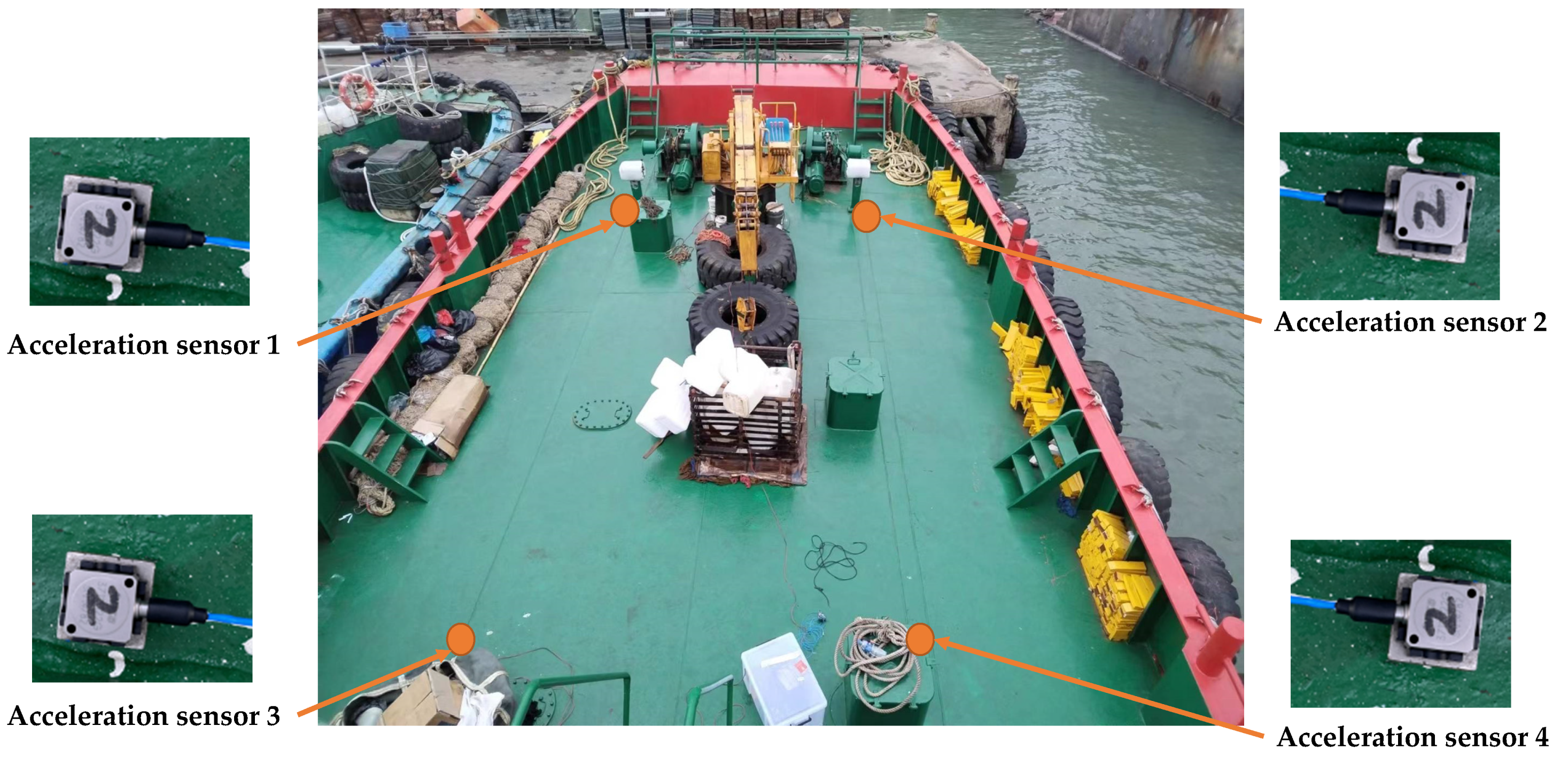
We set up a ship motion measurement system on a catamaran in a dock in Guangdong Province. The system mainly included four acceleration sensors, a secondary integration box, a signal collector, and other hardware equipment. The system had a total of 12 acquisition channels, setting a variety of different sampling frequencies, and the sampling time is 1000 s. The acceleration sensor was installed on the deck plane of the ship, and the specific collection position is shown in Figure 9.
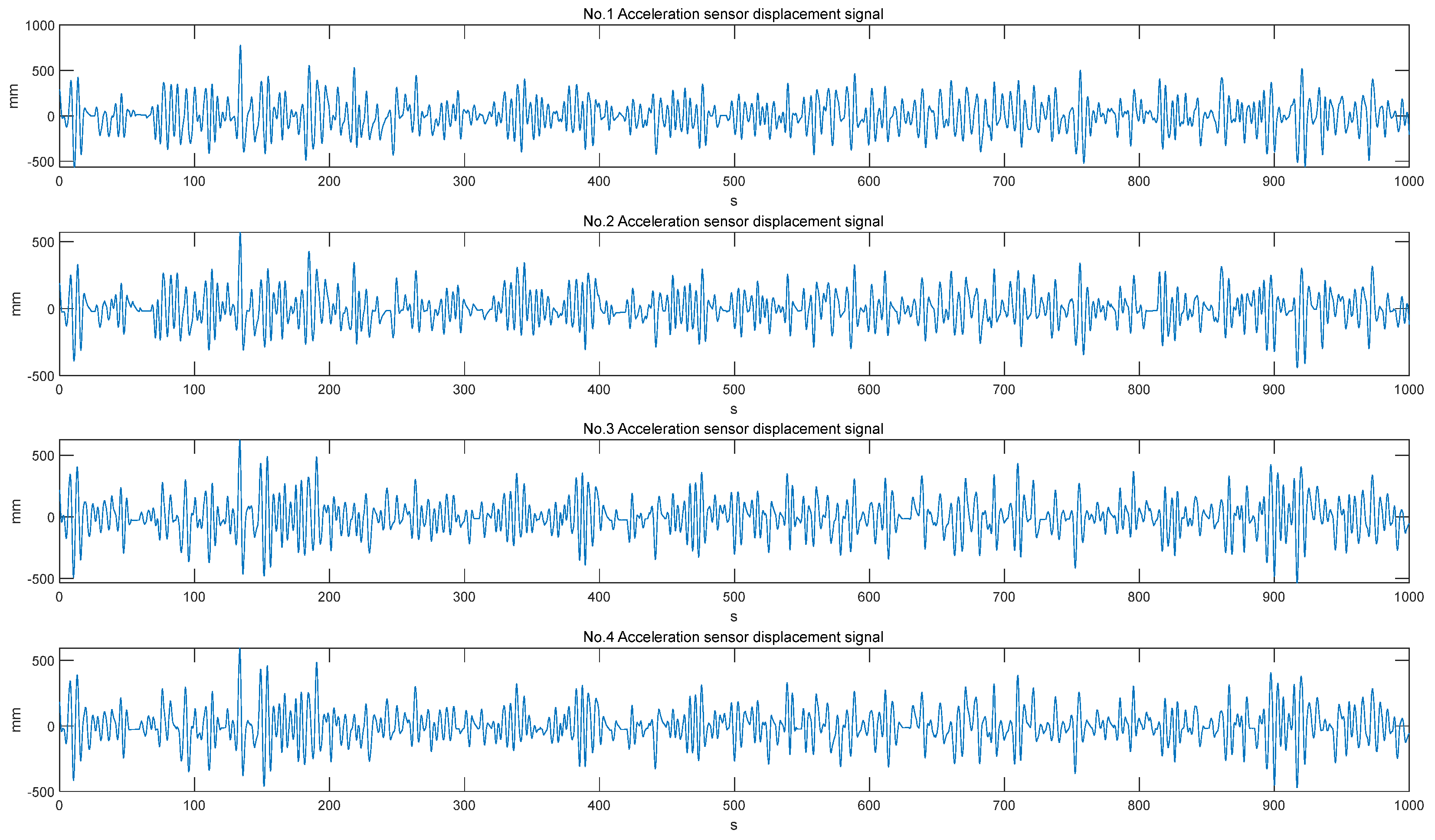
The acceleration signal collected by the acceleration sensor was used as the input of the secondary integrator. Each integrator outputs a filtered acceleration signal, an integrated velocity signal, and a second-integrated displacement signal. Each sensor occupied 3 channels, for a total of 12 channels. The analog signals of 12 channels were converted into digital signals by the signal collector and displayed on the host computer. Finally, the ship heave displacement signals of the 4 channels are obtained, as shown in Figure 10.
In the actual measurement process, the integration of the acceleration sensor will produce a trend term. At the same time, the low-frequency characteristics of ship motion will cause serious low-frequency baseline drift of the integral displacement signal (the so-called baseline drift refers to the non-zero offset, oscillation and other distortions of the center line axis obtained from the acceleration integration to obtain the velocity and displacement). The generated trend items will accumulate over time, causing the error to gradually increase. Therefore, a reset step is generally added to the acceleration sensor integration step to eliminate the influence of the trend items. This trend item leads to a long-term characteristic of the signal collected by the acceleration sensor. Therefore, in the training data of the LSTM neural network, it is necessary to include the long-term integration of the acceleration sensor characteristics, but to also include the short-term period characteristics of ship motion.
According to the long-term and short-term characteristics of ship motion, a training set and a test set are constructed based on the signals collected by the above-mentioned ship motion measurement system.
Build the training set according to the sampling frequency: The length of the input data of the training set was [1 s–400 s] data collected by the acceleration sensor. The length of the output data of the training set was [1 s–400 s] lagging data, which lags behind the inherent delay time. The input data dimension of the training set was a 4-dimensional array, that is, the data of 4 sets of acceleration sensors. The output data dimension of the training set was a 1-dimensional array, which is the average value of the 4 sets of acceleration sensor data. In each set of experiments, different sampling frequencies lead to different data vectors along the length of the data set. Using a data volume of 400 s not only ensures that the long-term integral characteristic knowledge of the acceleration sensor can be memorized by the network, but also ensures the short-term period characteristic of the ship motion.
Build the testing set based on the same parameters as the training set: The length of the input data of the testing set was [101 s–500 s] data collected by the acceleration sensor. The length of the output data of the testing set was [101 s–500 s] lagging data, which lags behind the inherent delay time. The size of the testing set data dimension was the same as the training set data dimension size. In the output results predicted by the LSTM model, different sampling frequencies correspond to different prediction steps. By constructing the test set with an interval of 100 s, the ship motion information of [101 s–400 s] can be retained, which allows the cell state of LSTM to be updated better. At the same time, [401 s–500 s] was new ship motion data, which makes the predicted results more reliable.
In Section 4.1, we have calculated that the inherent delay of the ship motion measurement system used in this experiment is 2 s. According to the inherent delay, eight groups of LSTM neural networks with variable step-variable sampling frequency characteristics were constructed to compensate the signal lost by the ship motion acquisition system within 2 s. The characteristic parameters of the network are shown in Table 1.
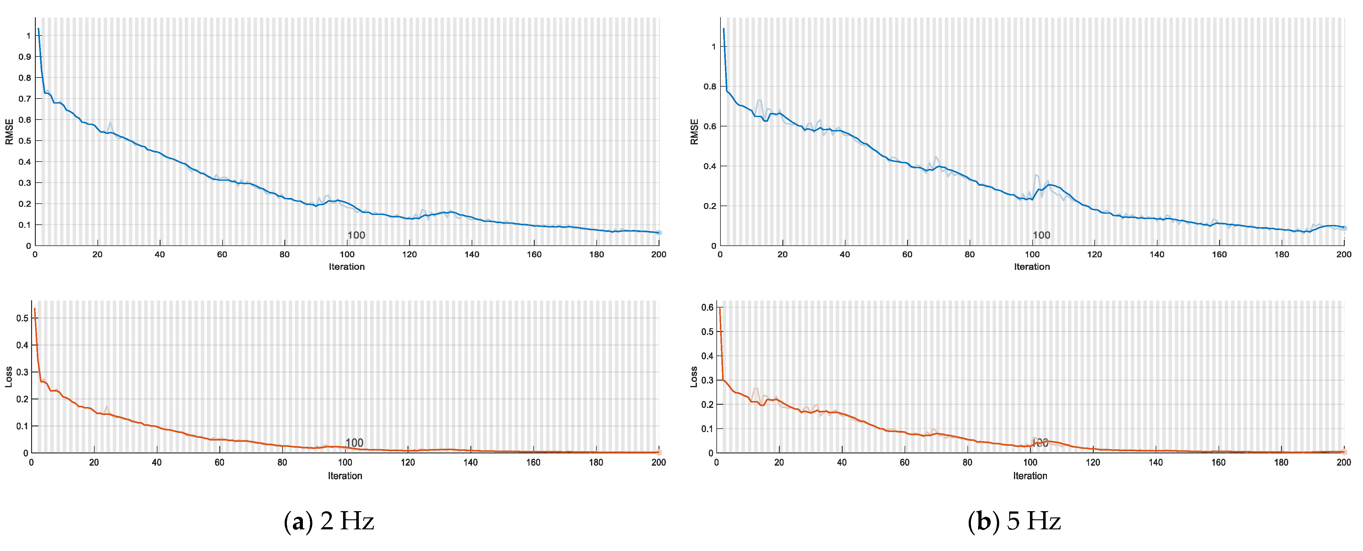
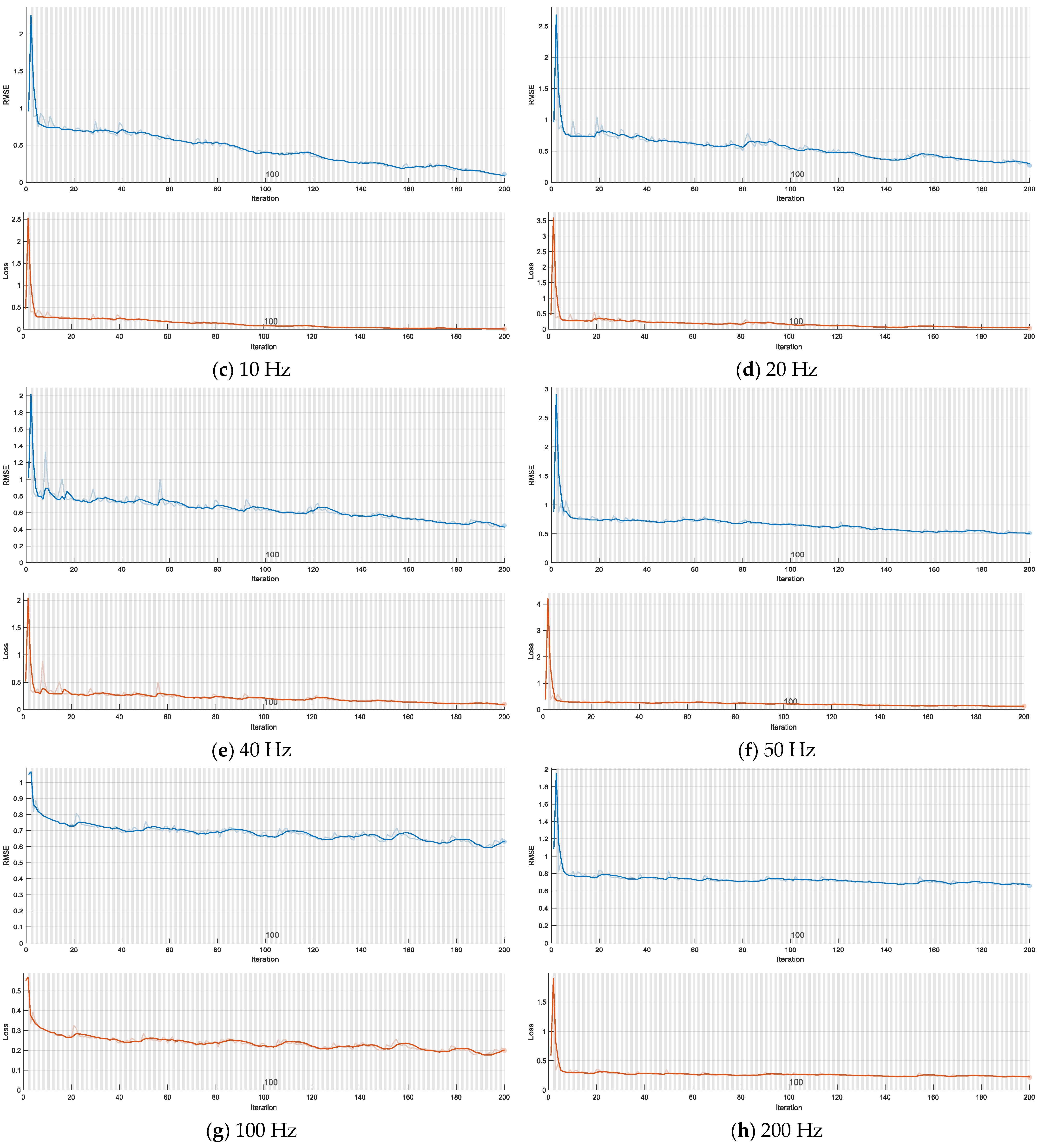
Corresponding to the different sampling frequencies in Table 1, the LSTM neural network was trained separately. The number of neuron nodes in the input layer of the network was 4, the number of neuron nodes in the hidden layer was 100, and the number of neuron nodes in the output layer was 4. The network training results are shown in Figure 11.
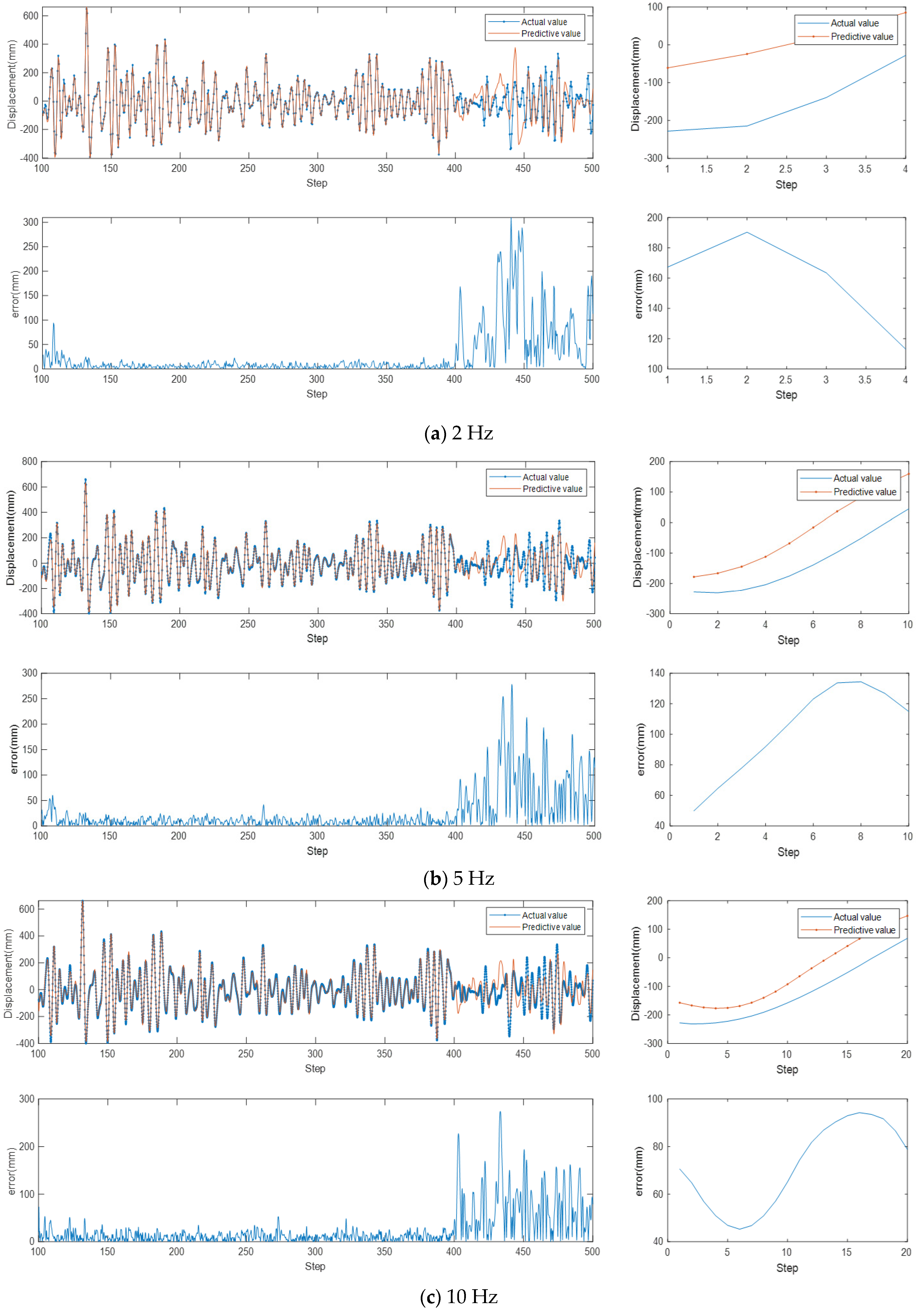
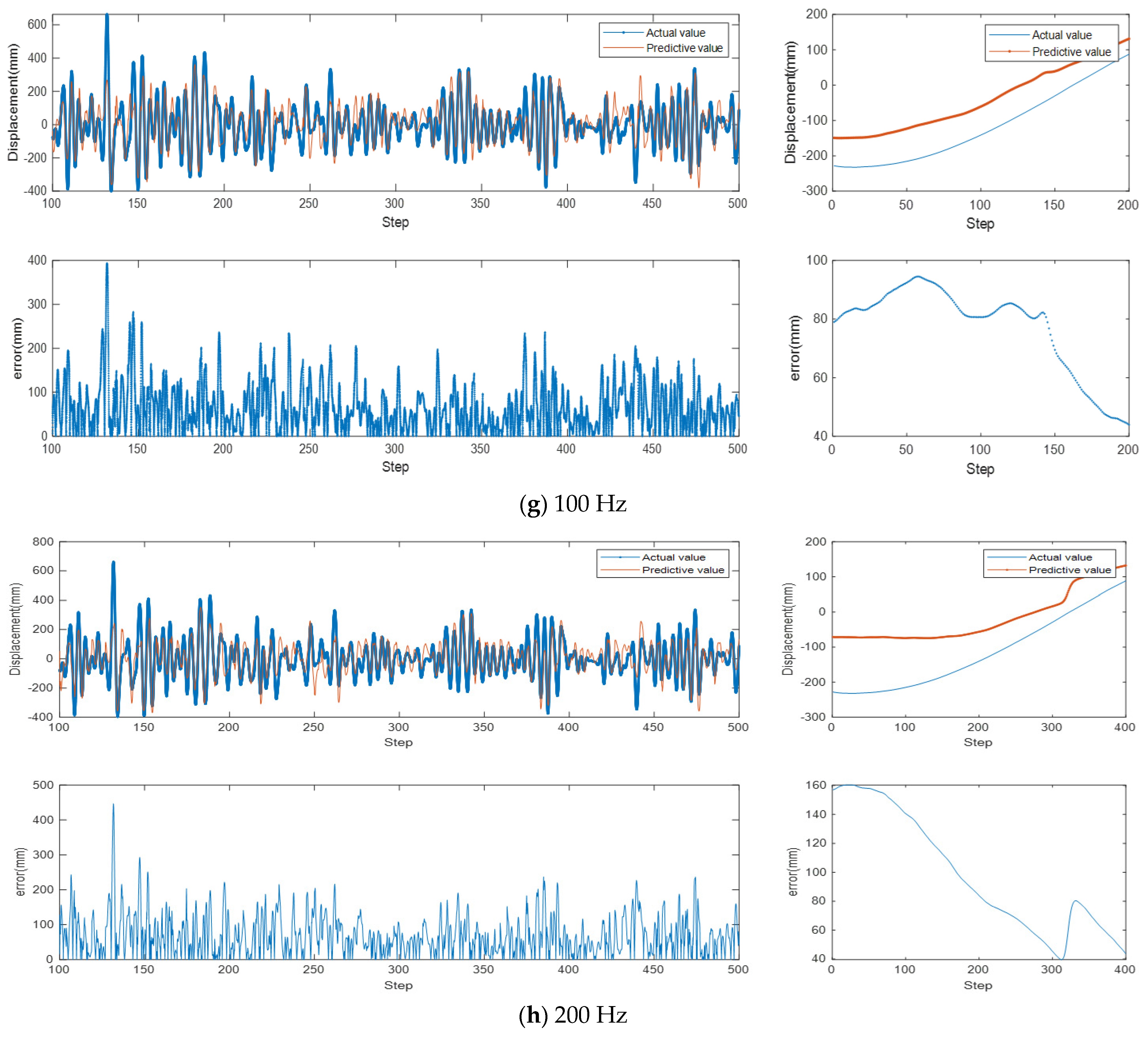
After the training of the LSTM neural network with variable step-variable sampling frequency characteristics is completed, the prediction effect is checked on the test set. The results of the eight groups of predictions and the errors of the predictions are shown in Figure 12.
The experimental results show that the prediction accuracy of 8 groups of sampling frequencies [2 Hz, 5 Hz, 10 Hz, 20 Hz, 40 Hz, 50 Hz, 100 Hz, 200 Hz] corresponding to 8 groups of inherent delay time steps [4, 10, 20, 40, 80, 100, 200, 400] is:
  • Hz = 2, Step = 4, the average prediction error of the ship motion signal within 2 s of the inherent delay is 158.53 mm, and the average prediction error of the overall duration is 27.16 mm. The prediction accuracy of the model for the signal within the inherent delay is 72.66%;
  • Hz = 5, Step = 10, the average prediction error of the ship motion signal within 2 s of the inherent delay is 102.41 mm, and the average prediction error of the overall duration is 25.58 mm. The prediction accuracy of the model for the signal within the inherent delay is 82.34%;
  • Hz = 10, Step = 20, the average prediction error of the ship motion signal within 2 s of the inherent delay is 71.31 mm, and the average prediction error of the overall duration is 26.21 mm. The prediction accuracy of the model for the signal within the inherent delay is 87.71%;
  • Hz = 20, Step = 40, the average prediction error of the ship motion signal within 2 s of the inherent delay is 18.85 mm, and the average prediction error of the overall duration is 38.29 mm. The prediction accuracy of the model for the signal within the inherent delay is 96.75%;
  • Hz = 40, Step = 80, the average prediction error of the ship motion signal within 2 s of the inherent delay is 22.38 mm, and the average prediction error of the overall duration is 51.78 mm. The prediction accuracy of the model for the signal within the inherent delay is 96.14%;
  • Hz = 50, Step = 100, the average prediction error of the ship motion signal within 2 s of the inherent delay is 39.83 mm, and the average prediction error of the overall duration is 58.52 mm. The prediction accuracy of the model for the signal within the inherent delay is 93.13%;
  • Hz = 100, Step = 200, the average prediction error of the ship motion signal within 2 s of the inherent delay is 77.11 mm, and the average prediction error of the overall duration is 66.63 mm. The prediction accuracy of the model for the signal within the inherent delay is 86.71%;
  • Hz = 200, Step = 400, the average prediction error of the ship motion signal within 2 s of the inherent delay is 98.32 mm, and the average prediction error of the overall duration is 69.98 mm. The prediction accuracy of the model for the signal within the inherent delay is 83.04%;
Summarizing the above results, it can be obtained that the accuracy of predicting ship motion signals using the LSTM neural network with variable step-variable sampling frequency characteristics is [72.66–96.75%], which verifies that the prediction accuracy is related to the sampling frequency and the prediction step of the LSTM neural network.

4.3. Experimental Discussion

Through these experiments, it can be concluded that the motion of the ship was simulated by the heave platform in the laboratory, and the displacement signal of the motion platform was measured simultaneously by the ship motion measurement system and the laser sensor system, which verifies that the ship motion measurement system does have an inherent delay. Secondly, on the marine ship, the ship displacement signal was collected by setting up four sets of ship motion measurement systems. Finally, different parameters were set, and the LSTM neural network with variable step-variable sampling frequency characteristics was used to predict the motion of the ship, which verifies that the prediction accuracy is related to the sampling frequency of the signal collector and the prediction step of the LSTM neural network.
When the sampling frequency of the ship motion signal was low, the training speed of the LSTM neural network model was fast, the convergence effect was better, and the model could learn well the short-term characteristics of the ship motion cycle in the training samples. However, due to the low sampling frequency, the number of training samples was relatively small, the time steps for the prediction of the inherent delay were small, and the learning of the long-term characteristics of the acceleration sensor was poor, which ultimately made the prediction error for the inherent delay larger.
When the sampling frequency of the ship motion signal was high, the model could learn well the long-term characteristics of the acceleration sensor in the training samples. However, due to the high sampling frequency, the number of training samples was so large that the training speed of the LSTM neural network model was slow and the convergence effect was poor. In addition, there were many time steps in the prediction of the inherent delay, and the learning of the short-term characteristics of the ship’s motion cycle was poor, which ultimately made the prediction error of the inherent delay larger. Therefore, choosing an appropriate sampling frequency and time step can balance the learning effect of long and short time characteristics in the ship motion signal, and improve the prediction accuracy of the model and the timeliness of ship motion acquisition.
Predicting ship movements through an LSTM neural network with variable step-variable sampling frequency characteristics can help crews better plan routes, avoid potentially dangerous situations, and reduce fuel consumption. In addition, the model can also monitor the power usage of the ship in real time, thereby optimizing the energy utilization efficiency of the ship and reducing operating costs. In conclusion, using an LSTM neural network with variable step-variable sampling frequency characteristics to predict ship motion has broad application prospects and can bring many advantages to ship operations.

5. Conclusions

This paper proposed a ship motion signal prediction method based on an LSTM neural network with variable step-variable sampling frequency characteristics. At the same time, the autocorrelation function was used to conduct cross-correlation analysis on the ship motion collected by the ship motion measurement system and the laser sensor, and the inherent delay of the ship motion measurement system could be accurately obtained. Based on multiple sets of sampling frequencies and multiple sets of prediction steps, the LSTM neural network was built to predict the ship motion signal within the inherent delay time and realize the prediction of the ship motion signal within the inherent delay time.
The advantage of this method was that the inherent time delay of the ship motion measurement system could be accurately calculated according to the cross-correlation analysis, and the ship motion signal could be measured more accurately. During the transportation of the wind power generation equipment, the hidden danger caused by the delay problem of the measurement system was eliminated, and the real-time performance of the measurement of the ship motion signal could be improved. The results showed that the sampling frequency and prediction step have an impact on the prediction accuracy, and balancing the long-term integral characteristics of acceleration and the short-term period characteristics of ship motion can improve the prediction accuracy.
The disadvantage of this method was that it only solved the inherent delay for the ship motion measurement system in the laboratory and does not accurately balance the long and short time characteristics in the ship motion signal data.
In the current work, the ship motion measurement system we built was only for the heave displacement of the ship. In future work, we will further study the delay problem in the process of ship displacement signal measurement, seeking the system lag from the whole active heave compensation system. At the same time, in order to solve the measurement lag and control lag of the system, we will focus on lag control, fuzzy control, and other technologies.

Author Contributions

Conceptualization, C.H. and X.H.; methodology, C.H.; software, C.H.; writing—original draft preparation, C.H.; writing—review and editing, X.H.; supervision, X.H. All authors have read and agreed to the published version of the manuscript.

Funding

This research was funded by the National Natural Science Foundation of China grant number 31300783.

Institutional Review Board Statement

Not applicable.

Informed Consent Statement

Not applicable.

Data Availability Statement

The original data contributions presented in the study are included in the article; further inquiries can be directed to the corresponding authors.

Conflicts of Interest

The authors declare no conflict of interest.

References

  1. Woodacre, J.K.; Bauer, R.J.; Irani, R.A. A Review of Vertical Motion Heave Compensation Systems. Ocean Eng. 2015, 104, 140–154. [Google Scholar] [CrossRef]
  2. Hatleskog, J.T.; Dunnigan, M.W. Heave Compensation Simulation for Non-Contact Operations in Deep Water. In Proceedings of the OCEANS 2006, Boston, MA, USA, 18–21 September 2006; pp. 1–6. [Google Scholar]
  3. Do, K.D.; Pan, J. Nonlinear Control of an Active Heave Compensation System. Ocean Eng. 2008, 35, 558–571. [Google Scholar] [CrossRef]
  4. Küchler, S.; Sawodny, O. Nonlinear Control of an Active Heave Compensation System with Time-Delay. In Proceedings of the 2010 IEEE International Conference on Control Applications, Yokohama, Japan, 8–10 September 2010; pp. 1313–1318. [Google Scholar]
  5. Kyllingstad, A. Method and Apparatus for Active Heave Compensation. U.S. Patent 8,265,811, 11 September 2012. [Google Scholar]
  6. Küchler, S.; Mahl, T.; Neupert, J.; Schneider, K.; Sawodny, O. Active Control for an Offshore Crane Using Prediction of the Vessel’s Motion. IEEE/ASME Trans. Mechatron. 2010, 16, 297–309. [Google Scholar] [CrossRef]
  7. Liu, J.; Chen, X. Adaptive Control Based on Neural Network and Beetle Antennae Search Algorithm for an Active Heave Compensation System. Int. J. Control Autom. Syst. 2022, 20, 515–525. [Google Scholar] [CrossRef]
  8. Richter, M.; Arnold, E.; Schneider, K.; Eberharter, J.K.; Sawodny, O. Model Predictive Trajectory Planning with Fallback-Strategy for an Active Heave Compensation System. In Proceedings of the 2014 American Control Conference, Portland, OR, USA, 4–6 June 2014; pp. 1919–1924. [Google Scholar]
  9. Chu, Y.; Li, G.; Zhang, H. Incorporation of Ship Motion Prediction into Active Heave Compensation for Offshore Crane Operation. In Proceedings of the 2020 15th IEEE Conference on Industrial Electronics and Applications (ICIEA), Kristiansand, Norway, 9–13 November 2020; pp. 1444–1449. [Google Scholar]
  10. Hu, L.; Zhang, M.; Yuan, Z.M.; Zheng, H.; Lv, W. Predictive control of a heaving compensation system based on machine learning prediction algorithm. J. Mar. Sci. Eng. 2023, 11, 821. [Google Scholar] [CrossRef]
  11. Richter, M.; Schaut, S.; Walser, D.; Schneider, K.; Sawodny, O. Experimental Validation of an Active Heave Compensation System: Estimation, Prediction and Control. Control Eng. Pract. 2017, 66, 1–12. [Google Scholar] [CrossRef]
  12. Neupert, J.; Mahl, T.; Haessig, B.; Sawodny, O.; Schneider, K. A Heave Compensation Approach for Offshore Cranes. In Proceedings of the 2008 American Control Conference, Seattle, WA, USA, 11–13 June 2008; pp. 538–543. [Google Scholar]
  13. Woodacre, J.K.; Bauer, R.J.; Irani, R. Hydraulic Valve-Based Active-Heave Compensation Using a Model-Predictive Controller with Non-Linear Valve Compensations. Ocean Eng. 2018, 152, 47–56. [Google Scholar] [CrossRef]
  14. Shi, B.; Xian, L.; Wu, Q.; Zhang, Y. Active Heave Compensation Prediction Research for Deep Sea Homework Crane Based on KPSO-SVR. In Proceedings of the 33rd Chinese Control Conference, Nanjing, China, 28–30 July 2014; pp. 7637–7642. [Google Scholar]
  15. Li, G.; Kawan, B.; Wang, H.; Zhang, H. Neural-Network-Based Modelling and Analysis for Time Series Prediction of Ship Motion. Ship Technol. Res. 2017, 64, 30–39. [Google Scholar] [CrossRef]
  16. De Masi, G.; Gaggiotti, F.; Bruschi, R.; Venturi, M. Ship Motion Prediction by Radial Basis Neural Networks. In Proceedings of the 2011 IEEE Workshop on Hybrid Intelligent Models and Applications, Paris, France, 11–15 April 2011; pp. 28–32. [Google Scholar]
  17. Skulstad, R.; Li, G.; Fossen, T.I.; Vik, B.; Zhang, H. A Hybrid Approach to Motion Prediction for Ship Docking—Integration of a Neural Network Model into the Ship Dynamic Model. IEEE Trans. Instrum. Meas. 2020, 70, 1–11. [Google Scholar] [CrossRef]
  18. Khan, A.; Bil, C.; Marion, K.E. Theory and Application of Artificial Neural Networks for the Real Time Prediction of Ship Motion. In Proceedings of the Knowledge-Based Intelligent Information and Engineering Systems: 9th International Conference, KES 2005, Melbourne, Australia, 14–16 September 2005; Proceedings, Part I 9. Springer: Berlin/Heidelberg, Germany, 2005; pp. 1064–1069. [Google Scholar]
  19. Yao, Y.; Han, L.; Wang, J. Lstm-Pso: Long Short-Term Memory Ship Motion Prediction Based on Particle Swarm Optimization. In Proceedings of the 2018 IEEE CSAA Guidance, Navigation and Control Conference (CGNCC), Xiamen, China, 10–12 August 2018; pp. 1–5. [Google Scholar]
  20. Zhang, G.; Tan, F.; Wu, Y. Ship Motion Attitude Prediction Based on an Adaptive Dynamic Particle Swarm Optimization Algorithm and Bidirectional LSTM Neural Network. IEEE Access 2020, 8, 90087–90098. [Google Scholar] [CrossRef]
  21. Liu, Y.; Duan, W.; Huang, L.; Duan, S.; Ma, X. The Input Vector Space Optimization for LSTM Deep Learning Model in Real-Time Prediction of Ship Motions. Ocean Eng. 2020, 213, 107681. [Google Scholar] [CrossRef]
  22. Duan, S.; Ma, Q.; Huang, L.; Ma, X. A LSTM Deep Learning Model for Deterministic Ship Motions Estimation Using Wave-Excitation Inputs. In Proceedings of the 29th International Ocean and Polar Engineering Conference, Honolulu, HI, USA, 16–21 June 2019. [Google Scholar]
  23. Sun, Q.; Tang, Z.; Gao, J.; Zhang, G. Short-Term Ship Motion Attitude Prediction Based on LSTM and GPR. Appl. Ocean Res. 2022, 118, 102927. [Google Scholar] [CrossRef]
  24. Zhang, T.; Zheng, X.-Q.; Liu, M.-X. Multiscale Attention-Based LSTM for Ship Motion Prediction. Ocean Eng. 2021, 230, 109066. [Google Scholar] [CrossRef]
  25. Su, Y.; Lin, J.; Zhao, D.; Guo, C.; Wang, C.; Guo, H. Real-Time Prediction of Large-Scale Ship Model Vertical Acceleration Based on Recurrent Neural Network. J. Mar. Sci. Eng. 2020, 8, 777. [Google Scholar] [CrossRef]
  26. Wang, Y.; Wang, H.; Zou, D.; Fu, H. Ship Roll Prediction Algorithm Based on Bi-LSTM-TPA Combined Model. J. Mar. Sci. Eng. 2021, 9, 387. [Google Scholar] [CrossRef]
  27. Huang, L.; Deng, X.; Bo, Y.; Zhang, Y.; Wang, P. Evolutionary Optimization Assisted Delayed Deep Cycle Reservoir Modeling Method with Its Application to Ship Heave Motion Prediction. ISA Trans. 2022, 126, 638–648. [Google Scholar] [CrossRef] [PubMed]
  28. Guo, W.; Piao, S.; Guo, J.; Lei, Y.; Iqbal, K. Passive Detection of Ship-Radiated Acoustic Signal Using Coherent Integration of Cross-Power Spectrum with Doppler and Time Delay Compensations. Sensors 2020, 20, 1767. [Google Scholar] [CrossRef] [PubMed]
  29. Gao, F.; Xu, T.; Wang, N.; He, Y.; Luo, X. A Shipborne Experiment Using a Dual-Antenna Reflectometry System for GPS/BDS Code Delay Measurements. J. Geod 2020, 94, 88. [Google Scholar] [CrossRef]
  30. Hu, T.; Xu, Q.; Huang, G.; Nie, Y. Adaptive Time Delay Compensation Realization for Remote Ship Main Engine Rotation Measurement. In Proceedings of the 2016 International Conference on Education, Management and Computer Science, Shenyang, China, 27–29 May 2016; Atlantis Press: Amsterdam, The Netherlands, 2016; pp. 34–38. [Google Scholar]
  31. Abebe, M.; Noh, Y.; Kang, Y.-J.; Seo, C.; Kim, D.; Seo, J. Ship Trajectory Planning for Collision Avoidance Using Hybrid ARIMA-LSTM Models. Ocean Eng. 2022, 256, 111527. [Google Scholar] [CrossRef]
  32. Zhang, Z.; Ni, G.; Xu, Y. Ship Trajectory Prediction Based on LSTM Neural Network. In Proceedings of the 2020 IEEE 5th Information Technology and Mechatronics Engineering Conference (ITOEC), Chongqing, China, 12–14 June 2020; pp. 1356–1364. [Google Scholar]
  33. Kaklis, D.; Eirinakis, P.; Giannakopoulos, G.; Spyropoulos, C.; Varelas, T.J.; Varlamis, I. A Big Data Approach for Fuel Oil Consumption Estimation in the Maritime Industry. In Proceedings of the 2022 IEEE Eighth International Conference on Big Data Computing Service and Applications (BigDataService), Newark, CA, USA, 15–18 August 2022; pp. 39–47. [Google Scholar]
  34. Kaklis, D.; Varelas, T.J.; Varlamis, I.; Eirinakis, P.; Giannakopoulos, G.; Spyropoulos, C. V From STEAM to Machine: Emissions Control in the Shipping 4.0 Era. In Proceedings of the SNAME 8th International Symposium on Ship Operations, Management and Economics, Athens, Greece, 7–8 March 2023. [Google Scholar]
  35. Kaklis, D.; Varlamis, I.; Giannakopoulos, G.; Spyropoulos, C.; Varelas, T.J. Online Training for Fuel Oil Consumption Estimation: A Data Driven Approach. In Proceedings of the 2022 23rd IEEE International Conference on Mobile Data Management (MDM), Paphos, Cyprus, 6–9 June 2022; pp. 394–400. [Google Scholar]
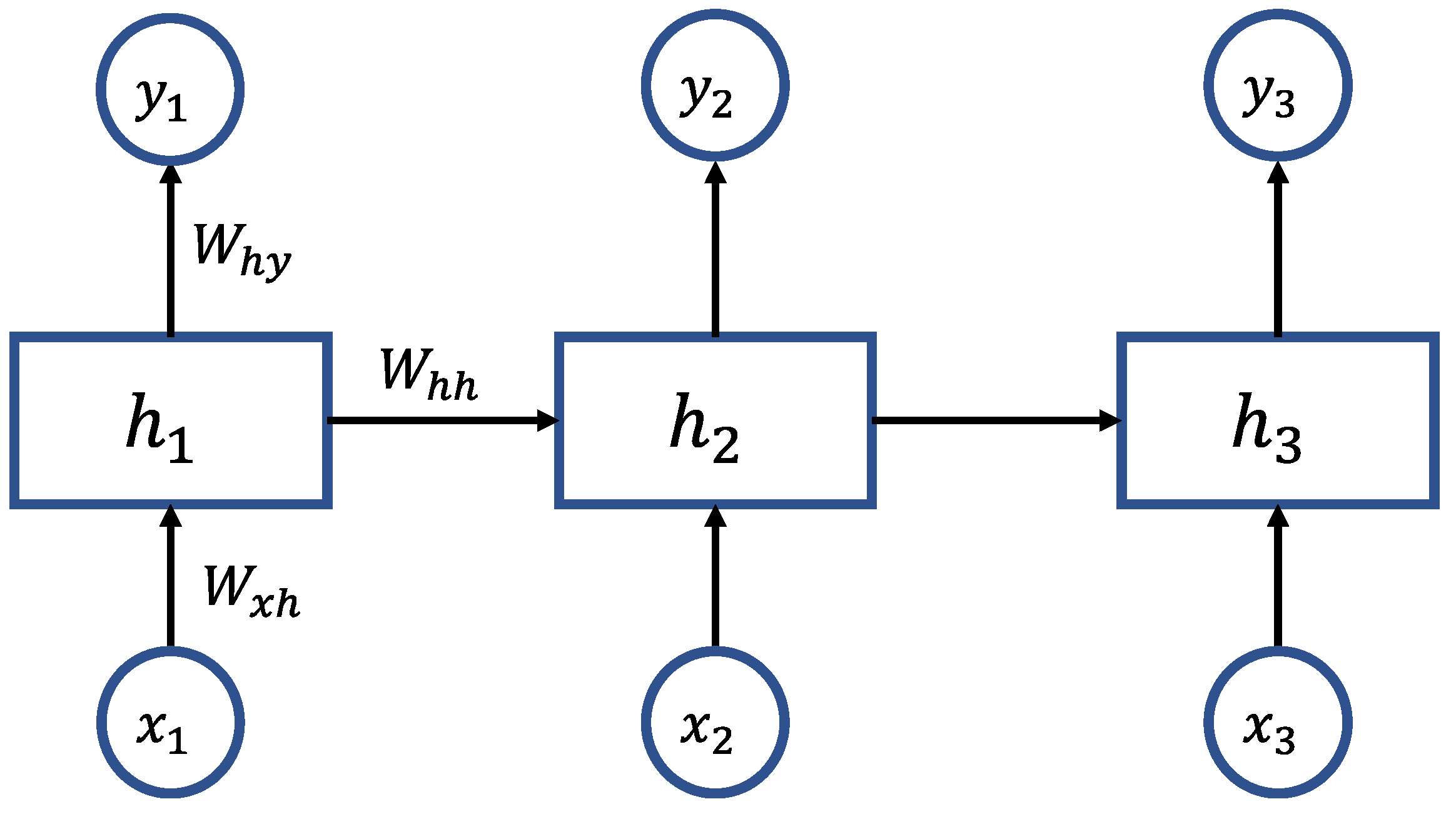
Figure 1. Structural form diagram of the Recurrent Neural Network.
Jmse 11 00919 g001
Figure 2. Structural form diagram of the LSTM Neural Network.
Jmse 11 00919 g002
Figure 3. Structural flowchart of the solution for inherent delay in the ship motion measurement system.
Jmse 11 00919 g003
Figure 4. The flow chart of the ship motion signal prediction method.
Jmse 11 00919 g004
Figure 5. The schematic diagram of the LSTM neural network with variable step-variable sampling frequency characteristics.
Jmse 11 00919 g005
Figure 6. Schematic diagram of the installation of the sensor on the heave platform.
Jmse 11 00919 g006
Figure 7. Waveform diagram of four sets of displacement signals collected by two sensors.
Jmse 11 00919 g007
Figure 8. Cross-correlation analysis results of the laser displacement signal and integral displacement signal.
Jmse 11 00919 g008
Figure 9. Measuring point layout diagram of four ship motion measuring systems.
Jmse 11 00919 g009
Figure 10. Waveform diagram of 1000 s ship heave displacement signals collected by 4 ship motion measurement systems.
Jmse 11 00919 g010
Figure 11. LSTM neural network training process diagram with different sampling frequencies, results of loss function and RMSE.
Jmse 11 00919 g011aJmse 11 00919 g011b
Figure 12. The prediction results of eight groups of LSTM neural networks with variable step-variable sampling frequency characteristics within the inherent delay, and the result of the prediction error.
Jmse 11 00919 g012aJmse 11 00919 g012bJmse 11 00919 g012c
Table 1. The characteristic parameters of the LSTM neural network.
No.Sampling FrequencyLong-Term CharacteristicsShort-Term CharacteristicsPrediction Step
12 Hz400 s × 2 Hz2 s × 2 Hz4
25 Hz400 s × 5 Hz2 s × 5 Hz10
310 Hz400 s × 10 Hz2 s × 10 Hz20
420 Hz400 s × 20 Hz2 s × 20 Hz40
540 Hz400 s × 40 Hz2 s × 40 Hz80
650 Hz400 s × 50 Hz2 s × 50 Hz100
7100 Hz400 s × 100 Hz2 s × 100 Hz200
8200 Hz400 s × 200 Hz2 s × 200 Hz400
Disclaimer/Publisher’s Note: The statements, opinions and data contained in all publications are solely those of the individual author(s) and contributor(s) and not of MDPI and/or the editor(s). MDPI and/or the editor(s) disclaim responsibility for any injury to people or property resulting from any ideas, methods, instructions or products referred to in the content.