A Multidecadal Assessment of Mean and Extreme Wave Climate Observed at Buoys off the U.S. East, Gulf, and West Coasts

Abstract

The current understanding of wind-generated wave climate from buoy-based measurements is mainly focused on a limited number of locations and has not been updated to include measurements in the past decade. This study quantifies wave climate variability and change during the historical period of 1980–2020 through a comprehensive analysis of wave height measurements at 43 buoys off the U.S. Pacific, Atlantic, and Gulf of Mexico Coasts. Variabilities and trends in the annual and monthly mean and 95th percentile significant wave heights (SWH) and the number of extreme wave events are quantified for the cold and warm seasons. We calculate the SWH long-term and decadal trends, and temporal variabilities using the ordinary least squares regression and coefficient of variation, respectively. Independent extreme wave events are identified using a method based on the peaks-over-threshold and the autocorrelation function, which accounts for the geographical variation in the timespan between independent extreme events. Results show that the warm season’s interannual variabilities in monthly and annual SWH are smaller in the Pacific while larger in the Atlantic and Gulf, with the largest variabilities observed at buoys in the Gulf and lower latitudes of the Atlantic. Strong significant alternating decadal trends in SWH are found in the Pacific and Atlantic regions. Buoys in the Atlantic and Gulf regions have experienced higher numbers of extreme wave events (anomalies) compared to the Pacific region. In general, the long-term trend in the number of extreme events during the cold season is positive at buoys located at higher latitudes but negative at lower latitudes.

1. Introduction

Due to their direct impact on the coastal regions and offshore structures, extreme wind-generated ocean waves have gained increasing attention in the research community in the past century. The effect of extreme waves manifests itself in different forms of impact including erosion and inundation of beach–dune systems [1], overtopping of coastal and offshore structures such as seawalls [2], harbors [3,4], and gas and oil production systems [5]. Hurricane-induced extreme waves are among the other major threats that affect coastal regions as they can cause extensive erosion and flooding of coastal urban regions. For example, the eroded volumes from Hurricane Sandy along the New Jersey coastline ranged between 30–160 m³/m above the mean sea level [6]. An important aspect of waves is their spatiotemporal variability and changing trends. A quantitative understanding of trends and spatial and temporal variabilities in the wave climate is beneficial to better understand and predict natural oceanic processes and social and economic impacts from wind waves. To that end, researchers have been analyzing wave time series data from different sources.

In situ buoy, altimeter, numerical model hindcast, and reanalysis data have been analyzed to understand the wave climate and its variability and change. For example, refs. [7,8] analyzed altimeter radar to quantify global wave statistics of mean monthly significant wave height (SWH) and wind speed for a temporal scale of 3 years. Ref. [9] examined the direction and magnitude of SWH and wind and mean and peak wave periods using a longer record of altimeter data (10 years). Ref. [10] further investigated global trends in extreme wave events and wind speed for the period of 1992–2008, where they found a positive trend in the 100-year return period wind but not an accompanying positive trend in the 100-year SWH. They concluded that a longer duration of data is needed for more reliable trend analysis. Recent studies have also explored the wave climate on a global scale, such as [11] who analyzed 33 years (1985–2018) of satellite wave height data and found small increasing trends in wave height, with the strongest increases in extreme conditions and in the Southern Ocean. Ref. [12] analyzed the trends and wave variability using four high-quality global wave height datasets that included altimeter and hindcast data. They raised the issue of uncertainty in these datasets and what is considered the most reliable long-term observational record of the sea state.

Several studies have used a longer duration of SWH data from various sources to investigate the wave climate at a regional scale. For instance, ref. [13] analyzed hindcast data from 1958 to 1997, and [14] analyzed altimeter data spanning from 1985 to 2010. Ref. [15] performed seasonal analysis on the wave hindcast dataset generated by [16] and found an extreme SWH trend of −1.5 cm/yr in March–April–May in Northern Brazil for the period of 1948–2008. For the same period, they found a trend of 6.5 cm/yr in the waters surrounding Tierra de Fuego and the Falkland Islands in the South Atlantic Ocean [17]) found that trends in the wave height reached up to 8-to-10 cm/decade in the North Pacific and up to 14 cm/decade in the North Atlantic during the period of 1784–2002. Ref. [18] studied the trend in wind waves over the period of 1964–1993 in the North Atlantic, and its relation to atmospheric circulation in that region. They reported a trend of 10-to-30 cm/decade over the whole region of the North Atlantic.

Buoy data with SWH measurements have also been considered for the wave climate trend and variability analysis. However, due to the high cost of collecting in situ measurements, buoy data face spatial and temporal scarcity. Yet, the measurements provide an accurate source of data for understanding the wave climate in different regions of the ocean basins. Based on buoy measurements in the Eastern North Pacific region, ref. [19] analyzed the mean and maximum winter SWH using buoy data from 1980 to 1999 and found an increasing trend in the region. The same region was analyzed by [20,21] for trend, frequency, and intensity of extreme SWH using the non-stationary peak-over-threshold (POT) and Generalized Pareto Distribution-Poisson methods. They found a significant positive trend of 3.2 cm/yr in the extreme SWH from 1985 to 2004.

As with any field measurements, buoy measurements are subject to instrumentation and preprocessing effects, that may influence the quality of measurements. However, the National Data Buoy Center (NDBC) efforts in minimizing those effects, refs. [22,23,24], have shown to be sufficient for quality control, so that the data can be utilized for wave climate trend analysis and model evaluation purposes. Yet, ref. [25] showed that inhomogeneity in historical SWH data from the NDBC buoys, which manifests itself in the form of non-climatic step changes, can be attributed to instrumentation and hulling. They were only able to identify these step changes by comparing the monthly mean SWH to a reference SWH data. When the step changes were removed, their comparison showed a smaller trend in the monthly mean SWH than the one reported in the literature. They concluded that the largest step changes took place after 1980 due to the implementation of the old PEB/WSA-type payload by more advanced systems.

In an attempt to compile historical changes to buoys, the U.S. Army Corps of Engineers (USACE) recently developed an independent, quality-controlled, consistent measurement archive that captures the best available NDBC wave observations [26,27]. They used NOAA’s pre-determined flags to remove data that show dates where the hull and instrumental changes took place. They also corrected geographic location by removing data that was collected within 60 nautical miles of the station’s watch circle. However, they did not correct or search for non-climactic steps [28]) comprehensively studied these step changes in monthly and annual SWH statistics (mean, 90th, and 99th percentiles) while utilizing NOAA’s data flags. The study applied the method used by [25] and considered multiple sources of reference SWH data. The study concluded that the process of finding step changes is very sensitive to the reference data, the method of data adjustment, and its parameters. The study obtained different results for different reference data and methods. However, it was concluded that even though these step changes can be seen in monthly statistics, they are very minimal in yearly data, with subtle impacts on calculated trends, especially in the years after 1980. It was also concluded that buoy records should be considered reliable data from which annual means and extreme trends can be considered. Since the present study considers SWH data after the year 1980 for annual trend analysis and detrended monthly data for variability analysis, we consider the NDBC buoy data a reliable source.

Even though wave climate studies based on buoy measurements are abundant, the current buoy-based understanding of the wave climate is limited to a certain region or timescale. Previous studies, e.g., those cited earlier, focused on a limited number of buoys in a certain region. No comparison has been made across buoys in other regions or ocean basins. More importantly, previous studies have not been updated to include the abundant observations from the last decade. In the present study, we take advantage of the long record of in situ buoy data from the NDCB to quantify the trends and variability in the measured waves over the past 40 years (1980–2020). We analyze SWH observations to quantify the climate of mean and extreme SWH and their spatial and temporal variabilities and trends. Our study area covers buoys off the U.S. Pacific, Atlantic, and Gulf of Mexico Coasts. The trends and variabilities are calculated for interannual and interseasonal time scales. We also combine the use of autocorrelation and POT methods to identify independent extreme wave events, i.e., positive anomalies in SWH, in different regions. The variability and trend analyses are performed separately for extended cold (October–April) and warm (May–September) seasons.

This paper is structured into the following sections. Section 2, Data and Methods, describes the wave data and the preprocessing. This section also describes the extreme event selection, trend, and variation analysis methods. Section 3 presents and discusses the calculated trend and variability in the annual and monthly SWH and the number of extreme wave events. Conclusions are summarized in Section 4.

2. Data and Methods

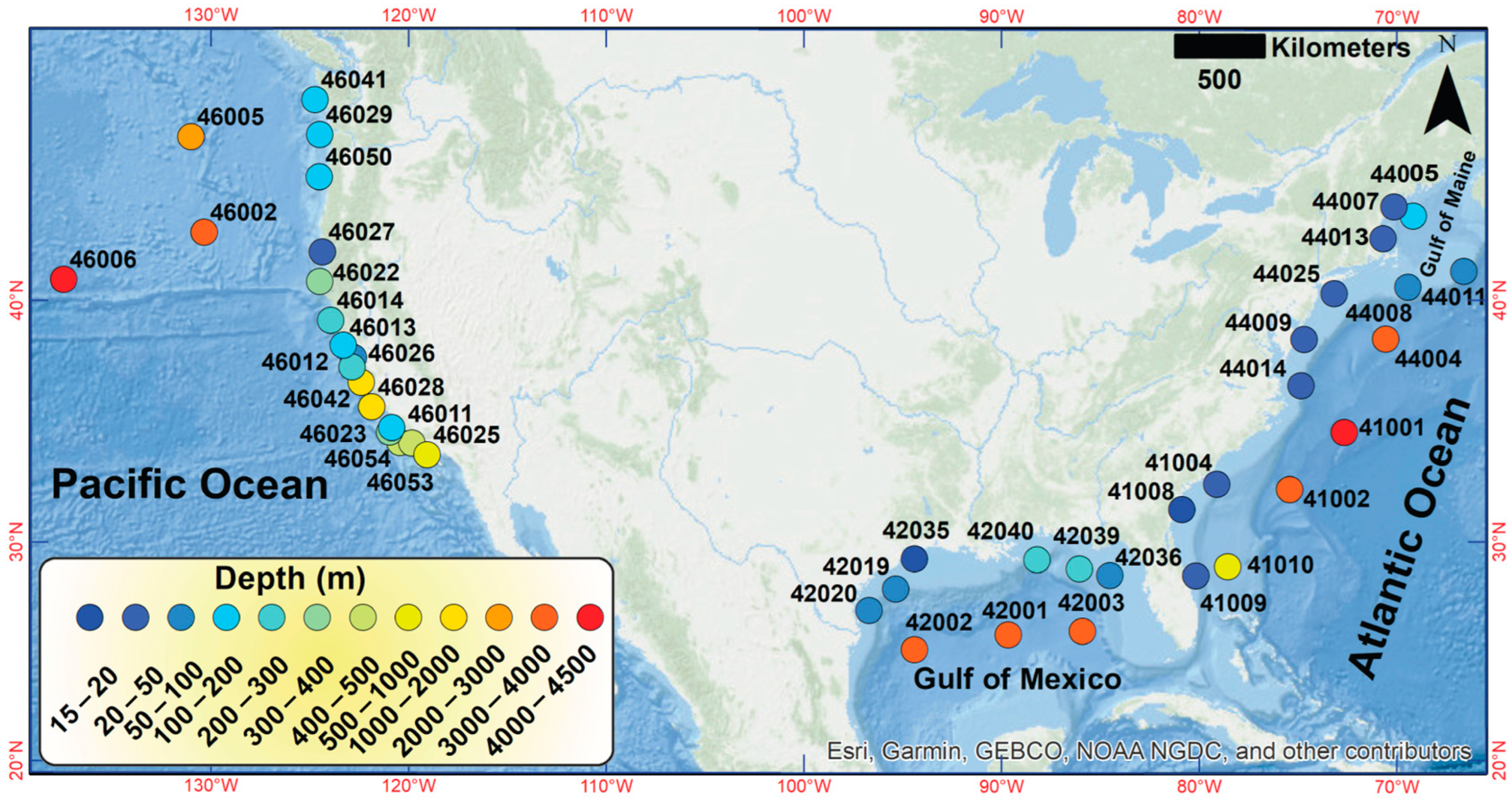
2.1. Data and Preprocessing

The raw data we considered in this study are SWH measurements obtained from the NDBC buoys. We only consider buoys that have at least 20 years of SWH records between 1990 and 2020, given that wave climate studies need a long-term record of data. Based on this criterion, Figure 1 shows the selected 43 buoys off the U.S. Pacific, Atlantic, and Gulf of Mexico Coasts. Most buoys are located on continental shelves. The shallowest buoy station, buoy 42035, is located at a water depth of 16.2 m in the Gulf of Mexico. The water depth is deepest (4486 m) at the location of buoy 41001 in the Atlantic Ocean.

The measured wave data are analyzed to investigate the monthly and seasonal variability and trend in the mean and extreme SWH, and the number of extreme wave events. We use the 95th percentile SWH as a proxy for the extreme SWH. The seasonal analysis is performed for a cold season extending from October to April and a warm season from May to September. Most buoy measurements are available at an hourly time step. At a few buoy stations, measurements are at time intervals other than hourly, e.g., every three hours or every 30 min. For the analyses described later, it is desirable to compile time series with a constant sampling time step. Therefore, using linear interpolation, we first reconstruct the hourly time series for time periods where measurements show unequal sampling frequencies. The quality of the interpolated time series is checked to assure that the statistical characteristics of the original data are preserved. This is performed through qualitative comparisons using histograms and scatter plots, and quantitative metrics such as the residual sum of squares. All buoys showed no noticeable differences between the original and interpolated time series. An example of this preprocessing is shown for buoy 46005 in Supplementary Figure S1. Due to the interpolation, which resulted in an increased number of data points, the histogram has shown a change in the counts (vertical shifting), yet no change in the statistical characteristics of the data (horizontal shifting) was noticed.

We perform monthly and seasonal variability and trend analyses using only months and seasons that contain an adequate amount of data. The percentage ratio of available hourly readings in the SWH record to the total number of hours in a given month or season serves as a measure of data availability in that month or season. In the literature, the percentage of data availability above which a set of data can be used for analysis is a subject of debate. For monthly time series, refs. [20,21] omitted months with data availability smaller than 40 percent. For their seasonal analysis, refs. [29,30] omitted a whole season if any month in that season had less than 40 percent data availability. Ref. [31], on the other hand, implemented a more stringent criterion in their winter wave analysis, by omitting winter seasons with data availability below 80 percent. In the present study, for monthly data analysis, we adopt the [20,21] approach, which removes any month with data availability below 40 percent. Similarly, for our seasonal analysis, we only include seasons whose data availability is at least 40 percent and have at most one month with data availability of less than 40 percent.

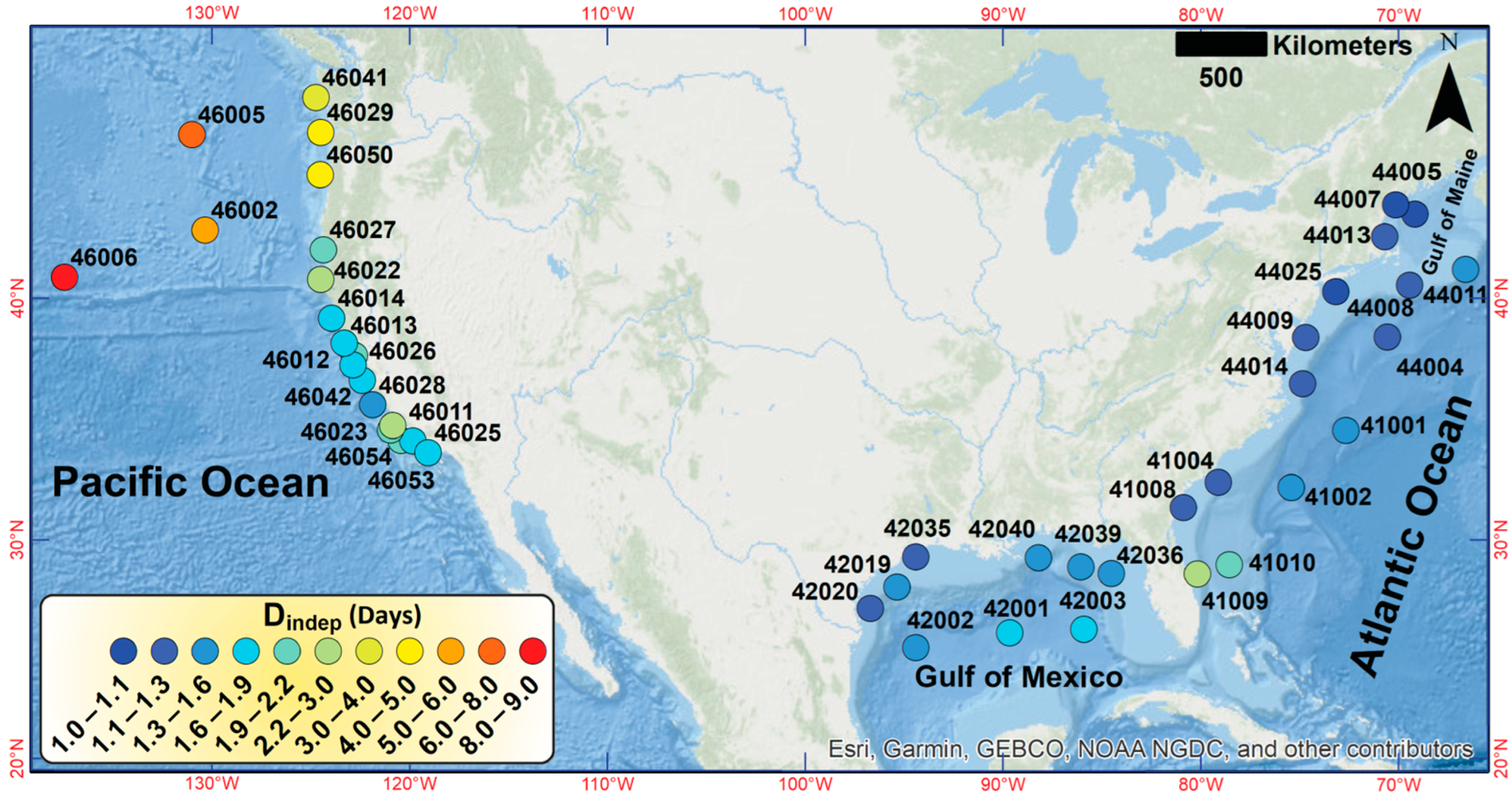
2.2. Extreme Wave Event Detection

Extreme wave events can be defined as waves with a height above a threshold such as a percentile (e.g., 95th, 99th) of the entire wave height record. To identify extreme events, a widely used method is the peaks-over-threshold (POT) method implemented by [20,21,32,33,34,35]. The POT method identifies extreme wave events based on two parameters, including an extreme wave height threshold (hereafter $H_{thresh}$) and a timespan between independent consecutive extreme events (hereafter $D_{indep}$). In this method, an extreme wave height is any SWH that exceeds $H_{thresh}$. Hence, an extreme wave event is a continuous time series of extreme wave heights that last for a sufficiently long time. In this study, we use the minimum length of an extreme wave event to be longer than three hours, making sure that the selected event is not a noise in the wave record. An extreme wave event ends when SWH becomes smaller than $H_{thresh}$ for a duration longer than $D_{indep}$.

There is no general rule for the selection of $H_{thresh}$ and $D_{indep}$. The selection of these parameters for a particular region is subject to the expert’s choice. Choosing $H_{thresh}$ is a double-edged problem since the threshold needs to be as low as possible such that all extreme events are properly identified without bias and to be as high as possible to capture actual extreme events but not too high that it captures a small number of events. Refs. [36,37] considered the 90th percentile as the threshold of extreme wave events, while [10,38] considered the 90th and 99th percentiles as extreme waves. Refs. [39,40,41] used the 95th percentile for their extreme value analyses. In this study, we set $H_{thresh}$ to the 95th percentile of hourly SWH measurements at each buoy. For any month in the warm season, extreme wave heights are identified as wave heights larger than the warm-season threshold, which represents the 95th percentile of all warm-season hourly SWH measurements. Similarly, a cold-season threshold is used to identify extreme wave heights in the cold season.

Many approaches have been proposed to choose $D_{indep}$, which resulted in a wide range of values from 1.25 to 20 days for different ocean basins [20]. The approach proposed by [42,43] was based on the analysis of atmospheric patterns to obtain the length of storms. Their results present the spatial variation in the length of the storms, with a Northeast Pacific duration of 11 days. Another approach, which is adopted in the present study, accounts for a geographic- and climate-dependent $D_{indep}$ through an autocorrelation function (ACF). In this approach, $D_{indep}$ should be longer than the time interval between the local maxima in the time series. This can be achieved by choosing $D_{indep}$ to be longer than the time lag corresponding to an ACF of between 0.3 and 0.5 [44]. The ACF, r_k, can be estimated as per [45].

$$r_k=\frac{c_k}{c_0}$$

where $c_k$ is the estimated autocovariance of the SWH hourly time series calculated as

$${\mathrm{c}}_{\mathrm{k}}=\frac{1}{\mathrm{n}}{\displaystyle \sum }_{\mathrm{t}=1}^{\mathrm{n}-\mathrm{k}}\left({\mathrm{SWH}}_{\mathrm{t}}-\overline{\mathrm{SWH}}\right)\left({\mathrm{SWH}}_{\mathrm{t}+\mathrm{k}}-\overline{\mathrm{SWH}}\right) \mathrm{k}=0, 1, 2, \dots , \mathrm{K}$$

In addition, $c_0$ is the variance, the overbar sign represents the mean, n is the number of readings, and t is the time step between readings. Since we are considering hourly data, n is the number of hours in a certain year and K is equal to n − 1. K determines what time lags are considered for the analysis (K$<$n). We set $D_{indep}$ to the smallest time lag corresponding to an ACF of 0.4 (i.e., the average of the recommended AFC range 0.3–0.5).

For each buoy station, we calculate a representative $D_{indep}$ by averaging the values of $D_{indep}$ that are separately calculated from each year. Only years with data availability of 95 percent or higher are considered, given that continuous time series with equal sampling steps are desirable for the autocorrelation approach. Figure S2 shows an example of the correlogram between the ACF and the time lag for the buoy station 46027. At this station, an ACF of 0.4 is obtained within 2.3 days in most years. The average $D_{indep}$ for each buoy station is shown in Figure 2. Overall, stations in the Pacific Ocean show a longer timespan between consecutive extreme wave events than stations in the Atlantic and Gulf regions. In the Pacific, $D_{indep}$ is between 1.9 and 8.8 days, with the largest values calculated for buoys at higher latitudes. In the Atlantic and Gulf, $D_{indep}$ is typically smaller than 1.5 days but is between 1.5 and 2.3 days in a few low-latitude stations. We use the estimated $D_{indep}$, together with the wave height thresholds described earlier ($H_{thresh}$), to identify extreme wave events from the SWH hourly time series.

2.3. Trend and Variability Metrics

We calculate the monthly, seasonal, and interannual variabilities and trends in the mean and 95th percentile SWHs and the number of extreme wave events. Trends are calculated using ordinary least squares regression for the long-term period of 1990–2020 as well as for every decade since 1980. The long-term trends are only calculated for buoys that have at least twenty years of data. Decadal trends are calculated for decades that have at least seven years of data in that decade. The coefficient of variance (CV), which is the ratio of the standard deviation to the mean value, is used to measure monthly and interannual changes in time. The variability analysis is performed on the linearly detrended time series to remove the effects of climate change. The quantified trends and variabilities across the buoy stations are presented and discussed in the following section.

3. Results and Discussion

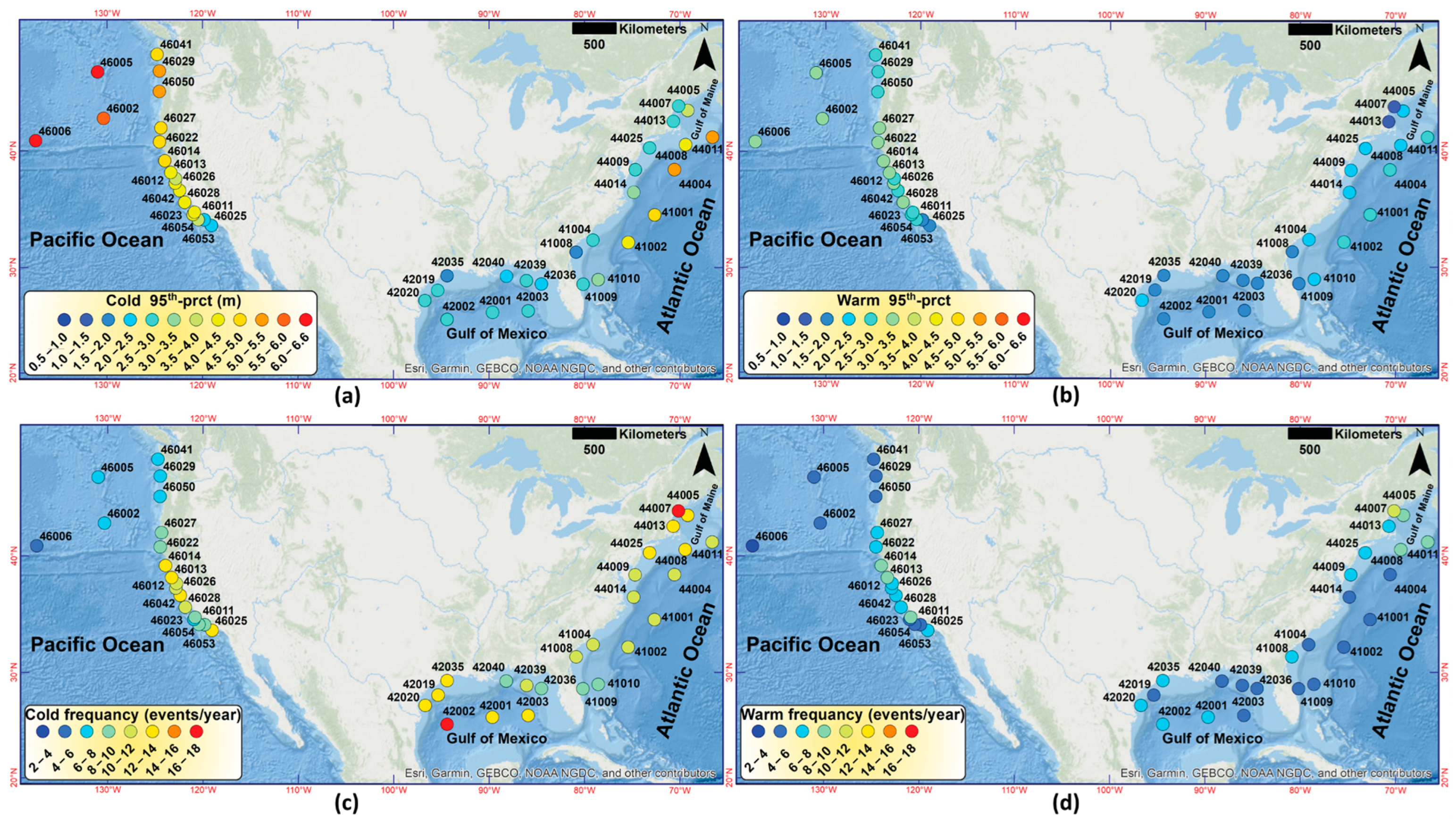
3.1. Extreme Wave Climate

The seasonal 95th percentile SWH, i.e., $H_{thersh}$, for the cold and warm seasons from 1990 to 2020 is presented in Figure 3a,b, respectively. The cold-season 95th percentile SWHs at buoys in the northern part of the Pacific are larger than those in the southern part, with the largest 95th percentile SWH being 6.4 m at buoy 46006. This is because, during the cold season, buoys at higher latitudes are exposed, at a higher level, to storms generated in the Bearing Sea and Gulf of Alaska regions due to the low-pressure system located near the Aleutian Islands. The smallest 95th percentile SWH (1.5 m) is calculated for the warm season at buoy 44013 in the Gulf of Maine. Small warm-season 95th percentile SWHs are also found for buoys across the Gulf of Mexico.

In the Pacific region, both cold- and warm-season numbers of extreme wave events at lower latitudes are larger than those at higher latitudes. This is due to the smaller $H_{thresh}$ at lower-latitude buoys (see panels Figure 3a,b), resulting in southern swell events being identified as anomalies and, thus, more often considered extreme events. Buoys at lower latitudes experience swells from different sources, with the main source of swells traveling from the Southern Hemisphere to the Northeast Pacific region [46]. In addition to swells from the Pacific basin, buoys at lower latitudes of the Eastern North Pacific are exposed to swells that originate from the extratropical areas of the Eastern South Indian Ocean (ETSI) and Southwestern Pacific Ocean [47]. High-intensity extreme wind events in the ETSI basin occur during cold- and warm-season [48], resulting in large swells reaching the Eastern North Pacific region and contributing to the number of extreme wave events in the region. In addition to swells originating in the ETSI, swell waves generated by tropical cyclones (TCs) in the Eastern North Pacific contribute to the larger number of extreme wave events at low-latitude buoys off the U.S. West Coast.

Buoys in the Atlantic Ocean experience an opposite spatial pattern in the number of extreme wave events. Both the cold- and warm-season numbers of extreme wave events at higher latitudes are larger than those at lower latitudes. In the cold season, this is attributed to the effects of extra-tropical cyclones (ETCs) in the extratropical North Atlantic areas. Track densities of historical ETCs [49,50] show that a larger number of ETCs is concentrated above a latitude of 40 °N. In the summer, swell events generated by the Southern Hemisphere’s winter storms in the extratropical South Atlantic areas can reach high latitudes above 35 °N [47], while lower-latitude areas are sheltered from the swells.

In the Gulf region, the cold- and warm-season numbers of extreme wave events are larger at buoys across the west side of the Gulf. This is consistent with the results from [51], who showed that the mean SWH on the western side of the Gulf is larger than that on the eastern side. In the cold season, wave climate in the Gulf is influenced by anticyclonic cold fronts. Among the five types of cold fronts in the Gulf of Mexico, types 2–5 exert the most influence on the wave climate of the Western Gulf region, with types 2 and 3 generating the most energetic waves [52]. The influence of cold fronts on extreme events is limited to the cold season, given that these storms dominate between October and April [52,53]. In the warm season, the number of extreme events in the Gulf is influenced by hurricanes in the Gulf of Mexico and the Western Caribbean Sea, generating wind waves that travel northwest through the Yucatán Channel and the Western Gulf of Mexico. On average, eight hurricanes per year pass across or near the Caribbean during the Atlantic hurricane season [54]. The number of extreme wave events in the Gulf region is also affected by the Caribbean Low-Level Jet (CLLJ) [52], i.e., easterly zonal wind at 925 hPa in the Caribbean region [55]. The CLLJ intensifies in February during the cold season and in July during the warm season, generating extreme waves that can reach the western part of the Gulf of Mexico through the Yucatán Channel.

Figure 3. Long-term (1990–2020) 95th percentile SWH ($H_{thesh}$) for (a) cold and (b) warm seasons and long-term frequency of extreme wave events for (c) cold and (d) warm seasons.

Figure 3. Long-term (1990–2020) 95th percentile SWH ($H_{thesh}$) for (a) cold and (b) warm seasons and long-term frequency of extreme wave events for (c) cold and (d) warm seasons.

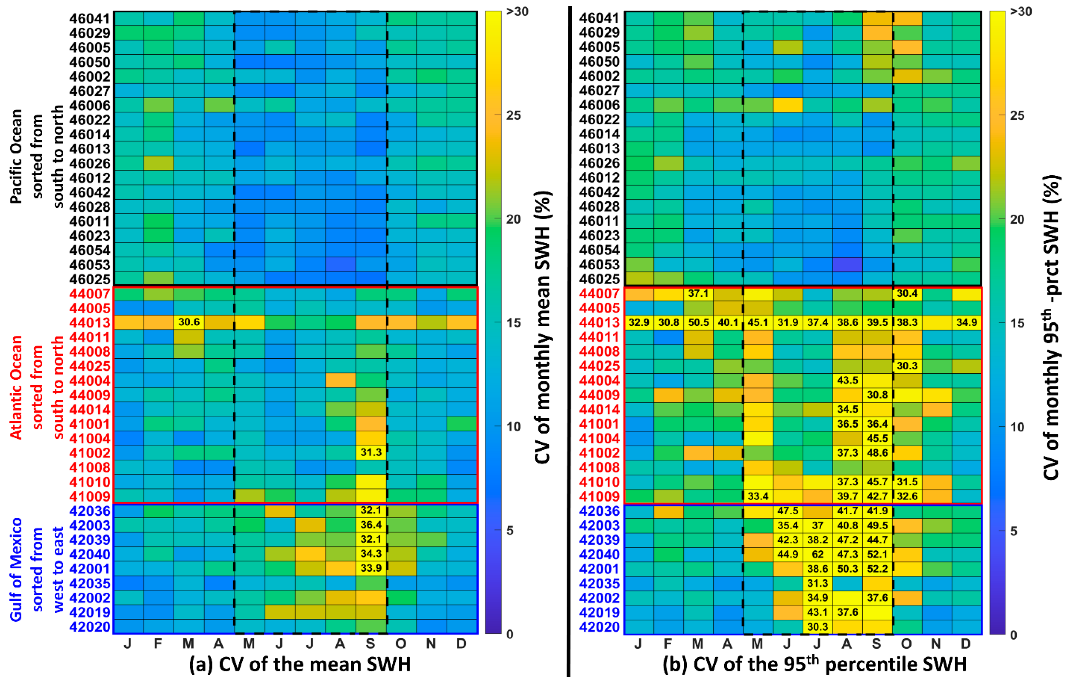
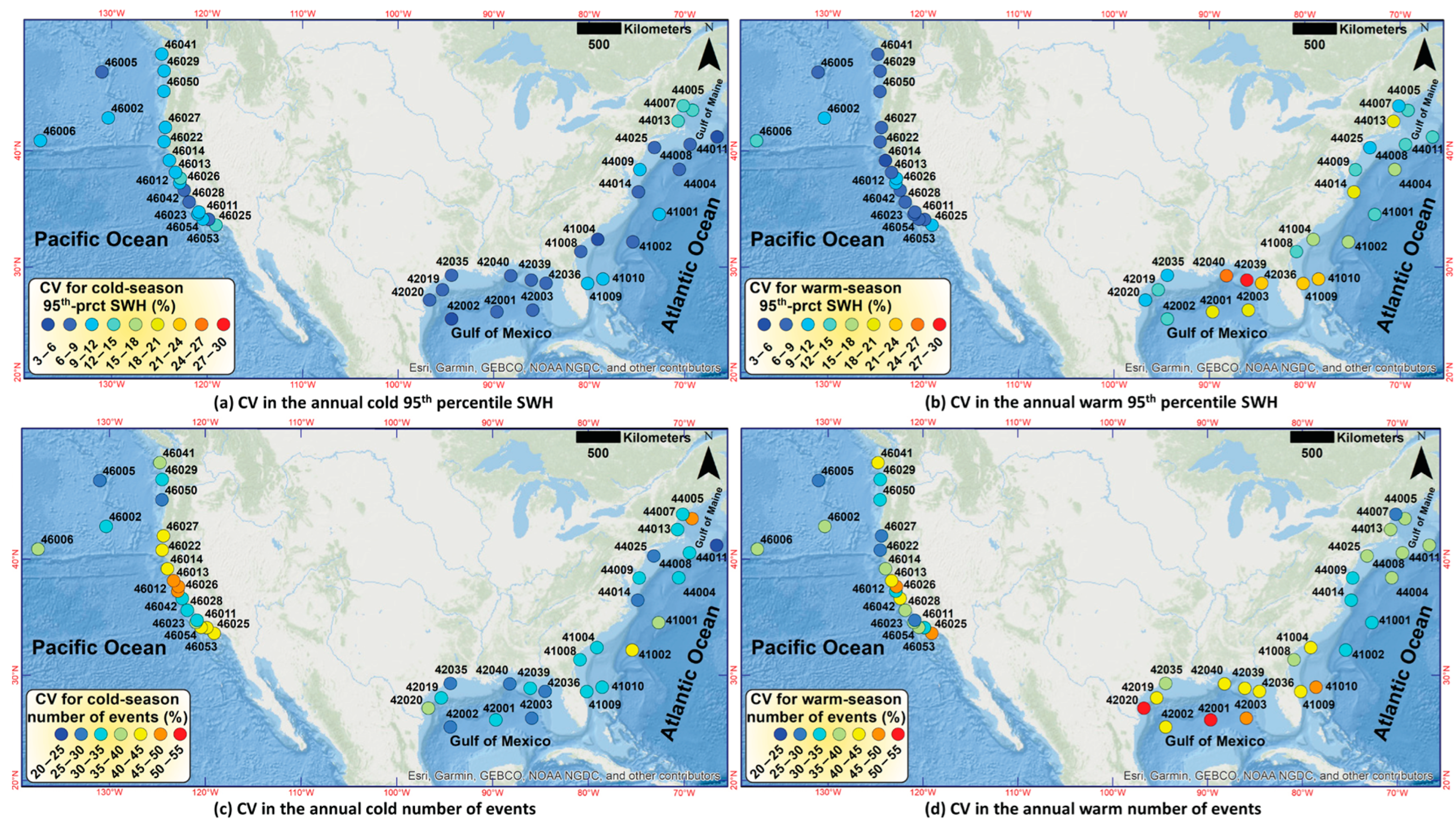
3.2. Seasonal and Interannual Variabilities

Figure 4 shows the calculated CVs for the monthly mean and 95th percentile SWH. Overall, in warm-season months, the interannual variabilities across the Gulf and Atlantic regions are larger than those across the Pacific. The largest variabilities are observed in the Gulf and Southern Atlantic regions, especially for the 95th percentile of the SWH. Buoys in these regions are exposed to waves generated by TCs during the Atlantic hurricane season (June–November). Therefore, the year-to-year variation in the frequency and intensity of TCs in the Atlantic basin influences the wave climate variability. In the Pacific region, interannual variabilities in the monthly mean and 95th percentile SWH during the cold season are larger than those during the warm season. In contrast to buoys in the Pacific, the variability in SWH across the Gulf and Atlantic regions is larger during the warm season than during the cold season.

In addition to meteorological factors, wave climate variability can be influenced by other factors such as water depth and land masses. At buoy 44013, located at a water depth of 65 m in the Gulf of Maine, large interannual variabilities are observed in the mean and 95th percentile SWH of every month, regardless of the season. This is also the case for buoy 44007, which is located at a water depth of 49 m in the Gulf of Maine. Smaller variabilities are observed at buoy 44005, which is in the same region but at a deeper water depth (i.e., 177 m). The larger variabilities in the SWHs at buoys 44013 and 44007 can be attributed to multiple reasons, such as the small wind fetch and shallow waters. In specific, the wind fetch at buoy 44013 is limited by landmasses in the south, east, and north of the buoy. In addition, the longest fetches are associated with easterlies and south easterlies. Therefore, any variability in the wind direction can lead to a substantial change in the variability of wave heights at this buoy. Another reason for high interannual variabilities at buoys 44007 and 44013 can be because of the effects of tides and tidal currents in shallow waters, given that the tidal range in the Gulf of Maine is large. For example, the mean range of the tide is 2.9 m at the Boston tide gauge to the west of buoy 44013. Given that wave events can coincide with any tidal phase, this randomness in the arrival time of waves can result in a larger variability in the seabed-wave-current interactions and, potentially, the wave heights.

Figure 4. Coefficient of variation (CV) for the interannual variability in the monthly mean and 95th percentile SWHs. Numbers represent CVs greater than 30 percent. The dashed lines confine the warm season.

Figure 4. Coefficient of variation (CV) for the interannual variability in the monthly mean and 95th percentile SWHs. Numbers represent CVs greater than 30 percent. The dashed lines confine the warm season.

We examine the coefficient of variation for the variability in the annual cold- and warm-season 95th percentile SWHs (Figure 5a,b) and the number of extreme events (Figure 5c,d). In the Pacific, interannual variabilities in the cold-season 95th percentile SWH are nearly equal or slightly larger than those in the warm-season SWH. There is a slight spatial variability in the calculated CV across the Pacific region, yet the CV remains below 15% at most buoys. Similar to the Pacific region, the cold-season CV calculated for buoys in the Gulf and Atlantic regions is smaller than 10%, except for high-latitude buoys in the Gulf of Maine, where CV reaches up to 15%. However, in the warm season, the interannual variabilities in the 95th percentile SWH in the Gulf and Atlantic regions are larger than those in the Pacific, with CV reaching up to 30% in the Gulf region. The largest variabilities are calculated for the warm-season 95th percentile SWH at buoys in the eastern region of the Gulf of Mexico. Although this region is sheltered from swells generated in the Atlantic Ocean, it is located within the Atlantic Hurricane Alley, which makes the warm-season wave climate in this region correlate to the year-to-year variability in the number and intensity of TCs.

The interannual variability in the number of extreme wave events in the warm season is larger than that in the cold season. For the cold-season number of extreme wave events in the Pacific, smaller variabilities are calculated for buoys at a higher latitude. In the Atlantic and Gulf regions, the CV in the cold-season number of events at most buoys is between 20% and 40%, without any specific spatial patterns. For the warm season, the CV in the seasonal number of events is larger in the Gulf region than in other regions. In the Atlantic, an increasing spatial trend (22–55%) from north to south is observed.

Figure 5. Coefficient of variation (CV) for the interannual variability in the annual cold- and warm-season 95th percentile SWHs (a,b) and the annual number of extreme wave events (c,d).

Figure 5. Coefficient of variation (CV) for the interannual variability in the annual cold- and warm-season 95th percentile SWHs (a,b) and the annual number of extreme wave events (c,d).

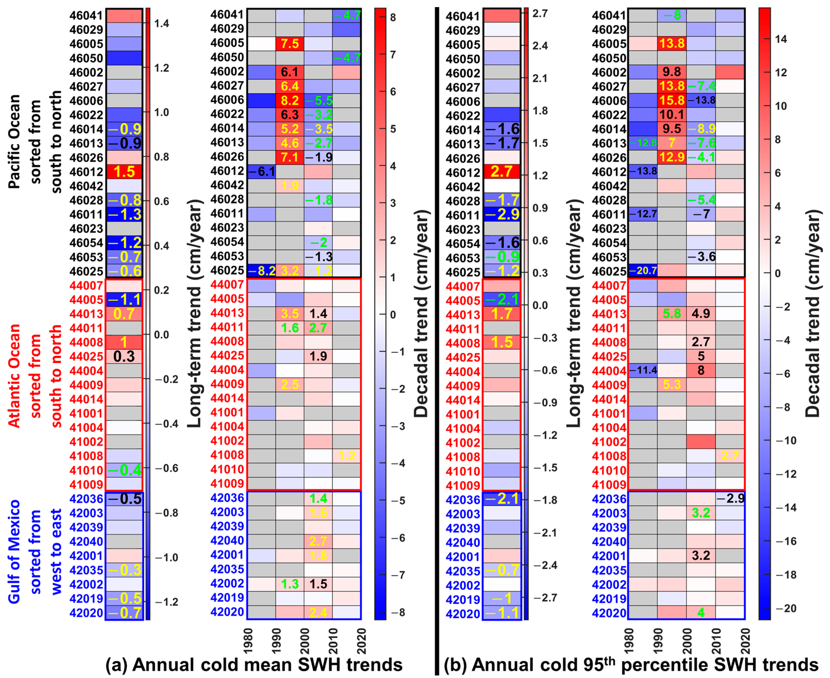
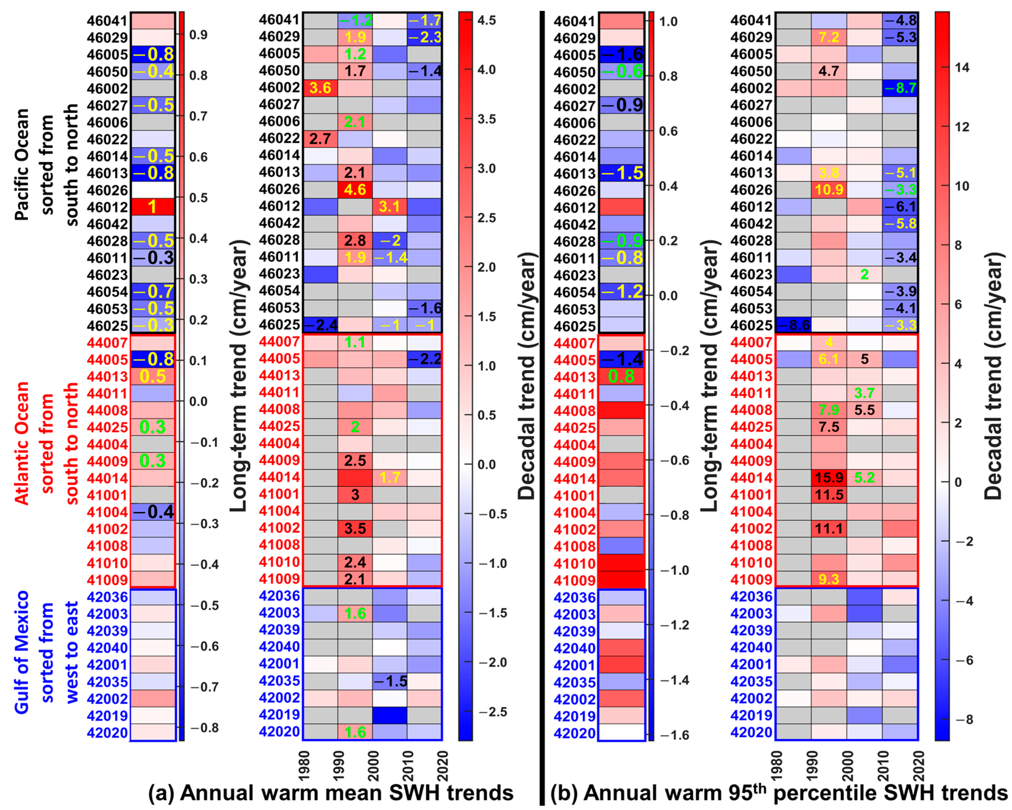
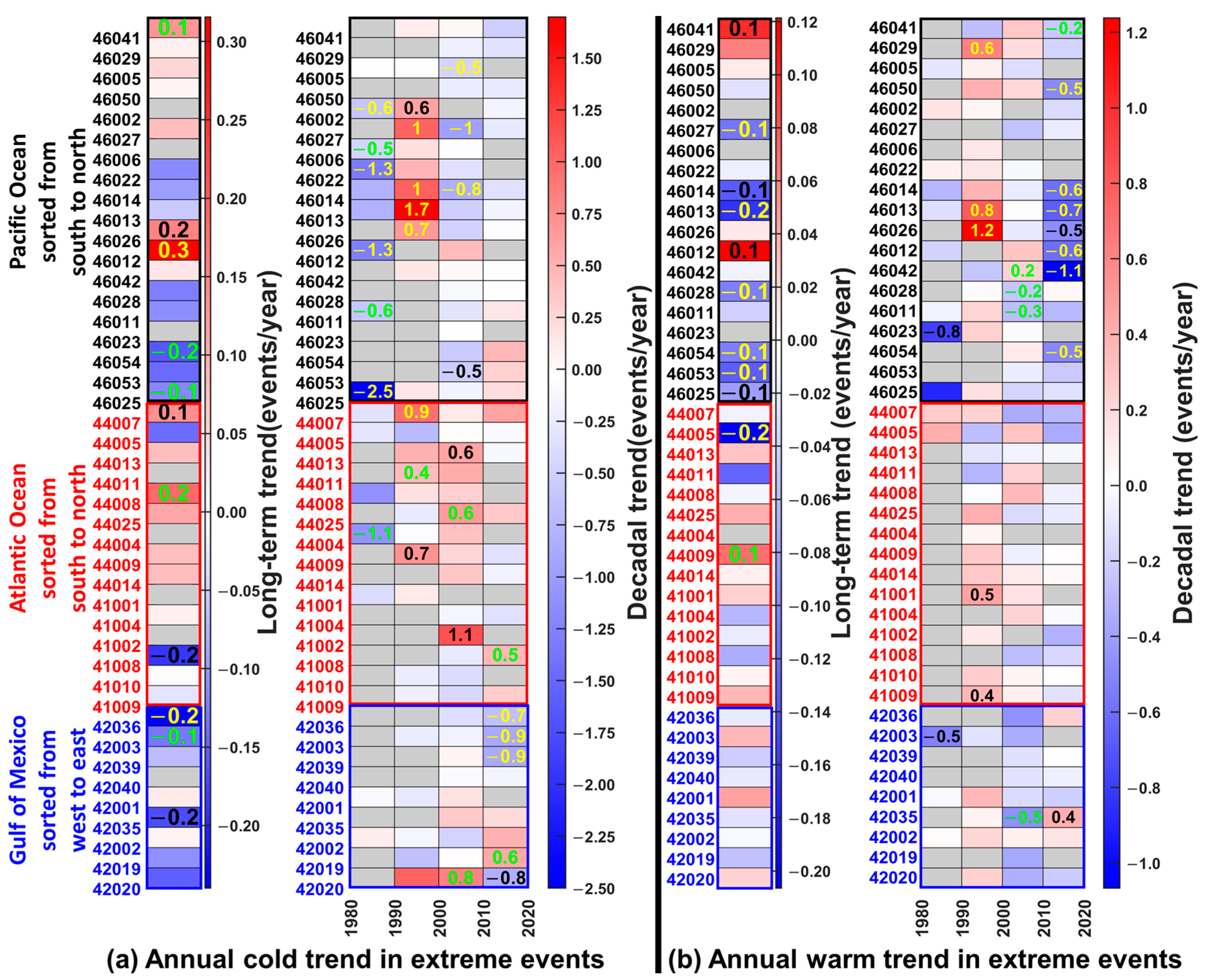
3.3. Decadal and Long-Term Trends

In this section, we present and discuss linear trends in the mean and extreme wave heights and the number of extreme events. The trend analysis was applied on a long-term and decadal basis. While a long-term trend is useful for identifying the long-term changes in the wave climate, it does not provide insight into the non-stationarity of the wave climate change (e.g., decadal changes in trends). In the following sections, for each region, we first describe the long-term (1990–2020) and decadal trends in the cold- and warm-season mean and extreme wave climate, and the number of extreme events. Since one of the scopes of this study is to investigate the effects of including the last decade in trend analysis, we compare our results with existing studies that did not include the measurements from the last decade in their analyses. We further discuss the connection between the long-term and decadal wave height trends and the large-scale climate.

3.3.1. Pacific Ocean

• Cold Season

The calculated long-term trends (single column in Figure 6a,b) in cold-season SWH at most buoys across the Pacific show a negative trend between −0.6 and −1.3 cm/yr in the mean SWH and between −0.9 and −2.9 cm/yr in the 95th percentile SWH. In general, the aforementioned trends are statistically significant, at a 95% confidence level, at buoys located at lower latitudes. Out of 15 buoys in the Pacific, only three of them are characterized by a positive long-term trend in the cold-season SWH, with significant trends of 1.5 and 2.7 cm/yr, respectively, in the mean and 95th percentile SWH at buoy 46012.

The Pacific buoy stations show very strong positive decadal trends during the 1990s, ranging from 1.9 to 8.2 cm/yr for the mean SWH (multiple columns in Figure 6a) and between 7 and 15.8 cm/yr for the 95th percentile SWH (multiple columns in Figure 6b). The only negative trend in the 1990s is calculated at buoy 46041, the northmost buoy. These strong trends dominate the northern part of the Pacific region. The strong positive trends in the 1990s are followed by strong negative trends in the following decade. In the 2000s, the largest negative trends are calculated at buoy 46006, with a trend of −5.5 cm/yr in the mean SWH and −13.8 cm/yr in the 95th percentile SWH.

Overall, the long-term trends in the number of cold-season extreme events (single column in Figure 8a) are positive but not significant at high-latitude buoys in the Pacific. At the lower latitudes, trends are generally negative, except for buoys 46042, 46012, and 46026. The largest positive trend, which is also statistically significant, is found for buoy 46012 (0.3 events/yr). Similar to decadal trends in SWH, the decadal trends in the number of extreme wave events (multiple columns in Figure 8a) do not necessarily agree with the long-term trends. Significant positive trends were observed at multiple buoys during the 1990s. This is consistent with the very strong positive trends in SWH during the same decade. The strong positive trends of the 1990s were followed by negative trends in the 2000s. Trends during the last decade show nonsignificant changes in all buoys in the Pacific region.

• Warm Season

The long-term trends in the warm-season SWH show significant negative trends at most buoy stations (Figure 7a,b). However, positive trends are calculated for buoy 46012 and the northmost buoys 46029 and 46041. The largest negative trends are calculated at buoys 46005, 46013, and 46054 and are between −0.7 and −0.8 cm/yr for the mean SWH and between −1.2 and −1.6 cm/yr for the 95th percentile SWH.

Similar to the trends in cold-season SWH presented earlier, the warm-season mean (Figure 7a) and 95th percentile (Figure 7b) SWHs show positive trends in the 1990s, which contrast the negative long-term trends. The increasing wave heights in the 1990s were followed by two decades of decreasing wave heights, as shown by negative trends in the 2000s and 2010s. The strongest significant negative trends are calculated for the 2010s, in which the trends in the mean and 95th percentile SWH reached −2.3 and −8.7 cm/yr, respectively.

Long-term trends in the number of extreme wave events for the warm season generally show a spatial pattern similar to those for the cold season, i.e., positive trends in northern buoys and negative trends in southern buoys, except for buoys 46012 and 46026. However, the increasing trends calculated for the warm season are smaller than that for the cold season. Similar to the cold-season decadal trends, the decadal trends in the number of warm-season extreme wave events were positive in the 1990s. The decadal trends show a decreasing number of extreme wave events during the most recent decade (i.e., the 2010s). The 2010s negative trends are statistically significant in many buoy stations, with the largest calculated trend being −1.1 events/yr at buoy 46042. This contrasts with the 2010s cold-season trends, which showed non-significant changes in the number of extreme wave events in the Pacific.

Our trend analysis using buoy data for the period of 1990–2020 showed a negative trend in the mean SWHs, which reached up to −1.3 cm/yr in the cold season and −0.8 cm/yr in the warm season. This is consistent with the decreasing trends found by [11] for the period of 1985 to 2018. However, our calculated negative trends in most buoys have discrepancies with [36], who found increasing trends. This is due to the effects of the 2010s trend, which were not included in [36]. Our calculated decadal trends for the 2010s clearly show a decreasing trend in the mean SWH, especially for the warm season. These negative decadal trends of the 2010s have an important impact on the estimated long-term trends. Furthermore, not including the 1980s decade, our calculated 1990–2020 trend for buoy 46005 showed a statistically non-significant decreasing trend compared to the statically significant trend of 2.3 cm/yr for the period 1975–2007 calculated by [29] for the same buoy. Our estimated decadal trends for the 1980s show a small and non-significant trend of 0.1 cm/yr followed by a strong trend of 7.5 cm/yr in the 1990s, reiterating the importance of the time span of the data used in wave climate analyses and the consideration of wave climate non-stationarity.

• Links to Global Climate and Regional Effects

In the Eastern North Pacific Ocean, the wave climate is correlated with the El Niño-Southern Oscillation (ENSO) and Southern Annular Mode (SAM) [21,56,57]. During El Niño events (+0.5 °C SST anomaly in the NINO3.4 region), the northern jet stream intensifies and shifts southward, resulting in an equatorward shift in the storm tracks of the North Pacific [58]. This results in the southern region of California experiencing increased wave activity during El Niño episodes [59]. In contrast, the northern region has a greater number of winter storms and increased wave activity during La Niña episodes, due to the poleward shift of storm tracks. We found that the detected positive trends in the cold-season SWH during the 1990s coincide with the negative trend in the NINO3.4 index (Figure S3), a trend toward La Niña episodes. In the first two decades of the 21st century, the negative decadal trends in SWH at higher-latitude buoys coincide with the positive trend in the NINO3.4 index, which indicates a trend toward El Niño and, thus, decreased wave activities in the northern regions. The wave climate in the Northern Hemisphere is also influenced by waves generated in the Southern Hemisphere, especially during austral winters. This is illustrated by the correlation between the SAM index and the wave energy at a region from the Eastern South Pacific to mid-latitude regions of the Eastern North Pacific [57]. Thus, the variability in the SAM, which is associated with the north–south movement of the westerly wind belt surrounding Antarctica, could influence the calculated trends in the SWH. Our calculated positive trends in warm-season SWH in the 1990s coincide with the positive trend in the SAM between 1990 and 2000 (Figure S4), as also shown by [14]. In contrast, the significant negative trends in SWH in the 2010s coincide with the negative trend in the SAM during this decade.

3.3.2. Atlantic

• Cold Season

In the northern areas of the Atlantic region, the long-term cold-season trends are positive for most buoys. One of the largest statistically significant positive trends is calculated at buoy 44013, located in the Gulf of Maine. At this buoy, positive trends of 0.7 cm/yr in the mean SWH and 1.7 cm/yr in the 95th percentile SWH are calculated. A negative trend in the northern areas of the Atlantic region is calculated only at buoy 44005, which shows a significant decrease of −1.1 cm/yr in the mean SWH and −2.1 cm/yr in the 95th percentile SWH. In the southern area of the Atlantic region, the calculated trends are negative but not statistically significant. The trend of −0.4 cm/yr in the mean SWH at buoy 41004 is significant only at an 85% confidence level.

Atlantic decadal trends at most buoys do not show any significant departure from the long-term trends. At buoys in lower latitudes of the Atlantic region, similar to the long-term trends, the decadal trends show a decrease in SWH. At buoys in the higher-latitude areas, the decadal trends do not necessarily agree with the long-term trends. For instance, at buoys 44013 and 44009, while the long-term trend is positive, the decadal trend in the 2010s shows a negative trend, although it is not significant.

We found nonsignificant positive and negative long-term trends in the cold-season number of extreme wave events. Negative trends are calculated in the southern areas of the Atlantic region. The largest decrease is −0.2 events/yr at buoy 41008. For buoys at higher latitudes, positive trends are found at most buoys except buoy 44005, where a decrease of −0.1 events/yr is found. The decadal trends of the number of extreme cold events show a generally increasing trend in all decades except the 1980s.

• Warm Season

The long-term trends show both negative and positive trends in the warm-season mean and 95th percentile SWHs. The largest significant positive trend is calculated for buoy 44013 in the Gulf of Maine, where the trends are 0.5 and 0.8 cm/yr for the mean and 95th percentile SWHs, respectively. Similarly, the largest significant negative trend is calculated in the Gulf of Maine, at buoy 44005 where the mean and 95th percentile SWH have decreased, respectively, by −0.8 and −1.4 cm/yr from 1990 to 2020.

Our analysis shows generally positive decadal trends in the 1990s and 2000s for the mean and 95th percentile SWH. The largest positive trends are calculated for the 1990s, a decade in which the calculated increases in the mean and 95th percentile SWHs are statistically significant at many buoy stations. For example, we find positive trends of between 1.1 and 3.5 cm/yr in the mean SWH. In the 2000s, while trends are positive, they are smaller compared to the 1990s. In the 2010s, both negative and positive trends were calculated, but they were not significant.

The warm season’s long-term annual number of extreme wave events between 1990 and 2020 shows a significant change at only two buoys. We find a significant decreasing trend of 0.2 events/yr at buoy 44005 and an increasing trend of 0.1 events/yr at buoy 44009. However, decadal trends calculated for these buoys do not show a significant change in any of the past three decades. Decadal trends calculated for the 1990s and 2000s show both negative and positive trends, depending on the region. In the 2010s, the estimated trends are generally negative or near zero.

• Links to Global Climate and Regional Effects

The results presented above showed negative trends in the SWHs and the number of extreme wave events at buoy 44005 in the Gulf of Maine, whereas the calculated trend at buoy 44013 in the same region is positive. In addition to the local weather conditions, additional factors influence the wave climate at this buoy compared to 44005. For instance, Cape Cod shelters buoy 44013 from Atlantic swells that travel from the south to the Gulf of Maine. In contrast, buoy 44005 is exposed to swells from the south. Another factor associated with the wind fetch is that the limited fetch can minimize the effects of specific weather patterns on the local wave climate. For example, the wind fetch of southerlies at buoy 44013 is limited, whereas the wind fetch at buoy 44005 extends to the Atlantic Ocean. This reiterates the importance of other factors such as landmasses on the wave climate. Future research is needed to better understand factors that influence the spatial variability of the wind wave climate in the Gulf of Maine.

The results show strong positive trends in the warm-season SWH in the 1990s, a decade with an increasing number of hurricanes. This is consistent with the recorded number of days with hurricanes in the Atlantic Ocean, as it shows a positive trend of 3.26 days/yr in the 1990s (Figure S5). Trends in cold-season SWH at most buoys at high latitudes were positive in the 2000s but negative or showed nearly no change in the 2010s. In the cold season, the buoys at high latitudes are influenced mainly by extratropical cyclones in the North Atlantic. The frequency and intensity of these cyclones are correlated with the large-scale atmospheric circulation, which can be described by the North Atlantic Oscillation (NAO) climate index [60]. The NAO index, which is determined based on the pressure difference between the Subtropical (Azores) High and the Subpolar Low, indicates changes in the intensity and location of the North Atlantic jet stream and storm tracks. A negative phase of the NAO represents a decreased pressure gradient, resulting in weaker westerly winds and smaller waves across Western Europe [61]. In Eastern North America, the negative phase of the NAO generally results in stronger cold-air outbreaks and increased storminess. This implies that the positive trends in SWH during the 1990s and 2000s are attributed to decreasing trends in the NAO index (Figure S6) and, thus, increased storminess during these two decades. In contrast, a positive phase of the NAO results in stronger westerlies and, thus, decreased storminess in Eastern North America. The detected slightly decreasing trends in SWH between 2010 and 2020 coincides with the positive trend in the NAO index during the 2010s.

3.3.3. Gulf of Mexico

• Cold season

Across the Gulf region, the long-term trends are generally negative in the cold season. Buoys on the western side of the Gulf, i.e., buoys 42020, 42019, and 42035 experience significant decreasing trends. The only positive trends, although nonsignificant, are 0.2 and 0.5 cm/yr in the mean and 95th percentile SWH, respectively, at buoy 42001. In contrast to the negative long-term trends, our analysis shows positive decadal trends for the 1990s and 2000s decades. Statistically significant positive trends in the mean SWH are calculated for the 2000s. The 2000s decadal trends in the mean and 95th percentile SWH reach, respectively, 2.7 cm/yr at buoy 42040 and 4 cm/yr at buoy 42020.

Long-term trends in the number of extreme wave events during the cold season are generally negative at most buoys in the Gulf. The trends are statistically significant, at a confidence level of 85% or higher, at three buoy stations 42035, 42003, and 42036. The results show that the decadal trends in the number of extreme events at buoys in the central and western regions of the Gulf alternate between negative and positive. In contrast, at buoys in the eastern part of the Gulf, our results show a negative decadal trend for the past decades. The 2010s decade is associated with the largest negative trends in the number of extreme wave events during the cold season (−0.7 to −0.9 event/yr).

• Warm Season

We find no significant long-term changes in the warm-season mean and 95th percentile SWH in the Gulf region. The calculated trends are between −0.2 and 0.4 cm/yr for the mean SWH and between −0.5 and 0.8 cm/yr for the 95th percentile SWH. The decadal trends show that the 2000s decade was dominated by a negative trend in SWH at all buoys in the region. In contrast to the negative long-term trends in the number of extreme wave events during the cold season, the long-term warm-season trends show nonsignificant spatially scattering negative and positive trends depending on the geographic location of the buoy in the Gulf. Decadal trends in the number of extreme events show negative trends dominating the 2000s.

• Links to Global Climate and Regional Effects

During the warm season, extreme waves in the Gulf region are mainly associated with the passage of tropical cyclones. The decadal trends in SWH at most buoys show a positive trend between 1990 and 2000, which is consistent with the increasing trend (3.26 days per year) in the number of days with hurricanes in the Atlantic Ocean in the 1990s (Figure S5). Similarly, the negative trends in SWH between 2000 and 2010 coincide with the decreasing trend in the number of days with hurricanes in the 2000s (−1.058 days per year).

The detected trends in the cold-season SWH agree with changes in the climatology of anticyclonic cold fronts, which dominate the extreme weather events in the Gulf of Mexico between October and April, a period that coincides with the cold-season duration considered in the present study. Based on observations, the frequency of cold fronts in the Gulf increased between 2002 and 2014 [62]. This implies that our calculated positive trend in the cold-season SWH during the 2000s is consistent with the increasing number of cold fronts in the 2000s.

The results presented above showed negative long-term trends in the cold-season mean and 95th percentile SWH at all buoy stations except at buoy 42001, where a positive trend was observed. This buoy is in the central area of the Gulf, facing the Yucatán Channel, the strait that connects the Gulf of Mexico and the Caribbean Sea. The wave climate at this buoy is directly influenced by the climate of the Caribbean Sea, given that swells that originate in the Caribbean Sea can travel along the great circle routes to pass through the Yucatán Channel and reach the central and northern areas of the Gulf. This is evident in the results obtained by [51] who analyzed a 30-year wave hindcast for the period of 1979–2008 and showed a significant positive trend in the annual mean SWH in the central area of the Gulf of Mexico but nonsignificant trends in the western and eastern side of the Gulf. Their results show larger trends near the Yucatán Channel. Future research can investigate the extent to which swells originating in the Caribbean Sea influence the wave climate change in the Gulf of Mexico.

Figure 6. Long-term (1990–2020) and decadal trends in cold-season (a) mean and (b) 95th percentile SWHs. Cells in gray did not meet the data availability requirements for trend analysis. Numbers in yellow, black, and green represent trends that are statistically significant at 95%, 90%, and 85% confidence levels, respectively.

Figure 6. Long-term (1990–2020) and decadal trends in cold-season (a) mean and (b) 95th percentile SWHs. Cells in gray did not meet the data availability requirements for trend analysis. Numbers in yellow, black, and green represent trends that are statistically significant at 95%, 90%, and 85% confidence levels, respectively.

Figure 7. Long-term (1990–2020) and decadal trends in warm-season (a) mean and (b) 95th percentile SWHs. Cells in gray did not meet the data availability requirements for trend analysis. Numbers in yellow, black, and green represent trends that are statistically significant at 95%, 90%, and 85% confidence levels, respectively.

Figure 7. Long-term (1990–2020) and decadal trends in warm-season (a) mean and (b) 95th percentile SWHs. Cells in gray did not meet the data availability requirements for trend analysis. Numbers in yellow, black, and green represent trends that are statistically significant at 95%, 90%, and 85% confidence levels, respectively.

Figure 8. Long-term (1990–2020) and decadal trends in (a) cold-season and (b) warm-season numbers of extreme wave events. Cells in gray did not meet the data availability requirements for trend analysis. Numbers in yellow, black, and green represent trends that are statistically significant at 95%, 90%, and 85% confidence levels, respectively.

Figure 8. Long-term (1990–2020) and decadal trends in (a) cold-season and (b) warm-season numbers of extreme wave events. Cells in gray did not meet the data availability requirements for trend analysis. Numbers in yellow, black, and green represent trends that are statistically significant at 95%, 90%, and 85% confidence levels, respectively.

4. Summary and Conclusions

This study comprehensively analyzed in situ wave records from 43 NDBC buoys and quantified the variability and change in the wave height climate observed off the U.S. coasts between 1980 and 2020. The autocorrelation function was used to calculate a geographically varying time between extreme events. The calculated variabilities in SWH showed that, compared to the buoys in the Atlantic and Gulf of Mexico regions, buoys in the Pacific are subject to smaller year-to-year variabilities in the monthly SWH for the warm-season months (May–Sep) as well as the annual warm-season SWH. The largest interannual variabilities in the monthly SWH were calculated at buoys in the Atlantic and Gulf regions for the warm-season months of August and September. The largest variabilities in the annual warm-season SWH were calculated at buoys off the Florida Atlantic coast and buoys in the Eastern Gulf of Mexico, regions that are subject to variability in the frequency and intensity of tropical cyclones in the Atlantic basin. Correlations between the variabilities in the wave heights and their drivers, e.g., tropical cyclones and remotely generated swells, remain to be investigated in future studies.

The analysis showed substantial decadal variability in the calculated decadal trends, which indicates the non-stationary nature of wave climate change. At many buoys in the Pacific region, for instance, while the decadal trends of SWH for the 1980s were positive and statistically significant, the decadal trends calculated for the following decade, i.e., the 1990s, were negative.

The results showed that trends in SWH at buoys that are located in the same region could show substantial spatial variability. For example, while the calculated long-term trends in SWH at buoy 44005 located in the coastal waters of the Gulf of Maine were negative and statistically significant, trends at other buoys in the Gulf of Maine were positive and nonsignificant. This suggests that the wave climate in coastal waters could be significantly influenced by not only the basin and regional weather conditions but also local factors including the wind fetch length, local weather, and wave–current–seabed interactions, among others. Future studies are needed to further investigate the local drivers of the wave climate in coastal waters.

We found that the annual number of extreme wave events was larger in the Atlantic and Gulf regions than in the Pacific region. However, wave heights during an extreme event in the Atlantic or Gulf region may not be considered an extreme event at buoys in the Pacific region, given that wind wave statistics (mean and 95th percentile) are larger in the Pacific. The long-term trends in the number of extreme events during the cold season were, in general, positive at buoys located at higher latitudes but negative at lower latitudes. Trends at a few buoys located in coastal waters, i.e., buoy 44005 in the Atlantic and buoys 46012 and 46026 in the Pacific, showed a different pattern from the general pattern in the region. These discrepancies among buoys that are in the same coastal region reiterate the importance of local effects on wave characteristics. Therefore, coastal wave climate studies that are based on numerical models should include the physical processes that influence wave dynamics and have a sufficient spatial and temporal resolution to resolve local processes that affect the wave climate in coastal waters. The calculated trends for buoys in coastal waters from this study can be utilized for the evaluation and bias correction of model-based wave climate studies.

The present study revealed observed wave climate change and variability based on the bulk wave parameter, i.e., significant wave height. The ocean surface usually contains a mixture of different wind sea and swell wave systems with distinctive characteristics. While the bulk parameters, such as the significant wave height, represent the overall sea state, they may not reflect the characteristics of different wave systems. Two-dimensional frequency–direction spectrum data should be analyzed to investigate variability and change in the climatology of various wave systems. Such data may be obtained from directional buoy data that have long records of directional measurements. Alternatively, the spectrum data may be obtained from wave hindcasts, which provide the benefit of working with a long record of temporally and spatially continuous information. The hindcast data should be validated against available wave spectrum observations.

References

1. Hansom, J.D.; Switzer, A.D.; Pile, J. Extreme waves: Causes, characteristics, and impact on coastal environments and society. In Coastal and Marine Hazards, Risks, and Disasters; Elsevier: Amsterdam, The Netherlands, 2015; pp. 307–334. [Google Scholar]
2. Nederhoff, C.M.; Lodder, Q.J.; Boers, M.; den Bieman, J.P.; Miller, J.K. Modeling the effects of hard structures on dune erosion and overwash: A case study of the impact of Hurricane Sandy on the New Jersey coast. In The Proceedings of the Coastal Sediments; World Scientific Publishing Company: Singapore, 2015. [Google Scholar]
3. Gao, J.; Ma, X.; Zang, J.; Dong, G.; Ma, X.; Zhu, Y.; Zhou, L. Numerical investigation of harbor oscillations induced by focused transient wave groups. Coast. Eng. 2020, 158, 103670. [Google Scholar] [CrossRef]
4. Gao, J.L.; Lyu, J.; Wang, J.H.; Zhang, J.; Liu, Q.; Zang, J.; Zou, T. Study on Transient Gap Resonance with Consideration of the Motion of Floating Body. China Ocean. Eng. 2022, 36, 994–1006. [Google Scholar] [CrossRef]
5. Burkett, V. Global climate change implications for coastal and offshore oil and gas development. Energy Policy 2011, 39, 7719–7725. [Google Scholar] [CrossRef]
6. Jamous, M.; Marsooli, R.; Ayyad, M. Global sensitivity and uncertainty analysis of a coastal morphodynamic model using Polynomial Chaos Expansions. Environ. Model. Softw. 2023, 160, 105611. [Google Scholar] [CrossRef]
7. Young, I.R. Global Ocean Wave Statistics Obtained from Satellite Observations. Appl. Ocean Res. 1994, 16, 235–248. [Google Scholar] [CrossRef]
8. Young, I.R.; Holland, G.J. Atlas of the Oceans: Wind and Wave Climate. Oceanogr. Lit. Rev. 1996, 7, 742. [Google Scholar]
9. Young, I.R. Seasonal Variability of the Global Ocean Wind and Wave Climate. Int. J. Climatol. 1999, 19, 931–950. [Google Scholar] [CrossRef]
10. Young, I.R.; Vinoth, J.; Zieger, S.; Babanin, A.V. Investigation of Trends in Extreme Value Wave Height and Wind Speed. J. Geophys. Res. Ocean. 2012, 117, C11. [Google Scholar] [CrossRef]
11. Young, I.R.; Ribal, A. Multiplatform Evaluation of Global Trends in Wind Speed and Wave Height. Science 2019, 364, 548–552. [Google Scholar] [CrossRef] [PubMed]
12. Timmermans, B.W.; Gommenginger, C.P.; Dodet, G.; Bidlot, J.-R. Global Wave Height Trends and Variability from New Multimission Satellite Altimeter Products, Reanalyses, and Wave Buoys. Geophys. Res. Lett. 2020, 47, e2019GL086880. [Google Scholar] [CrossRef]
13. Wang, X.L.; Swail, V.R. Changes of Extreme Wave Heights in Northern Hemisphere Oceans and Related Atmospheric Circulation Regimes. J. Clim. 2001, 14, 2204–2221. [Google Scholar] [CrossRef]
14. Hemer, M.A.; Church, J.A.; Hunter, J.R. Variability and Trends in the Directional Wave Climate of the Southern Hemisphere. Int. J. Climatol. 2010, 30, 475–491. [Google Scholar] [CrossRef]
15. Izaguirre, C.; Méndez, F.J.; Menéndez, M.; Losada, I.J. Global extreme wave height variability based on satellite data. Geophys. Res. Lett. 2011, 38, L10607. [Google Scholar] [CrossRef]
16. Reguero, B.G.; Menéndez, M.; Méndez, F.J.; Mı, R.; Losada, I.J. A Global Ocean Wave (GOW) Calibrated Reanalysis from 1948 Onwards. Coast. Eng. 2012, 65, 38–55. [Google Scholar] [CrossRef]
17. Gulev, S.K.; Grigorieva, V. Last Century Changes in Ocean Wind Wave Height from Global Visual Wave Data. Geophys. Res. Lett. 2004, 31, L24302. [Google Scholar] [CrossRef]
18. Gulev, S.K.; Hasse, L. Changes of wind waves in the North Atlantic over the last 30 years. Int. J. Climatol. J. R. Meteorol. Soc. 1999, 19, 1091–1117. [Google Scholar] [CrossRef]
19. Allan, J.; Komar, P. Are Ocean Wave Heights Increasing in the Eastern North Pacific? Eos Trans. Am. Geophys. Union 2000, 81, 561–567. [Google Scholar] [CrossRef]
20. Méndez, F.J.; Menéndez, M.; Luceño, A.; Losada, I.J. Estimation of the long-term variability of extreme significant wave height using a time-dependent peak over threshold (pot) model. J. Geophys. Res. Ocean. 2006, 111. [Google Scholar] [CrossRef]
21. Méndez, F.J.; Menéndez, M.; Luceño, A.; Medina, R.; Graham, N.E. Seasonality and duration in extreme value distributions of significant wave height. Ocean. Eng. 2008, 35, 131–138. [Google Scholar] [CrossRef]
22. Teng, C.C.; Timpe, G.L. Field evaluation of the value-engineered 3-meter discus buoy. In Proceedings of the Challenges of Our Changing Global Environment’. Conference Proceedings. OCEANS’95 MTS/IEEE, San Diego, CA, USA, 9–12 October 1995. [Google Scholar]
23. Chung-Chu, T.; Mettlach, T.; Chaffin, J.; Bass, R.; Bond, C.; Carpenter, C.; Dinoso, R.; Hellenschmidt, M.; Bernard, L. National Data Buoy Center 1.8-Meter Discus Buoy, Directional Wave System. In Proceedings of the OCEANS ‘95 MTS/IEEE “CHALLENGES OF OUR CHANGING GLOBAL ENVIRONMENT, San Diego, CA, USA, 9–12 October 2007; pp. 1–9. [Google Scholar]
24. Riley, R.E.; Bouchard., R.H. An Accuracy Statement for the Buoy Heading Component of NDBC Directional Wave Measurements. In The Twenty-Fifth International Ocean and Polar Engineering Conference; OnePetro: Richardson, TX, USA, 2015. [Google Scholar]
25. Gemmrich, J.; Thomas, B.; Bouchard, R. Observational Changes and Trends in Northeast Pacific Wave Records. Geophys. Res. Lett. 2011, 38, L22601. [Google Scholar] [CrossRef]
26. Hall, C.; Jensen, R. Utilizing Data from the NOAA National Data Buoy Center; Engineering Research and Development Center: Vicksburg, MS, USA, 2021; p. 20. [Google Scholar]
27. Hall, C.; Jensen, R. USACE Coastal and Hydraulics Laboratory Quality Controlled, Consistent Measurement Archive. Sci. Data 2022, 9, 1–9. [Google Scholar] [CrossRef] [PubMed]
28. Leyva, D.J. Uncertainties of Multi-Decadal Buoy and Altimeter Observations. Ph.D. Thesis, University of Hawaii at Manoa, Honolulu, HI, USA, 2020. [Google Scholar]
29. Peter, R.; Komar, P.; Allan, J. Increasing Wave Heights and Extreme Value Projections: The Wave Climate of the US Pacific Northwest. Coast. Eng. 2010, 57, 539–552. [Google Scholar]
30. Gower, J.F.R. Temperature, Wind and Wave Climatologies, and Trends from Marine Meteorological Buoys in the Northeast Pacific. J. Clim. 2002, 15, 3709–3718. [Google Scholar] [CrossRef]
31. Allan, C.J.; Komar, P.D. Climate Controls on US West Coast Erosion Processes. J. Coast. Res. 2006, 22, 511–529. [Google Scholar] [CrossRef]
32. Stuart, C.; Bawa, J.; Trenner, L.; Dorazio, P. An Introduction to Statistical Modeling of Extreme Values; Springer: Berlin/Heidelberg, Germany, 2001; Volume 208, p. 208. [Google Scholar]
33. Beguería, S. Uncertainties in Partial Duration Series Modelling of Extremes Related to the Choice of the Threshold Value. J. Hydrol. 2005, 303, 215–230. [Google Scholar] [CrossRef]
34. Luceño, A.; Menéndez, M.; Méndez, F.J. The effect of temporal dependence on the estimation of the frequency of extreme ocean climate events. Proc. R. Soc. A Math. Phys. Eng. Sci. 2006, 462, 1683–1697. [Google Scholar] [CrossRef]
35. Lopatoukhin, L.J.; Rozhkov, V.A.; Ryabinin, V.E.; Swail, V.R.; Boukhanovsky, A.V.; Degtyarev, A.B. Estimation of Extreme Wind Wave Heights; WMO & IOC: Geneva, Switzerland, 2000. [Google Scholar]
36. Young, I.R.; Zieger, S.; Babanin, A.V. Global trends in wind speed and wave height. Science 2011, 332, 451–455. [Google Scholar] [CrossRef]
37. Shanas, R.; Kumar, V.S. Trends in Surface Wind Speed and Significant Wave Height as Revealed by ERA-Interim Wind Wave Hindcast in the Central Bay of Bengal. Int. J. Climatol. 2015, 35, 2654–2663. [Google Scholar] [CrossRef]
38. Günther, H.; Rosenthal, W.; Stawarz, M.; Carretero, J.C.; Gomez, M.; Lozano, I.; Serrano, O.; Reist, M. The Wave Climate of the Northeast Atlantic over the Period 1955–1994: The WASA Wave Hindcast. Glob. Atmos. Ocean. Syst. 1997, 6. [Google Scholar]
39. Stopa, J.E.; Ardhuin, F.; Girard-Ardhuin, F. Wave Climate in the Arctic 1992–2014: Seasonality and Trends. Cryosphere 2016, 10, 1605–1629. [Google Scholar] [CrossRef]
40. Charles, E.; Idier, D.; Delecluse, P.; Déqué, M.; Le Cozannet, G. Climate change impact on waves in the Bay of Biscay, France. Ocean. Dyn. 2012, 62, 831–848. [Google Scholar] [CrossRef]
41. Marsooli, R.; Jamous, M.; Miller, J.K. Climate change impacts on wind waves generated by major tropical cyclones off the coast of New Jersey, USA. Front. Built Environ. 2021, 161. [Google Scholar] [CrossRef]
42. Corti, S.; Giannini, A.; Tibaldi, S.; Molteni, F. Patterns of Low-Frequency Variability in a Three-Level Quasi-Geostrophic Model. Clim. Dyn. 1997, 13, 883–904. [Google Scholar] [CrossRef]
43. Chen, T.C.; Yoon, J.H. Interdecadal variation of the North Pacific wintertime blocking. Mon. Weather Rev. 2002, 130, 3136–3143. [Google Scholar] [CrossRef]
44. Mathiesen, M.; Goda, Y.; Hawkes, P.J.; Mansard, E.; Martín, M.J.; Peltier, E.; Van Vledder, G. Recommended practice for extreme wave analysis. J. Hydraul. Res. 1994, 32, 803–814. [Google Scholar] [CrossRef]
45. Box, G.E.; Jenkins, G.M.; Reinsel, G.C.; Ljung, G.M. Time Series Analysis: Forecasting and Control; John Wiley & Sons: Hoboken, NJ, USA, 2015. [Google Scholar]
46. Pérez, J.; Méndez, F.J.; Menéndez, M.; Losada, I.J. ESTELA: A method for evaluating the source and travel time of the wave energy reaching a local area. Ocean. Dyn. 2014, 64, 1181–1191. [Google Scholar] [CrossRef]
47. Alves Jose-Henrique, G.M. Numerical Modeling of Ocean Swell Contributions to the Global Wind-Wave Climate. Ocean Model. 2006, 11, 98–122. [Google Scholar] [CrossRef]
48. Alvaro, S.; Sušelj, K.; Rutgersson, A.; Sterl, A. A Global View on the Wind Sea and Swell Climate and Variability from ERA-40. J. Clim. 2011, 24, 1461–1479. [Google Scholar]
49. Joaquim, G.P.; Bellenbaum, N.; Karremann, M.K.; Della-Marta, P.M. Serial Clustering of Extratropical Cyclones over the North Atlantic and Europe Under Recent and Future Climate Conditions. J. Geophys. Res. Atmos. 2013, 118, 12–476. [Google Scholar]
50. Allison, C.M.; Lackmann, G.M. Climatological Changes in the Extratropical Transition of Tropical Cyclones in High-Resolution Global Simulations. J. Clim. 2019, 32, 8733–8753. [Google Scholar]
51. Appendini, C.M.; Torres-Freyermuth, A.; Salles, P.; López-González, J.; Mendoza, E.T. Wave Climate and Trends for the Gulf of Mexico: A 30-Yr Wave Hindcast. J. Clim. 2014, 27, 1619–1632. [Google Scholar] [CrossRef]
52. Appendini, C.M.; Urbano-Latorre, C.P.; Figueroa, B.; Dagua-Paz, C.J.; Torres-Freyermuth, A.; Salles, P. Wave Energy Potential Assessment in the Caribbean Low Level Jet Using Wave Hindcast Information. Appl. Energy 2015, 137, 375–384. [Google Scholar] [CrossRef]
53. Reading, P.J. The Central American Cold Surge: An Observational Analysis of the Deep South-Ward Penetration of North American Cold Fronts. Master’s Thesis, Texas A&M University, College Station, TX, USA, 1992. [Google Scholar]
54. Osorio, A.F.; Montoya, R.D.; Ortiz, J.C.; Peláez, D. Construction of Synthetic Ocean Wave Series Along the Colombian Caribbean Coast: A Wave Climate Analysis. Appl. Ocean Res. 2016, 56, 119–131. [Google Scholar] [CrossRef]
55. Wang, C. Variability of the Caribbean Low-Level Jet and Its Relations to Climate. Clim. Dyn. 2007, 29, 411–422. [Google Scholar] [CrossRef]
56. Reguero, B.G.; Losada, I.J.; Méndez, F.J. A Global Wave Power Resource and Its Seasonal, Interannual and Long-Term Variability. Appl. Energy 2015, 148, 366–380. [Google Scholar] [CrossRef]
57. Julien, B.; Santiago, L.; Almar, R.; Kestenare, E. Coastal Wave Extremes Around the Pacific and Their Remote Seasonal Connection to Climate Modes. Climate 2021, 9, 168. [Google Scholar]
58. Eichler, T.; Wayne, H. Climatology and ENSO-Related Variability of North American Extratropical Cyclone Activity. J. Clim. 2006, 19, 2076–2093. [Google Scholar] [CrossRef]
59. Seymour, R.J. Effects of El Niños on the West Coast Wave Climate. Shore Beach 1998, 66, 3–6. [Google Scholar]
60. Simon, C.S.; Croci-Maspoli, M.; Schwierz, C.; Appenzeller, C. Two-Dimensional Indices of Atmospheric Blocking and Their Statistical Relationship with Winter Climate Patterns in the Euro-Atlantic Region. Int. J. Climatol. 2006, 26, 233–249. [Google Scholar]
61. Emily, G.; Gallagher, S.; Clancy, C.; Dias, F. NAO and Extreme Ocean States in the Northeast Atlantic Ocean. Adv. Sci. Res. 2017, 14, 23–33. [Google Scholar]
62. Jorge, A.K.; Appendini, C.M.; Beier, E.; Sosa-López, A.; López-González, J.; Posada-Vanegas, G. Oceanic and Atmospheric Impact of Central American Cold Surges (Nortes) in the Gulf of Mexico. Int. J. Climatol. 2021, 41, E1450–E1468. [Google Scholar]
Figure 1. Spatial distribution of buoy stations with more than 20 years of data during the period of 1990–2020. The label at the location of each buoy station indicates the NDBC buoy number.
Jmse 11 00916 g001
Figure 2. The smallest timespan that ensures the independence of extreme wave events ( D i n d e p ).
Jmse 11 00916 g002
Disclaimer/Publisher’s Note: The statements, opinions and data contained in all publications are solely those of the individual author(s) and contributor(s) and not of MDPI and/or the editor(s). MDPI and/or the editor(s) disclaim responsibility for any injury to people or property resulting from any ideas, methods, instructions or products referred to in the content.