Article

Fusion2Fusion: An Infrared–Visible Image Fusion Algorithm for Surface Water Environments

1
Yantai Research Institute, Harbin Engineering University, Yantai 264000, China
2
Qingdao Innovation and Development Center, Harbin Engineering University, Qingdao 266000, China
3
Science and Technology on Underwater Vehicle Technology Laboratory, Harbin Engineering University, Harbin 150001, China
*
Author to whom correspondence should be addressed.
J. Mar. Sci. Eng. 2023, 11(5), 902; https://doi.org/10.3390/jmse11050902
Submission received: 14 March 2023 / Revised: 13 April 2023 / Accepted: 15 April 2023 / Published: 23 April 2023
(This article belongs to the Special Issue Advances in Marine Vehicles, Automation and Robotics)

Abstract

:
Infrared images can rely on the thermal radiation of objects for imaging, independent of lighting conditions. Furthermore, because the thermal radiation produced by targets such as people, vehicles, and boats differs greatly from the background, it is able to distinguish objects from their environment as well. These characteristics of infrared can be complemented with visible images, which are rich in color information but vulnerable to lighting conditions. Therefore, the fusion of IR and visible images can provide a better perception of the environment. In this paper, we propose a new infrared–visible fusion algorithm. It consists of three parts: feature extraction, fusion, and reconstruction. The attention mechanism is introduced into the feature extraction to better extract features and we propose a new way of describing the fusion task. The relationship between the two inputs is balanced by introducing a fused image obtained by summing the infrared and visible images. It is also optimized for sky layering and water surface ripples, which are common in water environments. The edge information is enhanced in the loss function and noise reduction is performed. Through comparison experiments, our algorithm achieves better results.

1. Introduction

Unmanned platforms, such as unmanned surface vehicles, have been widely applied due to the development of unmanned technology. The perception capability of unmanned systems is necessary to complete predefined tasks. As a basic sensor, visible light cameras are widely used because the information they collect can reflect object characteristics such as size, shape, and color. However, its disadvantages are also obvious, such as the imaging quality is vulnerable to lighting conditions, and it is difficult to collect effective data under poor lighting conditions. The thermal radiation imaging used by the infrared cameras is not affected by the lighting conditions. They can capture black and white images with features of object size and shape, but the color information is not as rich as that of visible light cameras. As a result, information fusion of infrared-visible images can combine the benefits of both, and provide better image information for subsequent sensing tasks.
It is well known that many signal processing methods have been applied to image fusion tasks to extract salient features of images, such as methods based on multi-scale decomposition [1]. First, salient features are extracted by image decomposition methods. Then, an appropriate fusion strategy is used to obtain the final fused image. The representation learning-based approaches have also received a lot of attention recently. Numerous fusion techniques have been proposed for the sparse domain, including joint sparse representation (JSR) [2], co-sparse representation [3], and sparse representation (SR) and histogram of oriented gradients (HOG)-based fusion methods [4]. Li and Wu [5] proposed a low-rank representation (LRR)-based fusion method in the low-rank domain. Instead of using SR, they extract the features using LRR, and then they reconstruct the fused image using the l1-norm and the max selection strategy.
Convolutional neural networks (CNNs) have made a number of important strides in recent years in a variety of computer vision and image processing tasks, including image segmentation, super-resolution restoration, classification, and saliency detection, among others. Liu et al. [6] suggested a multifocus image fusion method using CNNs, and they trained a Siamese network [7] to categorize the focus and defocus patches and produce a precise binary decision map. The decision map and the corresponding source images were combined to create the fused image. On the basis of this, Tang et al.’s algorithm was improved by suggesting pixel-CNNs for the classification of focused and defocused pixels. By fusing a deep Boltzmann machine with a multi-scale transform, Wu et al. [8] presented a framework for fusing infrared and visible images. Li et al. [9] built a solid weight map for fusion by extracting multilayer deep features from the VGG network. They then used ImageNet [10] to train a dense network [11], a deep learning framework that was intended to carry out joint activity-level measurement and weight assignment. As a result, CNNs have not acquired the adaptive ability to combine or choose deep features. These techniques also produce excellent results, but they still rely on manual settings and do not offer complete solutions.
These methods have achieved state-of-the-art performance. There is no doubt that visible and infrared image fusion based on CNNs is worth researching. With the rapid advancement of deep learning, it is widely applied in the field of image fusion. Unlike tasks that require labeling (such as target detection and segmentation), image fusion is difficult to be labeled manually, so deep-learning-based unsupervised algorithms are well suited to image fusion. The good real-time performance and stable results determine that unsupervised deep learning algorithms are also better suited for deployment and application in unmanned surface systems with valuable computational resources.
One of the challenges of unsupervised deep-learning-based image fusion algorithms is how to define the task, particularly for infrared visible light fusion. As a multiple-input single-output activity, it is challenging to balance the relationship between each input and output. As a result, we propose a new approach for task description. Image IC is created by combining two input images. The task is described by image IC and the output image. The final result can also be adjusted to suit different environments by adjusting the proportion of the two input images during the summation of image IC.
The surface water environment dominated by the sky and water has the most noticeable differences compared with the terrestrial environment. Different imaging methods of infrared cameras lead to color breaks in the sky and excessive ripples in the water, which will eventually cause interference to the fused image IF. To address this feature, images are denoised and smoothed during the fusion process to reduce information interference.
The remainder of this paper is organized as follows. Section 2 briefly reviews the theory of related works. In Section 3, we present the proposed CNN-based image fusion. The experimental details are introduced and discussed in Section 4. Section 5 draws the conclusions.

2. Related Work

Many fusion algorithms have been proposed in recent years and these are mainly divided into traditional methods based on multi-scale decomposition- and representation-based learning, and deep-learning-based fusion algorithms.
Multi-scale transform (MST) methods have been the subject of in-depth study over the last few decades. Discrete wavelet transform (DWT) [12], Laplacian pyramid (LAP) [13], contourlet transform (CT) [14], nonsubsampled contourlet transform (NSCT) [15], nonsubsampled shearlet transform (NSST) [16], framelet transform (FT) [17], curvelet transform (CVT) [18], and discrete cosine transform (DCT) [19] are some of the traditional tools used in MST. Typically, MST-based infrared and visible image fusion schemes have three steps. The source images are divided into a number of multi-scale coefficients in the first step. The decomposed coefficients are then fused in accordance with predetermined guidelines. In the end, the corresponding inverse multi-scale transform is used to create the fused image. The key to these strategies is to pick a superior decomposition method and an advanced fusion rule, which frequently results in increased complexity.
Unlike representation learning- and multi-scale decomposition-based techniques, deep-learning-based algorithms employ a large number of pictures to train their neural networks, which are then used to extract significant features. Liu et al. [20] proposed a fusion method based on convolutional sparse representation (CSR). Although the CSR differs from CNN-based approaches, this algorithm is still based on deep learning because it also extracts deep features. In this method, authors use source images to learn several dictionaries which have different scales and employ CSR to extract multi-layer features, and then a fused image is generated by these features. For the task of multi-focus image fusion, Liu et al. [6] also presented a CNN-based fusion technique. To train the network and obtain a decision map, different blur versions of the input image are used in image patches. The decision map and the source images are then used to create the fused image. This approach, however, is only appropriate for multi-focus image fusion.
With the development and application of deep learning in the field of image fusion, many deep-learning-based image fusion algorithms have been proposed. Unlike learning-based tasks such as target detection and tracking, image fusion does not have explicit labels or ground truth. Therefore, unsupervised learning is widely used in the field of image fusion. The CNN-based network is employed to extract features and loss functions are constructed by comparing input and output images.
In ICCV 2017, Prabhakar et al. [21] proposed an unsupervised deep-learning-based algorithm for static multi-exposure image fusion. The proposed architecture has three components: feature extraction layer, fusion layer, and reconstruction layer. The two input images are encoded by a coding network consisting of two CNN layers, and the two feature map sequences obtained are fused by an addition strategy. The final fused image is reconstructed by a decoding layer consisting of three CNN layers. This algorithm constructs an unsupervised image fusion network and achieves good performance, but the network structure is simple, and the feature extraction ability is limited.
Li et al. [11] applied an unsupervised algorithm to the field of visible and infrared image fusion and also used the structure of encoder, fusion layer, and decoder. To extract multi-level features, Denseblock is selected as the encoder. In the fusion layer, the l1-Norm Strategy is introduced and compared with the original Addition Strategy.
Hou et al. [22] carried out further optimization for infrared characteristics. Firstly, SSIM was improved by deleting the factor related to global brightness due to the large difference between the global brightness of infrared and visible images. Secondly, the description in the task was improved to compare the brightness of local IR and visible images, and the part of both with higher brightness was selected to form the fused image.

3. Proposed Fusion Method

The proposed deep-learning-based algorithm Fusion2Fusion (F2F) is thoroughly introduced in this section. The advancement of unsupervised algorithms for describing infrared visible fusion task approaches will be paid special attention.

3.1. Network Architecture

The general framework of the F2F algorithm is shown in Figure 1, which contains three parts: feature extraction, fusion, and reconstruction. The input visible and infrared images are denoted as IA and IB, respectively. IA and IB use the same feature extraction network with shared weights. As shown in Figure 1, the feature extraction network includes D11, Denseblock [23], containing D12, D13, D14, and CBAM [24]. In feature extraction, our basic unit consists of three consecutive operations: batch normalization (BN) [25], rectified linear unit (ReLU) [26], and 3 × 3 convolution (Conv). Dense connectivity will improve information flow between layers.
The convolutional block attention module (CBAM) represents the attention mechanism module of a convolutional module, which is an attention mechanism module that combines spatial and channel data. It is a simple and effective attention module for feedforward convolutional neural networks. Given an intermediate feature map, the CBAM module sequentially infers the attention map along two independent dimensions (channel and space) and then multiplies the attention map with the input feature map to perform adaptive feature optimization. CBAM is utilized in this paper to better extract features.
In the feature fusion section, the feature maps are connected rather than using the fusion strategy of fusing two feature maps into one to retain more information. The feature fusion stage directly superimposes the two sets of features in the channel direction in order to retain more information. Finally, the result of the fusion layer is passed through another five convolutional layers (C1, C2, C3, C4, and C5) to reconstruct the fused image denoted as IF.

3.2. Loss Function

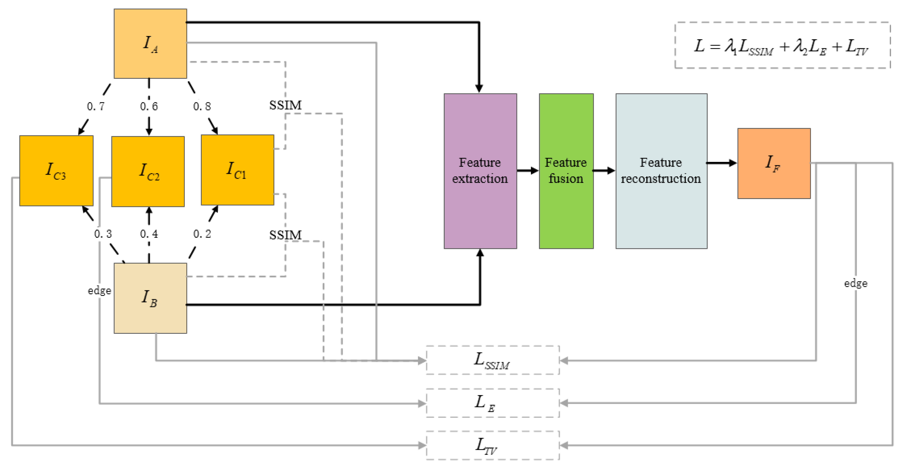
In this section, the construction of loss functions from SSIM, TV, and MSE will be discussed, and the fusion images IC obtained by adding visible and infrared images will be introduced to better describe the unsupervised fusion task. The overall structure of the loss function is shown in Figure 2.
The loss function consists of three components, LSSIM, LE, and LTV, where LSSIM is the main component and is used to compare the similarity of input and output, LE is the edge loss and is used to enhance the infrared edge information in the fused image, and LTV is the noise reduction loss and is used for image noise reduction. λ 1 and λ 2 are two parameters referred to in Reference [22]. LE and LTV are 103 times different from LSSIM in value. Therefore, the two parameters, λ 1 and λ 2 , are introduced. The total loss function L is shown in Equation (1):
L = λ 1 L S S I M + λ 2 L E + L T V
The SSIM loss LSSIM is obtained by Equation (2)
L S S I M = 1 1 N W = 1 N F S S I M ( W )
where the final fused image related to the infrared image and the visible image is represented by the FSSIM composed of SSIM. SSIM [27] denotes a method for measuring the structural similarity of two images, which compares the structural similarity of each component of the two images by a sliding window. The sliding window W moves from the top left to the bottom right in the image to determine the overall similarity between the two. The parameter N represents the total number of sliding windows in a single image. As suggested in [27], the window size is set to 11 × 11 in our study.
In FSSIM, the image IC1 is obtained by adding image IA and IB, which can be changed by adjusting the contribution of IA and IB. Image IC1 is treated as a kind of scale, and its similarity with images IA and IB is compared in the sliding window. The parts of images IA and IB with high similarity to IC1 are selected to form a loss with the final fused image IF. The FSSIM is shown in Equation (3).
F S S I M ( W ) = S S I M ( A , F | W )   , S S I M ( A , C 1 | W ) S S I M ( B , C 1 | W ) S S I M ( B , F | W ) , S S I M ( A , C 1 | W ) < S S I M ( B , C 1 | W )
When S S I M ( A , C 1 | W ) exceeds or is equal to S S I M ( B , C 1 | W ) , more information from image IA is presented in the sliding window of IC1, and SSIM directs the network to retain more information from image IA in the region of the fused image IF. By changing the proportion of images IA and IB in IC1, the retention degree of infrared and visible information in the fused image can be altered. IC1 is used as a scale in the loss to determine whether this region of the fused image for comparison contains more visible or infrared information. For example, when IC1 has a higher similarity to the visible image, the fused image is made to contain more visible information in this region. The overall tendency of the final fused image is then determined by adjusting IC1. According to the characteristics of the water surface image, in our study, image IC1 is obtained by adding 80% of visible image IA and 20% of infrared image IB.
LE is introduced to represent more texture details in the fused image, as shown in Equation (4), and denote the edge texture of images IF and IC2 extracted by the canny operator, where IC2 is obtained by summing 60% of image IA and 40% of image IB. Then, their mean square error (MSE) is calculated for the edge texture information of the two images.
L E = M S E ( e d g e F , e d g e C 2 )
To achieve gradient conversion and noise reduction, the total variation function is introduced as follows:
R ( i , j ) = I C 3 ( i , j ) I F ( i , j )
L T V = i , j ( | | R ( i , j + 1 ) R ( i , j ) | | 2 + | | R ( i + 1 , j ) R ( i , j ) | | 2 )
where R ( i , j ) denotes the difference between the image IC3 and the fused image IF, and | | | | 2 denotes the l2 distance. Since there are differences in the order of magnitude among the three loss functions, two hyperparameters λ 1 and λ 2 are set. Based on the outcomes of various experiments, λ 1 and λ 2 are set to 2000 and 10, respectively.

3.3. Training

A total of 2000 pairs of infrared and visible images were selected from the MIT Sea Grant Marine Autonomy Dataset Project. The dataset contains the viewpoint data of the ship in different locations and light conditions. The images were adjusted to 512 × 512 and used for training without any manual annotation. In addition, the network was trained for 200 epochs, and the loss was minimized using the Adam optimizer with a learning rate of 10−2. Our network was implemented on PyTorch [28] and trained on a PC with an Intel(R) Xeon(R) Gold 5320 2.20 GHz CPU, 32 GB RAM, and an NVIDIA RTX A4000 GPU.

4. Experimental Results and Analysis

In this section, some experiments and comparisons are presented to verify the effectiveness of F2F. Three pairs of infrared visible source photos from various situations are selected, as shown in Figure 3, and named as Example A, Example B, and Example C, respectively. These three pairs of photos serve as examples for later comparison and investigation.

4.1. Experimental Setting

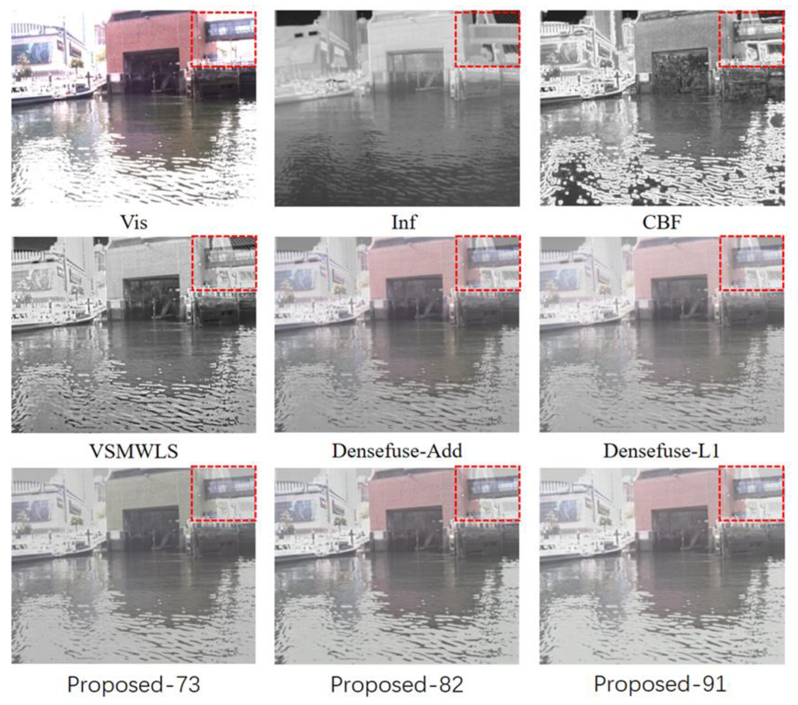
Several algorithms are selected for comparison in the experiments, including CBF [29], VSMWLS [30], Densefuse-Add [11], and Densefuse-L1 [11]. All four comparative methods were implemented based on publicly available codes, where the parameters were set according to the original papers. Several different IC1 images are compared to comprehend the impact of various IC1 images on the final fusion effect. For instance, Proposed-73 denotes that 70% of image IA and 30% of image IB are added to create IC1. Proposed-82 and Proposed-91 are defined in the same way as Proposed-73. The comparison results are shown in Figure 4, Figure 5 and Figure 6. Areas that need to be highlighted are marked by red dashed boxes.
The subjective visual assessment system is susceptible to human factors, such as eyesight, subjective preference, and individual emotion. Moreover, there is an insignificant difference among the fused results in most cases based on subjective evaluation. Thus, analyzing the fusion performance based on quantitative evaluation is indispensable. Seven quality metrics are utilized to quantitatively compare our fusion method with other existing algorithms: QAB/F [31] the sum of the correlations of differences (SCD) [32]; modified structural similarity for no-reference image (SSIMa) [11]; a new no-reference image fusion performance measure (MS-SSIM) [33]; and entropy (En) and nonlinear correlation information entropy (QNCIE) [34].
QAB/F measures the amount of edges transferred from the source images to the fused image. It is defined as follows:
Q A B / F = N i = 1 M j = 1 Q A F ( i , j ) w A ( i , j ) + Q B F ( i , j ) w B ( i , j ) N i M j w A ( i , j ) + w B ( i , j )
where Q A F ( i , j ) = Q g A F ( i , j ) Q o A F ( i , j ) , Q g A F ( i , j ) and Q o A F ( i , j ) are the edge strength and orientation preservation value at the location (i, j), respectively. N and M are the size of the image, and QBF(i, j) is similar to QAF(i, j), wA(i, j), and wB(i, j) denote the weights of QAF(i, j) and QBF(i, j), respectively.
The sum of the correlations of differences (SCD) is used to measure the information correlation between the fused image and the source image. The aim of the image fusion is to merge the images that depict the same scene with different sensing technology. The most meaningful fused image contains the maximum amount of complementary information transferred from the input images. It is formulated as follows:
SCD = r D 1 , S 1 + r D 2 , S 2
where r(.) function calculates correlation between S1 and D1, and S2 and D2 as:
r D k , S k = i j D k ( i , j ) D ¯ k S k ( i , j ) S ¯ k i j D k ( i , j ) D ¯ k 2 i j S k ( i , j ) S ¯ k 2
where k = 1, 2 and S ¯ k and D ¯ k are the average of the pixel values of Sk and Dk, respectively.
The SSIM [27] is an effective measure of structural similarity between two different images. It was first proposed by the University of Texas at Austin and the Laboratory of Image and Video Engineering, and combines the three components of luminance, structure, and contrast to comprehensively measure image quality. Let X be the reference image and Y be a test image, which is described as follows:
S S I M ( X , Y ) = 2 μ X μ Y + C 1 2 σ X Y + C 2 μ X 2 + μ Y 2 + C 1 σ X 2 + σ Y 2 + C 2
where μ and σ denote the mean and standard deviation, respectively, and σXY is the cross-correlation between X and Y. C1 and C2 are stable coefficients when the mean value and the variance are close to zero, which are two small constants. The standard deviation of the Gaussian window is set to 1.5 in the calculation.
The SSIMa is calculated by Equation (10):
S S I M a ( F ) = S S I M F , I 1 + S S I M F , I 2 × 0.5
where SSIM(·) denotes the structural similarity operation, F is the fused image, and I1, and I2 are source images. The value of SSIMa represents the ability to preserve structural information.
MS-SSIM is a multi-scale SSIM method for image quality assessment:
MS-SSIM ( x , y ) = l m ( x , y ) α M M j = 1 c j ( x , y ) β j s j ( x , y ) γ j
where c j ( x , y ) and s j ( x , y ) indicate contrast comparison and structure comparison, respectively, and 1 indicates brightness comparison. The exponents αM, βj and γj are used to adjust the relative importance of different components.
Information entropy (En) reflects the richness of information in an image. In general, the greater the amount of information in an image, the greater the information entropy, whose mathematical expression is as follows:
E n = L x = 0 p ( x ) log 2 p ( x )
QNCIE measures nonlinear correlation entropy between the source image and the fused image, and is defined as follows:
Q N C I E = 1 + 3 i = 1 λ i 3 log 256 λ i 3
where λi is the eigenvalue of the nonlinear correlation matrix.
For each of these metrics, the largest score indicates the best fusion performance.

4.2. Fusion Method Evaluation

The fused images obtained from multiple methods are shown in Figure 4, Figure 5 and Figure 6. Because CBF and VSMWLS only use grayscale maps for fusion, image color is not considered, and only texture information is compared.
As shown in the red box in Figure 4, the fused images obtained by CBF, VSMWLS, Densefuse-Add, and Densefuse-L1 do not naturally overlap objects such as trees. However, there is a natural excess of leaf edge in our algorithm.
The sky is frequently depicted as the background in images with water. Additionally, the typical fusion algorithms frequently result in color breaks in the sky, as shown in Figure 5, which does not occur in our algorithm. As can be seen from Figure 5, the ripples on the water surface are cleaner in our algorithm compared with other algorithms, reducing the interference in the image.
Figure 6 shows how different algorithms preserve some IR-specific information in the fused image. However, our algorithm can preserve as much infrared data as possible while keeping the brightness of the sky.
In our proposed fusion algorithm, Proposed-73, Proposed-82, and Proposed-91 have similar but different performance. Proposed-73 has some distortion in color performance as seen in Figure 4; Proposed-91 has some overexposure in bright areas; and Proposed-82 has the best performance in general.
In addition to the subjective evaluation, a few objective evaluation indicators were established. The average values of seven metrics for 18 fused images obtained by the existing methods and the proposed fusion method are shown in Table 1.
In Table 1, The best value in the objective indicator is shown in bold. It can be found that our algorithm has four optimal values in six metrics. The optimal values of QAB/F and SCD indicate that our algorithm is more natural and has lower noise, while the optimal values of MS-SSIM and QNCIE indicate that the structural information is well retained.
Our algorithm performs better in both subjective evaluation and objective metrics, which demonstrates that it is an effective IR-visible fusion algorithm for the surface water environment. Our algorithm still has some shortcomings. During the operation of the machine used in this paper, it took about 0.156 s to test one image. Therefore, our algorithm is still some distance away from completing real-time video tasks.

5. Conclusions

In this study, a novel and effective deep learning architecture based on CNN and dense block is proposed for the infrared and visible image fusion task. By combining the intermediate image IC created from two input images, it can more effectively describe the fusion task by balancing multiple inputs and a single output. The algorithm works well for water surface images.
The network consists of an encoder, a fusion layer, and a decoder, and the loss function consists of SSIM, TV, and MSE. The fused images IC1, IC2, and IC3 are introduced to better guide the network to complete the fusion task.
In addition, suitable parameters are set and compared with various methods, which achieved better results in some indicators. As a result, our algorithm produces better results and is specifically designed for the water surface scenario.
The goal of the infrared-visible fusion task is to combine the information from infrared and visible images while maintaining the color and texture information from each image separately. In addition to enhancing feature extraction capability, the challenge of this task is how to better describe the task objective. For future research, we aim to improve the real-time performance of the fusion algorithm and apply it to video fusion.

Author Contributions

Conceptualization, C.L.; methodology, C.L.; software, C.L.; validation, C.L.; formal analysis, C.L.; investigation, C.L.; resources, C.L.; data curation, C.L.; writing—original draft preparation, C.L.; writing—review and editing, Z.Z.; visualization, Z.Z.; supervision, Z.D. and H.Q.; project administration, H.Q.; funding acquisition, H.Q. and Z.Z. All authors have read and agreed to the published version of the manuscript.

Funding

This research was funded by the National Natural Science Foundation of China, grants 52025111 and 51939003, and in part by the Research Fund from Science and Technology on Underwater Vehicle Technology Laboratory, grant 2021JCJQ-SYSJJ-LB06911.

Institutional Review Board Statement

Not applicable.

Informed Consent Statement

Not applicable.

Data Availability Statement

Restrictions apply to the availability of these data. Data were obtained from MIT Sea Grant Marine Autonomy Dataset Project and are available from https://seagrant.mit.edu/auv-lab/ (accessed on 20 October 2022) with the permission of the MIT Sea Grant Marine Autonomy Dataset Project.

Conflicts of Interest

The authors declare no conflict of interest. The funders had no role in the design of the study; in the collection, analyses, or interpretation of data; in the writing of the manuscript; or in the decision to publish the results.

References

  1. Ben Hamza, A.; He, Y.; Krim, H.; Willsky, A. A multiscale approach to pixel-level image fusion. Integr. Comput. Eng. 2005, 12, 135–146. [Google Scholar] [CrossRef]
  2. Zhang, Q.; Fu, Y.; Li, H.; Zou, J. Dictionary learning method for joint sparse representation-based image fusion. Opt. Eng. 2013, 52, 057006. [Google Scholar] [CrossRef]
  3. Gao, R.; Vorobyov, S.A.; Zhao, H. Image Fusion with Cosparse Analysis Operator. IEEE Signal Process. Lett. 2017, 24, 943–947. [Google Scholar] [CrossRef]
  4. Zong, J.-J.; Qiu, T.-S. Medical image fusion based on sparse representation of classified image patches. Biomed. Signal Process. Control. 2017, 34, 195–205. [Google Scholar] [CrossRef]
  5. Li, H.; Wu, X.-J. Multi-focus Image Fusion Using Dictionary Learning and Low-Rank Representation. In Image and Graphics; Zhao, Y., Kong, X., Taubman, D., Eds.; Springer International Publishing: Cham, Switzerland, 2017; pp. 675–686. [Google Scholar] [CrossRef]
  6. Liu, Y.; Chen, X.; Peng, H.; Wang, Z. Multi-focus image fusion with a deep convolutional neural network. Inf. Fusion 2017, 36, 191–207. [Google Scholar] [CrossRef]
  7. Melekhov, I.; Kannala, J.; Rahtu, E. Siamese network features for image matching. In Proceedings of the 2016 23rd International Conference on Pattern Recognition (ICPR), Cancun, Mexico, 4–8 December 2016; pp. 378–383. [Google Scholar] [CrossRef]
  8. Wu, W.; Qiu, Z.; Zhao, M.; Huang, Q.; Lei, Y. Visible and infrared image fusion using NSST and deep Boltzmann machine. Optik 2018, 157, 334–342. [Google Scholar] [CrossRef]
  9. Li, H.; Wu, X.-J.; Kittler, J. Infrared and Visible Image Fusion using a Deep Learning Framework. In Proceedings of the 2018 24th International Conference on Pattern Recognition (ICPR), Beijing, China, 20–24 August 2018. [Google Scholar] [CrossRef]
  10. Deng, J.; Dong, W.; Socher, R.; Li, L.-J.; Li, K.; Fei-Fei, L. ImageNet: A large-scale hierarchical image database. In Proceedings of the 2009 IEEE Conference on Computer Vision and Pattern Recognition, Miami, FL, USA, 20–25 June 2009; pp. 248–255. [Google Scholar] [CrossRef]
  11. Li, H.; Wu, X.-J. DenseFuse: A Fusion Approach to Infrared and Visible Images. IEEE Trans. Image Process. 2019, 28, 2614–2623. [Google Scholar] [CrossRef]
  12. Pu, T. Contrast-based image fusion using the discrete wavelet transform. Opt. Eng. 2000, 39, 2075. [Google Scholar] [CrossRef]
  13. Burt, P.; Adelson, E. The Laplacian Pyramid as a Compact Image Code. IEEE Trans. Commun. 1983, 31, 532–540. [Google Scholar] [CrossRef]
  14. Do, M.; Vetterli, M. The contourlet transform: An efficient directional multiresolution image representation. IEEE Trans. Image Process. 2005, 14, 2091–2106. [Google Scholar] [CrossRef]
  15. Da Cunha, A.; Zhou, J.; Do, M. The Nonsubsampled Contourlet Transform: Theory, Design, and Applications. IEEE Trans. Image Process. 2006, 15, 3089–3101. [Google Scholar] [CrossRef]
  16. Luo, X.; Zhang, Z.; Zhang, B.; Wu, X. Image Fusion with Contextual Statistical Similarity and Nonsubsampled Shearlet Transform. IEEE Sensors J. 2016, 17, 1760–1771. [Google Scholar] [CrossRef]
  17. Yang, X.; Wang, J.; Zhu, R. Random Walks for Synthetic Aperture Radar Image Fusion in Framelet Domain. IEEE Trans. Image Process. 2017, 27, 851–865. [Google Scholar] [CrossRef]
  18. Quan, S.; Qian, W.; Guo, J.; Zhao, H. Visible and infrared image fusion based on Curvelet transform. In Proceedings of the The 2014 2nd International Conference on Systems and Informatics (ICSAI 2014), Shanghai, China, 15–17 November 2014; pp. 828–832. [Google Scholar] [CrossRef]
  19. Ahmed, N.; Natarajan, T.; Rao, K. Discrete Cosine Transform. IEEE Trans. Comput. 1974, C-23, 90–93. [Google Scholar] [CrossRef]
  20. Liu, Y.; Chen, X.; Ward, R.K.; Wang, Z.J. Image Fusion with Convolutional Sparse Representation. IEEE Signal Process. Lett. 2016, 23, 1882–1886. [Google Scholar] [CrossRef]
  21. Prabhakar, K.R.; Srikar, V.S.; Babu, R.V. DeepFuse: A Deep Unsupervised Approach for Exposure Fusion with Extreme Exposure Image Pairs. In Proceedings of the 2017 IEEE International Conference on Computer Vision (ICCV), Venice, Italy, 22–29 October 2017; pp. 4724–4732. [Google Scholar] [CrossRef]
  22. Hou, R.; Zhou, D.; Nie, R.; Liu, D.; Xiong, L.; Guo, Y.B.; Yu, C. VIF-Net: An Unsupervised Framework for Infrared and Visible Image Fusion. IEEE Trans. Comput. Imaging 2020, 6, 640–651. [Google Scholar] [CrossRef]
  23. Huang, G.; Liu, Z.; van der Maaten, L.; Weinberger, K.Q. Densely Connected Convolutional Networks. In Proceedings of the IEEE Conference on Computer Vision and Pattern Recognition (CVPR), Honolulu, HI, USA, 21–26 July 2017; pp. 2261–2269. [Google Scholar] [CrossRef]
  24. Woo, S.; Park, J.; Lee, J.Y.; Kweon, I.S. CBAM: Convolutional block attention module. In Computer Vision—ECCV 2018; Ferrari, V., Hebert, M., Sminchisescu, C., Weiss, Y., Eds.; Springer International Publishing: Cham, Switzerland, 2018; pp. 3–19. [Google Scholar] [CrossRef]
  25. Ioffe, S.; Szegedy, C. Batch normalization: Accelerating deep network training by reducing internal covariate shift. In Proceedings of the 32nd International Conference on International Conference on Machine Learning, Lille, France, 6–11 July 2015; JMLR.org: Lille, France, 2015; Volume 37, pp. 448–456. [Google Scholar]
  26. Glorot, X.; Bordes, A.; Bengio, Y. Deep Sparse Rectifier Neural Networks. In Proceedings of the Fourteenth International Con-ference on Artificial Intelligence and Statistics, JMLR Workshop and Conference Proceedings, Fort Lauderdale, FL, USA, 11–13 April 2011; pp. 315–323. [Google Scholar]
  27. Wang, Z.; Bovik, A.C.; Sheikh, H.R.; Simoncelli, E.P. Image Quality Assessment: From Error Visibility to Structural Similarity. IEEE Trans. Image Process. 2004, 13, 600–612. [Google Scholar] [CrossRef]
  28. Paszke, A.; Gross, S.; Massa, F.; Lerer, A.; Bradbury, J.; Chanan, G.; Killeen, T.; Lin, Z.; Gimelshein, N.; Antiga, L.; et al. PyTorch: An Imperative Style, High-Performance Deep Learning Library. Adv. Neural Inf. Process. Syst. 2019, 32. [Google Scholar]
  29. Kumar, B.K.S. Image fusion based on pixel significance using cross bilateral filter. Signal Image Video Process. 2013, 9, 1193–1204. [Google Scholar] [CrossRef]
  30. Ma, J.; Zhou, Z.; Wang, B.; Zong, H. Infrared and visible image fusion based on visual saliency map and weighted least square optimization. Infrared Phys. Technol. 2017, 82, 8–17. [Google Scholar] [CrossRef]
  31. Xydeas, C.; Petrović, V. Objective image fusion performance measure. Electron. Lett. 2000, 36, 308–309. [Google Scholar] [CrossRef]
  32. Aslantas, V.; Bendes, E. A new image quality metric for image fusion: The sum of the correlations of differences. AEU-Int. J. Electron. Commun. 2015, 69, 1890–1896. [Google Scholar] [CrossRef]
  33. Wang, Z.; Simoncelli, E.P.; Bovik, A.C. Multiscale structural similarity for image quality assessment. In Proceedings of the Thrity-Seventh Asilomar Conference on Signals, Systems & Computers, Pacific Grove, CA, USA, 9–12 November 2003. [Google Scholar] [CrossRef]
  34. Klonus, S.; Ehlers, M. Performance of evaluation methods in image fusion. In Proceedings of the 2009 12th International Conference on Information Fusion, Seattle, WA, USA, 6–9 July 2009; pp. 1409–1416. [Google Scholar]
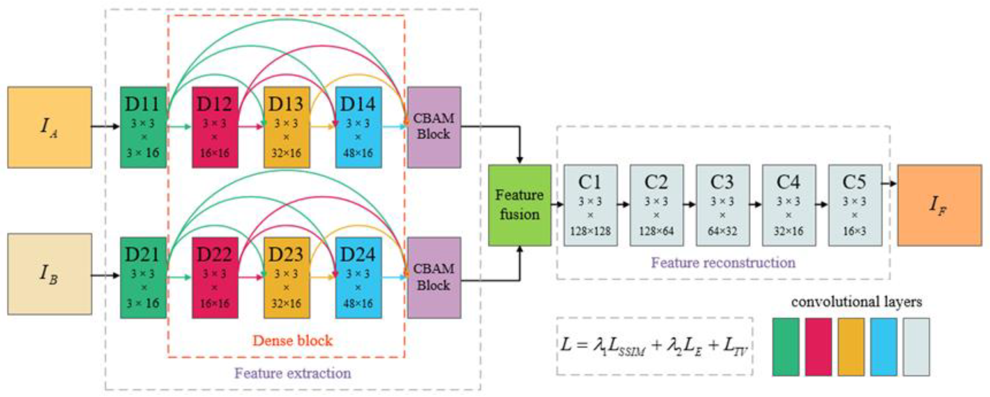
Figure 1. The architecture of the proposed F2F.
Jmse 11 00902 g001
Figure 2. The loss function of the proposed F2F.
Jmse 11 00902 g002
Figure 3. Three pairs of source images.
Jmse 11 00902 g003
Figure 4. The fusion results of different algorithms in Example A.
Jmse 11 00902 g004
Figure 5. The fusion results of different algorithms in Example B.
Jmse 11 00902 g005
Figure 6. The fusion results of different algorithms in Example C.
Jmse 11 00902 g006
Table 1. The average values of quality metrics.
MethodsQAB/FSCDSSIMMS-SSIMENQNCIE
CBF0.3613830.68900.5916280.7449727.6265910.810328431
VSMWLS0.3614811.45200.6839220.8319897.3669220.810889691
Densefuse-Add0.3737911.26580.7299810.8452926.9655330.811113586
Densefuse-L10.3710511.09670.7154350.8416396.8470640.811168666
Ours-910.3976231.28790.7128710.8556696.7902400.818237040
Ours-820.4003241.22670.7140100.8683776.8483200.817008603
Ours-730.3693661.20590.7159490.8465166.8277030.817501251
Disclaimer/Publisher’s Note: The statements, opinions and data contained in all publications are solely those of the individual author(s) and contributor(s) and not of MDPI and/or the editor(s). MDPI and/or the editor(s) disclaim responsibility for any injury to people or property resulting from any ideas, methods, instructions or products referred to in the content.