Article

Wind Speed Prediction Based on VMD-BLS and Error Compensation

1
School of Information and Control Engineering, Qingdao University of Technology, Qingdao 266520, China
2
State Key Laboratory of Industrial Control Technology, College of Control Science and Engineering, Zhejiang University, Hangzhou 310027, China
3
School of Automation, Central South University, Changsha 410012, China
4
College of Marine Electrical Engineering, Dalian Maritime University, Dalian 116026, China
*
Author to whom correspondence should be addressed.
J. Mar. Sci. Eng. 2023, 11(5), 1082; https://doi.org/10.3390/jmse11051082
Submission received: 20 April 2023 / Revised: 13 May 2023 / Accepted: 16 May 2023 / Published: 20 May 2023
(This article belongs to the Section Marine Energy)

Abstract

:
As one of the fastest-growing new energy sources, wind power technology has attracted widespread attention from all over the world. In order to improve the quality of wind power generation, wind speed prediction is an indispensable task. In this paper, an error correction-based Variational Mode Decomposition and Broad Learning System (VMD-BLS) hybrid model is proposed for wind speed prediction. First, the wind speed is decomposed into multiple components by the VMD algorithm, and then an ARMA model is established for each component to find the optimal number of sequence divisions. Second, the BLS model is used to predict each component, and the prediction results are summed to obtain the wind speed forecast value. However, in some traditional methods, there is always time lag, which will reduce the forecast accuracy. To deal with this, a novel error correction technique is developed by utilizing BLS. Through verification experiment with actual data, it proves that the proposed method can reduce the phenomenon of prediction lag, and can achieve higher prediction accuracy than traditional approaches, which shows our method’s effectiveness in practice.

1. Introduction

With the development of the times, traditional energy is no longer able to meet the rapidly growing energy consumption [1], and the fossil fuels are non-renewable resources, and their combustion can also bring serious environmental pollution [2]. Therefore, developing renewable and pollution-free energy is a hot issue in today’s society. In recent years, various new energy sources have been constantly emerging, among which wind power is one of the fastest growing renewable energy sources due to its advantages such as friendly to environment, zero carbon dioxide emissions, abundant resources, and cheap prices [3,4]. In 2021, renewable energy accounts for 38.3% of global electricity generation with wind power accounting for 6.7% [5]. In 2022, 78 GW wind capacity is installed globally, and this index can be expected to reach 115GW in 2023 [6].
However, although wind power has many advantages, it is a natural resource with intermittent, volatility, and unstable characteristics [7]. Therefore, it cannot generate sustained and stable electricity like traditional energy sources, such as thermal power. If the wind power is connected to the power grid directly without any optimization behaviors, it will introduce huge interference to the power system and leads to instability issues [8]. In particular, it may cause equipment damage or even large-scale power outages [9].
Wind speed prediction is one of the most effective methods to address the instability issues that arise with wind power generation [10]. By accurately forecasting wind speeds, wind farms can lower their operating costs, increase the competitiveness of wind power [11], and generate positive impacts [12]. Specifically, wind speed prediction can allow for reasonable adjustments to the power generation plan [13], optimize torque control to maximum utilization of wind power [14], and optimize layout of wind turbines, which will improve economic benefits for wind farms [15].
Early wind speed prediction methods generally use linear models, such as Autoregressive Moving Average (ARMA) [16], which assumes that future values are linearly correlated with historical data. However, linear models may not be sufficient to characterize the real world, because the real world is usually composed of linear and non-linear components [17]. After the 1990s, Artificial Intelligence (AI) gradually emerged, and various machine learning models have also emerged, such as Artificial Neural Networks (ANN) [18], Support Vector Machines (SVMs) [19], Extreme Learning Machines (ELMs) [20], etc. Many researchers have integrated these methods and proposed some hybrid wind prediction models [21,22]. However, wind speed is affected by many factors, such as temperature, air pressure, humidity, terrain, etc. If these data can not be collected because of some reasons, such as costs, we need to use historical data as the basis to predict wind speed. However, how much historical data to choose as the input is also worth considering. Too much data selection may cause a waste of machine performance and overfitting problem, while too little selection may lead to poor fitting results due to insufficient utilization of data information. This will lead to poor wind speed prediction results.
To improve the wind speed prediction accuracy, deep learning algorithms are introduced by researchers. In fact, it is widely used to deal with prediction problems. The Convolutional Neural Network (CNN) is employed to forecast ships’ electric consumption [23]. A Long Short-term Memory (LSTM) model is used to predict short-term wind power [24]. Recurrent Neural Network (RNN)-LSTM model is used to enhance the intra-day stock market prediction [25], and so on [26,27]. However, Deep Learning requires setting many parameters and long training time, which narrows its applications in practice. Moreover, most of the existing methods ignore the prediction lag which is brought by sharp changes in natural wind speed [26]. Obviously, this will increase the error between the actual wind speed and predicted values [3].
In order to select the appropriate data as input, reduce the occurrence of forecast lag, and improve the forecast accuracy of the univariate wind speed time series, this paper proposes a hybrid forecasting system of ARMA-VMD-BLS. First, the Variational Mode Decomposition (VMD) algorithm is used to decompose the original wind speed sequence into multiple components. Second, the ARMA model is used to select the appropriate amount of input data, and then the prediction results of each component used can be obtained by using the Broad Learning System (BLS) model. After obtaining the predicted results of each component, they are added up to obtain the wind speed prediction result. Moreover, in order to further improve the prediction accuracy, an error compensation method is proposed in this paper, which uses the BLS model to give the prediction error, and the final wind speed prediction result can be obtained by adding the error prediction result to the wind speed prediction result. Through the verification of real wind speed data, the proposed method can effectively alleviate the prediction lag phenomenon and improve the prediction accuracy. Compared with various machine learning models, the superiority of the BLS is proved.
The major contributions of this paper can be summarized as follows:
  • The VMD method is used to decompose data into multiple components and the ARMA model is used for each components to choose the optimal number of inputs. By this way, hidden features in the wind speed series can be extracted, and the forecast lags can be reduced.
  • The BLS model is utilized to predict each component, and the wind speed prediction result can be obtained by adding them. The BLS is a fast and efficient method, which is very suitable for wind speed forecasting.
  • An error compensation method is proposed to further improve the prediction accuracy. The BLS model is used to predict error, and the final wind speed prediction result is obtained by adding the error prediction result to the wind speed prediction result.
The rest of this article is organized as follows. Section 2 introduces the proposed method and mathematical models used. Section 3 is the experimental, which uses the real data validation of a wind farm in China to verify the feasibility of proposed method. Section 4 summarizes and draws conclusions.

2. The Proposed Method and Mathematical Models

2.1. The Framework of the Proposed Method

The flowchart is shown in Figure 1. In order to predict wind speed more accurately, this paper proposes a hybrid prediction model based on ARMA-VMD-BLS. As shown in Figure 1, the framework of proposed method includes the following content.
First, the VMD algorithm is used to decompose the original wind speed sequence into multiple Intrinsic Mode Functions (IMF). These IMF are extracted from the original data and have a fixed central frequency, which make them easy to be predicted. Second, the ARMA (p, q) model is built for each IMF to find the optimal number of inputs, and the p-values are used to partition each IMF. Third, the BLS is used to predict each IMF. Through the above steps, the wind speed prediction result can be obtained by adding up the prediction results of each IMF. Moreover, to deal with prediction lag phenomenon and further improve the forecast accuracy, a novel error compensation method is proposed in the paper. The error set is obtained by subtracting the predicted value from the real value. Then, the ARMA (p, q) model is built for the error set and the p-value is used to partition the error set. Finally, the BLS is used to predict the error, and the final wind speed prediction result can be obtained by adding the wind speed prediction result to the error prediction result.

2.2. The Detail Steps of the Proposed Method

Step 1: Use VMD to decompose the original wind speed sequence.
In this step, the VMD algorithm is used to decompose the original wind speed time series [28], which can extract potential patterns and remove noise from the original data, and obtain multiple components with fixed center frequencies. By this means, more wind speed features will be obtained, which is beneficial for improving prediction accuracy [7].
The VMD algorithm was proposed by Konstantin Dragomiretskiy and Dominique Zosso in 2014 [29]. Because it can effectively overcome problems, such as the dependence of Empirical Mode Decomposition (EMD) on extreme point selection and frequency overlap, the VMD has attracted increasing attention from researchers [30].
The VMD can decompose the wind speed time series into several IMF. Its expression is
u k ( t ) = A k ( t ) cos Φ k ( t ) ,
where A k ( t ) is the non-negative envelope, Φ k ( t ) is the phase and Φ k ( t ) 0 , u k ( t ) is the raw wind speed data decomposed to the k-th IMF.
The corresponding constrained variational model is as
min u k ω k K t δ ( t ) + j π t u k ( t ) e j ω k t 2 2 s . t . k u k ( t ) = f ,
where u k = u 1 , , u k is the set of all modes, ω k = ω 1 , , ω k is the set of center frequencies of all modes and f is the raw wind speed data.
To solve the constrained optimization problem Equation (2), the augmented Lagrangian function is used to convert the above equation constraint problem to an unconstrained problem
L u k , ω k , λ = α K t δ ( t ) + j π t u k ( t ) e j ω k t 2 2 + f ( t ) k u k ( t ) 2 2 + λ ( t ) , f ( t ) k u k ( t ) ,
where α is the penalty parameter, ∗ represents convolution operation, and λ is the Lagrangian multiplier.
Then, the Alternate Direction Method of Multipliers (ADMM) is used to update u k , ω k , and λ
u ^ k n + 1 ( ω ) = f ^ ( ω ) i k u ^ i ( ω ) + λ ^ ( ω ) 2 1 + 2 α ω ω k 2
ω k n + 1 = 0 ω u ^ k ( ω ) 2 d ω 0 u ^ k ( ω ) 2 d ω
λ ^ n + 1 ( ω ) = λ ^ n ( ω ) + τ f ^ ( ω ) k = 1 K u ^ k n + 1 ( ω ) .
Step 2: Use the ARMA model to select the optimal number of inputs.
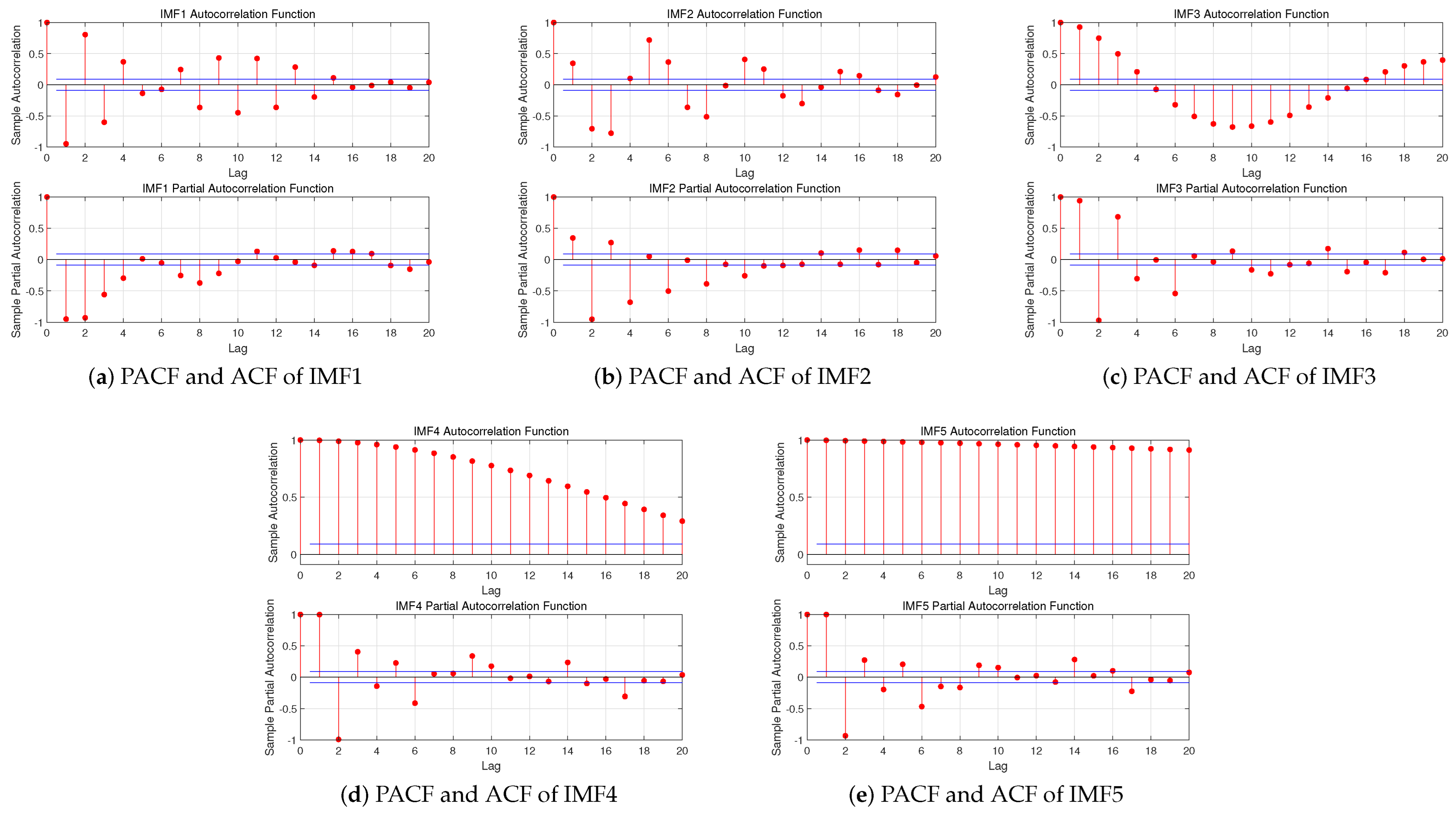
In the Step 2, we use training sets to establish ARMA model to find the optimal number of inputs. The training sets are the multiple IMF decomposed through VMD in Step 1, and then an ARMA (p, q) model is established for each IMF. Since the fact that the decomposed data belongs to a relatively stable sequence, there is no need for stationarity test and an ARMA model can be directly established. For each p and q in ARMA (p, q), we set a loop and use the Akaike Information Criterion (AIC) to find the optimal combination of (p, q). The resulting p-value is the optimal number of inputs we are looking for. It is worth noting that the optimal p-value corresponding to each IMF may be different. Thus, in the final summation, the same length needs to be selected for addition, which will be explained in detail later.
The ARMA (p, q) model is one of the earliest models used for time series prediction [31]. It consists of two models, the Autoregressive (AR) model and Moving Average (MA) model. The mathematical model is
X t = i = 1 p α i X t i + j = 1 q β j ϵ t j + ϵ t
where X = X 1 , X 2 , , X t is wind speed time series, X t is the current wind speed, α i and β j are the autoregressive and moving average parameter, p and q are important parameter called Partial Autocorrelation Coefficient (PAC) and Autocorrelation Coefficient (AC) and ϵ t is white nose of time t.
The ARMA model describes the relationship between current value, historical error, and historical value. From Equation (7), one can see that the current value X t is composed of a linear combination of p historical values and q historical errors. It also means that if every p datum is taken as a group, the internal correlation of this group is very strong. Thus, it is very reasonable to select p as the basis for dividing the univariate series.
Step 3: Use the p-value to partition data sequence.
In Step 2, the optimal p-values of each IMF was obtained. In this step, we will use them to partition data for each IMF. The specific method is that, for each IMF, starting from the first data, every p datum is a group, the first p−1 data are used as input, and the pth data are output. That is, the first p−1 data are used to predict the pth value. Then, starting from the second set of data, the previous steps are repeated until all the data are divided. This process can be described as Equation (8)
x p = f x 1 , x 2 , , x p 1 x p + 1 = f x 2 , x 3 , , x p x end = f x end p + 1 , x end p , , x end 1 ,
where x t represents the wind speed value at time t and f ( · ) represents the relationship between historical and current value.
Step 4: Use the BLS model to predict each IMF.
In this step, the divided data in Step 3 are used to train the BLS model. For each IMF, triple nested loops are used to find the optimal number of mapping nodes, windows in mapping feature layers, and enhancement nodes. The first 75% of the dataset is used as the training set, and the rest is used as the testing set. The result will be shown in the following section.
Compared with the deep learning system, BLS has a faster training process, and can increase the number of feature nodes and enhancement nodes through incremental learning. Therefore, the system can continuously update parameters without retraining, which is an alternative to deep learning [32].
The basic structure of BLS model is shown in Figure 2. It is based on the Random Vector Functional Link Neural Network (RVFLNN), which maps the input to the mapping layer through multiple sets of mappings. The mapping is ϕ X W e i + β e i in Figure 2, where X is the wind speed IMF decomposed by the VMD algorithm. W e i and β e i are respectively the random weights and bias with the proper dimensions. Each mapping corresponds to a mapping feature: Z 1 , Z 2 , , Z n . The nodes in the mapping feature are called mapping nodes. Each mapping feature is passed to the output layer and the enhancement layer, respectively. In the process of passing from the mapping layer to the enhancement layer, there will also be a layer of mapping, which is ξ X W e j + β e j in Figure 2, where W e j and β e j are the random weights and bias with the proper dimensions, respectively. The nodes in the enhancement layer are called enhancement nodes: H 1 , H 2 , , H n . Enhancement nodes and mapping nodes are finally connected to the output layer.
If one wants to train a model and the input X and labels Y are known, one can figure out w in Figure 2 by the equation
Y = A w ,
where A is the augmented matrix of the mapping layer matrix and enhancement layer matrix, that is, A = [ Z | H ] . Z and H can be figured out by X . Then, the w can be calculated as
w = A + Y ,
where A + is the pseudo-inverse matrix of A .
From Equations (9) and (10) we know that, the BLS inputs all the data into the system for training. There is no weight update process, and the weights are directly calculated, while deep learning needs to pass the data into the neural network one by one to update the weights continuously. Therefore, the training speed of BLS is significantly faster than that of deep learning.
In order to solve the problem that the model training cannot achieve the required accuracy, the author also proposed the BLS with incremental learning, including increasing the number of mapping nodes and enhancing nodes, and increasing the input data. In this paper, the incremental learning is used to find the best number of mapping nodes and enhancing nodes, which can improve the prediction accuracy.
Step 5: Add up prediction results of each IMF.
The predictions for each IMF using BLS model in Step 4 are not the true wind speed, we need to add all the predictions to obtain the wind speed prediction
R w s = R I M F 1 + R I M F 2 + + R I M F n ,
where R w s is the wind speed prediction result, and R I M F is the prediction result of each IMF.
Step 6: Get the prediction error of wind speed.
The error time series can also be predicted due to its non-linear characteristics [33]. If the predicted error can be added to the predicted wind speed, a more accurate prediction result can be obtained. In Step 4, the training model is obtained. In Step 5, we obtain the prediction result of the testing set. Furthermore, in this step, we subtract the predicted value from the real value of the testing set to obtain the error testing set. Specially, to construct the error training set, the training set is used as the input of the BLS model trained in Step 4 to obtain the prediction result of the training set, and then the error training set can be obtained by subtracting the predicted value from the real value of the training set
E t r = R t r r v R t r p v E t e = R t e r v R t e p v ,
where E t r and E t e represent error training set and error testing set, R t r r v and R t e r v represent the real value of training and testing set, and R t r p v and R t e p v are the prediction value of training and testing set, respectively.
Step 7: Build the ARMA model for error set and partition error set.
This step is very similar to Step 2 and Step 3. The error set obtained in Step 6 is also a univariate time series. Since its fluctuation is very small, there is no need to perform VMD like the original data. The ARMA model is used to select the optimal number of inputs p for the error set, and its p-value is used to divide the error training set and testing set. The way of division is the same as in Step 3, and only the value of p may be different
e p = g e 1 , e 2 , , e p 1 e p + 1 = g e 2 , e 3 , , e p e end = g e end p + 1 , e end p , , e end 1 ,
where x t represents the error value at time t and g ( · ) represents the relationship between historical and current error.
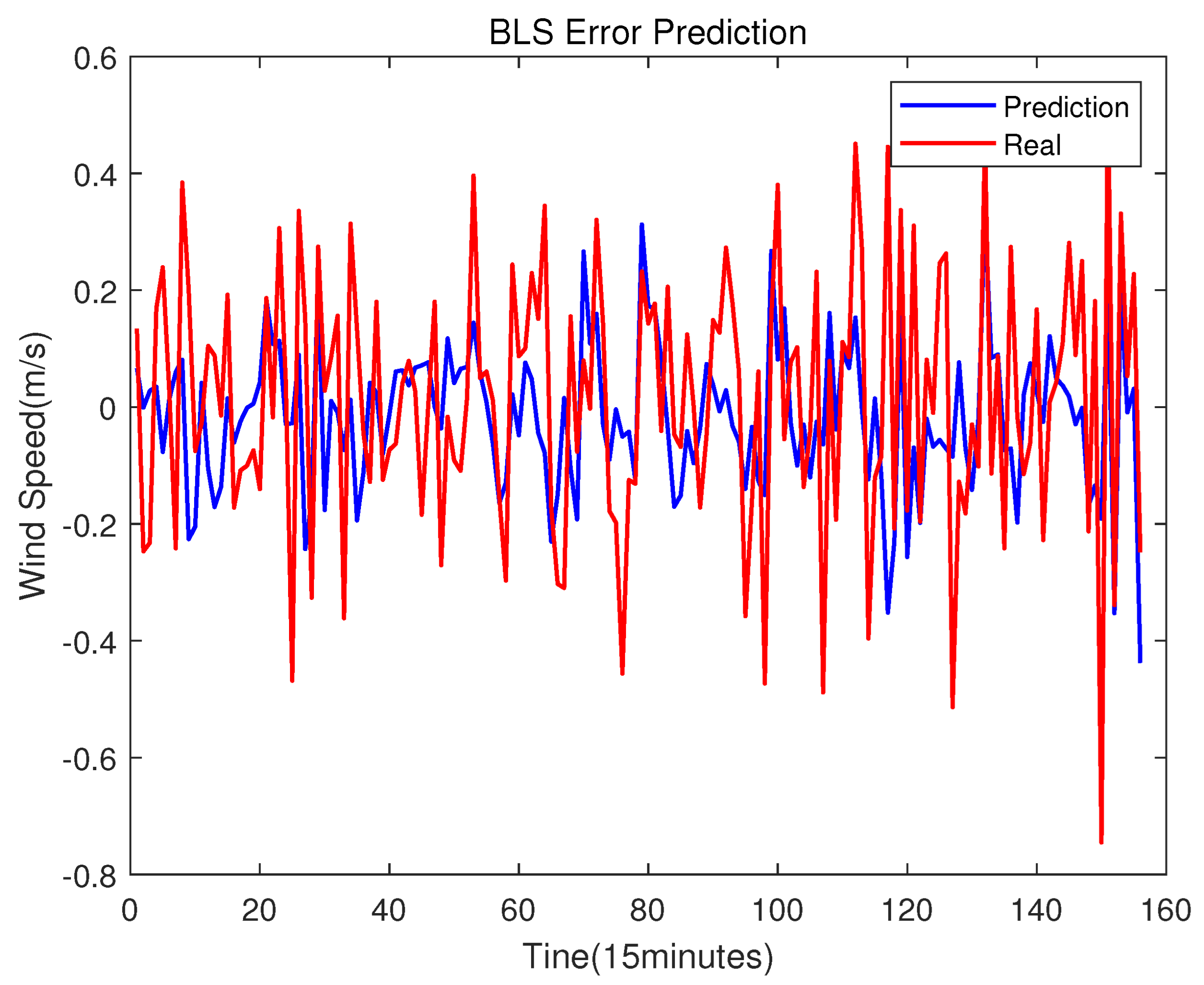
Step 8: Use the BLS model to predict error.
In this step, divided data in Step 7 are used to retrain the BLS model. For error training set, triple nested loops are used to find the optimal number of mapping nodes, windows in mapping feature layers and enhancement nodes. After that, the error testing set is used to check the prediction effect of the model. The result will be shown in the following section.
Step 9: Add the wind speed prediction result to the error prediction result.
This is the final step. The final wind speed prediction result will be obtained by adding the wind speed prediction result to the error prediction result
R f w s = R w s + R e r r ,
where R f w s is the final wind speed prediction result, and R e r r is the prediction result of error.

3. Experiment

This section mainly introduces the process and results of the experiment. Section 3.1 shows the wind speed prediction and Section 3.2 shows the error prediction. Furthermore, in order to prove the superiority of this method, Section 3.3 uses direct prediction and selects three models (SVE, BPNN and ELM) to replace the BLS model for comparison.
The raw wind speed data from a wind farm in China are shown in Figure 3. Among them, the data are recorded every 15 min, a total of 671 data are selected, the first 500 data are used as the training set, and the last 171 data are used as the testing set. The experiment is tested on a PC with AMD Ryzen 5800 H, NVDIA RTX 3070 Laptop and 16 GB memory. The name of our PC is Legion R9000P 2021, which is produced by Lenovo company, located in Beijing, China. The following is the experiment result.

3.1. Wind Speed Prediction

3.1.1. Use VMD to Decompose the Raw Data

It can be seen from Figure 3 that the fluctuation of this sequence is very large. If direct prediction is carried out, the problem of prediction lag may occur, which seriously affects the prediction accuracy. Therefore, five IMF are obtained by using the VMD algorithm to decompose the original data, and the results are shwon in Figure 4.
Here, the obtained IMF can be added and compared with the original data, as shown in Figure 5. It can be seen that the result of the decomposition fits well with the original data, which proves that the decomposition effect is good.

3.1.2. ARMA Modeling and Partitioning Data

For each IMF, an ARMA (p, q) model needs to be established separately to find its corresponding optimal p-value. Among them, p sets the cycle from 5 to 10, and q sets the cycle from 1 to 15. The p-value determines the number of historical data inputs. Using p-value to select the number of wind speed data inputs can solve some problems resulting from wrong input numbers, such as underfitting caused by too little data selection and overfitting problem caused by too much selection. The q-value is also an important parameter of the ARMA model. Therefore, it also needs to be selected carefully based on AIC. It is worth noting that finding the optimal p and q requires using the training set, not the entire dataset, since the testing set is considered unknown.
The values of p and q are related to the Autocorrelation Functions (ACF) and Partial Autocorrelation Functions (PACF) of each IMF, which are shown in Figure 6. Furthermore, the AIC criterion is used to find the optimal value. [34].
The optimal (p, q) of each IMF obtained by using the AIC criterion is shown in Table 1.
From Table 1, the optimal p of each IMF are obtained according to its minimum AIC value, and they are used to obtain data training and testing sets, as that of Step 3. By this means, the inputs for the BLS model can be found.

3.1.3. Train the BLS Model to Predict Wind Speed

For each IMF, it is necessary to establish a BLS model for prediction. In this step, a triple nested loops are set up to find the optimal number of mapping nodes, windows in mapping feature layers and enhancement nodes for each model. The results are shown in Table 2 below.
The trained optimal BLS model is used to predict each IMF, and the prediction results are shown in the following figures. From Figure 7 and Figure 8, it can be seen that for each IMF, the BLS model can predict well. Next, each prediction result is added and the wind speed prediction result can be obtained, which is shown in Figure 9.
From Figure 9, we can draw a conclusion that, after decomposing the original sequence by using the VMD method, the BLS model performs well in predicting wind speed.

3.2. Error Compensation

In order to compensate for the time lag and achieve a better prediction effect, this paper proposes an error correction method. The BLS model is trained by the historical error to predict future errors. Then, a more accurate wind speed prediction result can be obtained by adding the error prediction result to the wind speed prediction result.

3.2.1. Obtain Error Set

The error is the difference between the predicted value and the true value. According to Figure 7 and Figure 8, we can obtain the error training set and error testing set, which is shown in Figure 10.
Note that the error set in this paper is obtained by subtracting the predicted values from the real values, which is shown in Equation (12). By this means, the final wind speed prediction result can be obtained by adding the predicted error to the predicted wind speed. However, if one subtracts the real value from the predicted value to obtain the error set, the final wind speed prediction should be obtained by subtracting the predicted error from the predicted wind speed.

3.2.2. ARMA Modeling and Partitioning Error Data

The fluctuation of the error set is small, so there is no need to use VMD method, and the prediction can be made directly. However, the error set is still a univariate sequence. Therefore, it is also necessary to select the optimal p and q values through the ARMA model to divide the data to train model.
The ARMA model is built by using the error training set, since the testing set is considered unknown. The ACF and PACF of the error set is shown in Figure 11 and the optimal p and q results are shown in Table 3.
After dividing the data with the optimal p value, the dataset can be sent to the BLS model for training. The same training method as that of the raw data are used for error data of BLS: Triple nested loops are set to find the optimal number of mapping nodes, windows in mapping feature layers and enhancement nodes. The result is shown in the Table 4.
The error prediction results are shown in Figure 12. It can be seen from the figure that the prediction effect of BLS on the error is not as good as the prediction effect on IMF. This is because the regularity of the error sequence is not strong as the sequence after VMD precessing [26]. However, the prediction result does not need to be very accurate. The final wind speed prediction accuracy will also improve as long as the prediction value can reflect the change trend of the error.
Next, we add the error prediction result to the error prediction result, and the final wind speed prediction result is shown in Figure 13 below. It is worth noting that in the process of dividing the data, the number of datasets will inevitably decrease by p. This is because, in the process of using the first p-1 data to predict the p-th data, the first p-1 data cannot be predicted. However, it has no effect on the prediction accuracy, since we always want to predict the later data, and do not need the missing data in the front.
Here, the BLS prediction without error compensation result of the same time period (the first p-1 data points in the very beginning of the testing set are deleted to make the time period be the same as that of the error compensantion based method) is also shown as Figure 14 below.
This paper uses Root Mean Square Error (RMSE), Mean Absolute Percentage Error (MAPE) and Coefficient of Determination ( R 2 ) to evaluate the prediction effect of the model
R M S E = 1 N i = 1 N x ^ i x i 2
M A P E = 1 n t = 1 n x ^ i x i x ^ i
R 2 = 1 i = 1 N ( x i x i ^ ) 2 i = 1 N ( x i x ¯ ) 2 ,
where N is the number of samples, x i represents the ith value of the wind speed series, x ^ i represents the ith estimate value of the series and x ¯ is average value of samples, respectively.
In Figure 13 and Figure 14, the RMSE of BLS error compensation prediction result is 0.20634, while the RMSE of BLS prediction without error compensation is 0.22165. The result shows that after error compensation, the accuracy of prediction has increased by 6.9 % . Figure 15 shows that the prediction accuracy of the BLS with error compensation method is better than that of the BLS without error compensation. From Figure 13, Figure 14 and Figure 15, one can conclude that the prediction results after error compensation have been significantly improved.

3.3. Comparison

In order to prove the superiority of the VMD-BLS hybrid wind speed forecasting system proposed in this paper, this subsection uses the BLS model to directly predict the wind speed without the VMD method. Furthermore, three models of SVR, ELM, and BPNN are used to replace the BLS to carry out the error compensation.

3.3.1. BLS Direct Prediction

The direct prediction mentioned above means that the VMD method and error compensation are not used. The prediction results are shown in Figure 16.
In Figure 16, the prediction effect seems to be very good. However, if the figure is zoomed in, we will find that the predicted value always lags behind the real value, which will seriously affect the prediction accuracy. That is why the RMSE of testing set in Figure 16 is 0.6515, which is larger than that of the Figure 13 and Figure 14.
The reason of the time lag phenomenon is mainly caused by the non-stationary nature of the raw sequence [26]. Moreover, the time of predicted wind speed should be corresponding to the time of the real wind speed. Thus, although the time lag looks like a constant from the comparison figures between real wind speeds and predict ones, it is not appropriate to move the time step of predicted wind speed simply to eliminate the lag. Therefore, it is necessary to use VMD to process sequences to reduce the lag [35].

3.3.2. Different Models for Prediction

The SVR, BPNN, and ELM are used to replace the BLS model in the VMD-BLS hybrid system to predict each IMF. All the parameters of three models are selected by trial and error, which are shown in Table 5, Table 6 and Table 7. And the prediction results are in Figure 17.
From Figure 17, a conclusion can be drawn that all the three models can achieve a good result after the VMD method. Compared with the BLS direct prediction shown in Figure 16, the three models’ prediction results reduce the time lag and improve the accuracy.
However, compared with the BLS prediction with VMD method shown in Figure 9, the prediction effect of the three methods are still slightly worse than that of the BLS according to RMSE. The result proves that the BLS model is more suitable for wind speed prediction.
The evaluation indicators of the four models on the testing set are shown in Table 8. It can be seen that BLS model performs well on most indicators, only MAPE is slightly higher than the ELM model.

3.3.3. Different Models for Error Compensation

We have shown above that using the BLS model to predict the wind speed after VMD method is the best. Then, we will use different models to predict the error, and the prediction results will be added to the wind speed prediction results. The wind speed prediction results after different models error compensations are as follows.
It can be seen from Figure 18 that after error compensation, the prediction accuracy of the three models has been improved. Specifically, the accuracy of the ELM, SVR and BPNN has been improved by 6.0 % , 6.0 % and 7.2 % , respectively. However, the accuracy of these three models still has some gaps compared with BLS in Figure 13. Table 9 is the performance indicators of each model after error compensation.
From Table 9, the RMSE of the BLS model is the smallest and the R 2 is the biggest, which shows that the BLS model for error compensation is better than the other three models. The ELM model also performs well, and its performance indicators are better than that of the SVR and BPNN model. The SVR model has a good ability of describing non-linear relationship [22]. Thus, the performance of SVR is better than that of BPNN model. The performance of BPNN is worse than the other three models. More network layers and neuron nodes can be added in the BPNN, but it may cost more performance and waste more time to train. Therefore, the BLS model is more suitable for wind speed prediction.
Section 3.3 proves two things: one is that using VMD method to process the raw data can reduce the prediction lag phenomenon, and the other thing is that the error compensation technique can further improve the accuracy and the BLS model achieve the best accuracy in the four models.
Note that the accuracy increase is very large after using the VMD method to process the data to reduce the time lag, while the increase in error compensation may be small. However, the power generation base of wind farms is very large. Therefore, every 1 % increase in prediction accuracy will increase the power generation efficiency very significantly. Moreover, the cost of error compensation is very low because there is no need to capture additional data, and only the historical values of the predicted values need to be utilized. Thus, it makes sense for developing error compensation technique.

4. Conclusions

In this paper, a hybrid wind speed forecasting system based on VMD-BLS with error compensation is proposed, which is suitable for predicting univariate wind speed series. First, the wind speed sequence is decomposed into multiple IMF by the VMD algorithm. Second, an ARMA model is established for each IMF to find the optimal number of inputs. Then, the BLS model is used to predict the wind speed. In order to further improve the prediction accuracy, an error compensation method by using BLS model is proposed. The error is predicted by the BLS model, and the final wind speed prediction can be obtained by adding the error prediction result to the wind speed prediction result. After verification experiments with real data, it is proved that using VMD method to process the raw data can reduce the phenomenon of prediction lag and improve the accuracy of prediction result. Through the comparison BLS, ELM, SVR, and BPNN model, it shows the prediction effect of BLS is better than the other three models.
Although we have proposed some methods to improve forecast accuracy, there is still much room for improvement in this work. For example, a better prediction result can be obtained if a more accurate algorithm can be found to decompose the original data. Furthermore, it is also worth considering to make this method an online prediction system, which can continuously update the data. The online system is more in line with practical applications, and it is a very interesting research direction.

Author Contributions

Conceptualization, X.J.; Methodology, X.J.; Software, X.J. and D.Z.; Validation, D.Z. and H.W.; Formal analysis, D.M.; Resources, X.J. and D.M.; Writing—original draft, D.Z.; Writing—review & editing, X.J. and D.S.; Visualization, D.Z. and H.W.; Supervision, X.J., D.S. and Y.T.; Funding acquisition, X.J. and Y.T.. All authors have read and agreed to the published version of the manuscript.

Funding

This work was supported in part by the Shandong Provincial Nature Science Foundation of China under Grant ZR2021QF115, in part by the National Natural Science Foundation of China under Grant 62203249, and in part by the Lixian Scholar Project of Qingdao University of Technology.

Institutional Review Board Statement

Not applicable.

Informed Consent Statement

Not applicable.

Data Availability Statement

The data is unavailable due to privacy security.

Conflicts of Interest

The authors declare no conflict of interest.

Abbreviations

The following abbreviations are used in this manuscript:
ARMAAutoregressive Moving Average
BLSBroad Learning System
BPNNBackpropagation Neural Network
ELMExtreme Learning Machine
IMFIntrinsic Mode Functions
SVRSupport Vector Regression
VMDVariational Mode Decomposition

References

  1. Zhang, Y.; Zhao, Y.; Kong, C.; Chen, B. A new prediction method based on VMD-PRBF-ARMA-E model considering wind speed characteristic. Energy Convers. Manag. 2020, 203, 112254. [Google Scholar] [CrossRef]
  2. Song, D.; Yan, J.; Zeng, H.; Deng, X.; Yang, J.; Qu, X.; Rizk-Allah, R.M.; Snášel, V.; Joo, Y.H. Topological Optimization of an Offshore-Wind-Farm Power Collection System Based on a Hybrid Optimization Methodology. J. Mar. Sci. Eng. 2023, 11, 279. [Google Scholar] [CrossRef]
  3. Xu, X.; Hu, S.; Shi, P.; Shao, H.; Li, R.; Li, Z. Natural phase space reconstruction-based broad learning system for short-term wind speed prediction: Case studies of an offshore wind farm. Energy 2023, 262, 125342. [Google Scholar] [CrossRef]
  4. Sacie, M.; Santos, M.; López, R.; Pandit, R. Use of state-of-art machine learning technologies for forecasting offshore wind speed, wave and misalignment to improve wind turbine performance. J. Mar. Sci. Eng. 2022, 10, 938. [Google Scholar] [CrossRef]
  5. Fan, Q.; Wang, X.; Yuan, J.; Liu, X.; Hu, H.; Lin, P. A Review of the Development of Key Technologies for Offshore Wind Power in China. J. Mar. Sci. Eng. 2022, 10, 929. [Google Scholar] [CrossRef]
  6. GWEC Global Wind Report. 2023. Available online: https://gwec.net/globalwindreport2023/ (accessed on 19 April 2023).
  7. Xu, W.; Liu, P.; Cheng, L.; Zhou, Y.; Xia, Q.; Gong, Y.; Liu, Y. Multi-step wind speed prediction by combining a WRF simulation and an error correction strategy. Renew. Energy 2021, 163, 772–782. [Google Scholar] [CrossRef]
  8. Sun, G.; Jiang, C.; Cheng, P.; Liu, Y.; Wang, X.; Fu, Y.; He, Y. Short-term wind power forecasts by a synthetical similar time series data mining method. Renew. Energy 2018, 115, 575–584. [Google Scholar] [CrossRef]
  9. Du, Y.; Zhou, S.; Jing, X.; Peng, Y.; Wu, H.; Kwok, N. Damage detection techniques for wind turbine blades: A review. Mech. Syst. Signal Process. 2020, 141, 106445. [Google Scholar] [CrossRef]
  10. Wang, X.; Guo, P.; Huang, X. A review of wind power forecasting models. Energy Procedia 2011, 12, 770–778. [Google Scholar] [CrossRef]
  11. Jung, J.; Broadwater, R.P. Current status and future advances for wind speed and power forecasting. Renew. Sustain. Energy Rev. 2014, 31, 762–777. [Google Scholar] [CrossRef]
  12. Song, D.; Li, Z.; Deng, X.; Dong, M.; Huang, L.; Yang, J.; Su, M.; Joo, Y. Deep optimization of model predictive control performance for wind turbine yaw system based on intelligent fuzzy deduction. Expert Syst. Appl. 2023, 221, 119705. [Google Scholar] [CrossRef]
  13. Zhang, Y.; Yang, J.; Wang, K.; Wang, Z. Wind power prediction considering nonlinear atmospheric disturbances. Energies 2015, 8, 475–489. [Google Scholar] [CrossRef]
  14. Jiao, X.; Zhou, X.; Yang, Q.; Zhang, Z.; Liu, W.; Zhao, J. An improved optimal torque control based on estimated wind speed for wind turbines. In Proceedings of the 2022 13th Asian Control Conference (ASCC), Jeju, Republic of Korea, 4–7 May 2022; pp. 2024–2029. [Google Scholar]
  15. Tang, X.; Yang, Q.; Wang, K.; Stoevesandt, B.; Sun, Y. Optimisation of wind farm layout in complex terrain via mixed-installation of different types of turbines. IET Renew. Power Gener. 2018, 12, 1065–1073. [Google Scholar] [CrossRef]
  16. Hannan, E.J. The estimation of the order of an ARMA process. Ann. Stat. 1980, 8, 1071–1081. [Google Scholar] [CrossRef]
  17. de Oliveira, J.F.; Silva, E.G.; de Mattos Neto, P.S. A hybrid system based on dynamic selection for time series forecasting. IEEE Trans. Neural Networks Learn. Syst. 2021, 33, 3251–3263. [Google Scholar] [CrossRef] [PubMed]
  18. Ordulj, M.; Šantić, D.; Matić, F.; Jozić, S.; Šestanović, S.; Šolić, M.; Veža, J.; Ninčević Gladan, Ž. Analysis of the Influence of Seasonal Water Column Dynamics on the Relationship between Marine Viruses and Microbial Food Web Components Using an Artificial Neural Network. J. Mar. Sci. Eng. 2023, 11, 639. [Google Scholar] [CrossRef]
  19. Alshahri, A.H.; Elbisy, M.S. Assessment of Using Artificial Neural Network and Support Vector Machine Techniques for Predicting Wave-Overtopping Discharges at Coastal Structures. J. Mar. Sci. Eng. 2023, 11, 539. [Google Scholar] [CrossRef]
  20. Zhang, C.; Ding, M.; Wang, W.; Bi, R.; Miao, L.; Yu, H.; Liu, L. An improved ELM model based on CEEMD-LZC and manifold learning for short-term wind power prediction. IEEE Access 2019, 7, 121472–121481. [Google Scholar] [CrossRef]
  21. Liu, M.; Cao, Z.; Zhang, J.; Wang, L.; Huang, C.; Luo, X. Short-term wind speed forecasting based on the Jaya-SVM model. Int. J. Electr. Power Energy Syst. 2020, 121, 106056. [Google Scholar] [CrossRef]
  22. Jiao, X.; Yang, Q.; Xu, B. Hybrid intelligent feedforward-feedback pitch control for VSWT with predicted wind speed. IEEE Trans. Energy Convers. 2021, 36, 2770–2781. [Google Scholar] [CrossRef]
  23. Kim, J.Y.; Oh, J.S. Electric Consumption Forecast for Ships Using Multivariate Bayesian Optimization-SE-CNN-LSTM. J. Mar. Sci. Eng. 2023, 11, 292. [Google Scholar] [CrossRef]
  24. Shahid, F.; Zameer, A.; Muneeb, M. A novel genetic LSTM model for wind power forecast. Energy 2021, 223, 120069. [Google Scholar] [CrossRef]
  25. Kumar, K.; Haider, M.T.U. Enhanced prediction of intra-day stock market using metaheuristic optimization on RNN–LSTM network. New Gener. Comput. 2021, 39, 231–272. [Google Scholar] [CrossRef]
  26. Zhang, Z.; Li, M.; Lin, X.; Wang, Y.; He, F. Multistep speed prediction on traffic networks: A deep learning approach considering spatio-temporal dependencies. Transp. Res. Part C Emerg. Technol. 2019, 105, 297–322. [Google Scholar] [CrossRef]
  27. Chu, X.; Jin, H.; Li, Y.; Feng, J.; Mu, W. CDA-LSTM: An evolutionary convolution-based dual-attention LSTM for univariate time series prediction. Neural Comput. Appl. 2021, 33, 16113–16137. [Google Scholar] [CrossRef]
  28. Tian, Y.; Wang, D.; Zhou, G.; Wang, J.; Zhao, S.; Ni, Y. An Adaptive Hybrid Model for Wind Power Prediction Based on the IVMD-FE-Ad-Informer. Entropy 2023, 25, 647. [Google Scholar] [CrossRef] [PubMed]
  29. Dragomiretskiy, K.; Zosso, D. Variational mode decomposition. IEEE Trans. Signal Process. 2013, 62, 531–544. [Google Scholar] [CrossRef]
  30. Dibaj, A.; Ettefagh, M.M.; Hassannejad, R.; Ehghaghi, M.B. A hybrid fine-tuned VMD and CNN scheme for untrained compound fault diagnosis of rotating machinery with unequal-severity faults. Expert Syst. Appl. 2021, 167, 114094. [Google Scholar] [CrossRef]
  31. McLeod, A.I.; Li, W.K. Diagnostic checking ARMA time series models using squared-residual autocorrelations. J. Time Ser. Anal. 1983, 4, 269–273. [Google Scholar] [CrossRef]
  32. Chen, C.P.; Liu, Z. Broad learning system: An effective and efficient incremental learning system without the need for deep architecture. IEEE Trans. Neural Netw. Learn. Syst. 2017, 29, 10–24. [Google Scholar] [CrossRef]
  33. Fathian, F.; Mehdizadeh, S.; Sales, A.K.; Safari, M.J.S. Hybrid models to improve the monthly river flow prediction: Integrating artificial intelligence and non-linear time series models. J. Hydrol. 2019, 575, 1200–1213. [Google Scholar] [CrossRef]
  34. Sakamoto, Y.; Ishiguro, M.; Kitagawa, G. Akaike Information Criterion Statistics; D. Reidel: Dordrecht, The Netherlands, 1986; Volume 81, p. 26853. [Google Scholar]
  35. Naik, J.; Bisoi, R.; Dash, P. Prediction interval forecasting of wind speed and wind power using modes decomposition based low rank multi-kernel ridge regression. Renew. Energy 2018, 129, 357–383. [Google Scholar] [CrossRef]
Figure 1. The flowchart of proposed method.
Jmse 11 01082 g001
Figure 2. The BLS model.
Jmse 11 01082 g002
Figure 3. The raw wind speed data.
Jmse 11 01082 g003
Figure 4. The results of VMD algorithm.
Jmse 11 01082 g004
Figure 5. Comparison of decomposed data and raw data.
Jmse 11 01082 g005
Figure 6. The ACF and PACF of each IMF.
Jmse 11 01082 g006
Figure 7. The prediction results of training set of each IMF.
Jmse 11 01082 g007
Figure 8. The prediction results of testing set of each IMF.
Jmse 11 01082 g008
Figure 9. The wind speed prediction result.
Jmse 11 01082 g009
Figure 10. The error set.
Jmse 11 01082 g010
Figure 11. The ACF and PACF of error set.
Jmse 11 01082 g011
Figure 12. The error prediction results.
Jmse 11 01082 g012
Figure 13. The prediction results of BLS with error compensation.
Jmse 11 01082 g013
Figure 14. The prediction results of same time period of BLS without error compensation.
Jmse 11 01082 g014
Figure 15. The comparison of BLS prediction with error correction and without error correction.
Jmse 11 01082 g015
Figure 16. The direct prediction result of BLS.
Jmse 11 01082 g016
Figure 17. The prediction results of SVR BPNN and ELM.
Jmse 11 01082 g017
Figure 18. The prediction results of SVR BPNN and ELM error compensation.
Jmse 11 01082 g018
Table 1. The optimal p and q.
IMFpqAIC
IMF1614−7.959024352430473
IMF2815−6.530289111317059
IMF31011−7.877437434400358
IMF499−8.787895064787708
IMF5915−9.172089217393752
Table 2. The number of mapping nodes, windows in mapping feature layers, and enhancement nodes by using training set.
IMFMapping NodesWindows in Feature LayerEnhancement Nodes
IMF18120
IMF24225
IMF371028
IMF48822
IMF541021
Table 3. The optimal p and q.
DatasetpqAIC
Error713−3.539628079053413
Table 4. The number of mapping nodes, windows in mapping feature layers, and enhancement nodes by using error training set.
DatasetMapping NodesWindows in Feature LayerEnhancement Nodes
Error2823
Table 5. The parameters of SVR.
IMFKernel Function σ c ϵ
IMF1RBF0.01950.85244950.02204995
IMF2RBF0.140.85244950.02204995
IMF3RBF0.210.85244950.02204995
IMF4RBF0.01930.85244950.02204995
IMF5RBF0.001950.85244950.02204995
σ is the parameter of RBF, c is penalty factor, ϵ is the margin of SVR.
Table 6. The parameters of BPNN.
IMFNumber of LayersNumber of NeuronsActivation Function
IMF1310Sigmoid
IMF2310Sigmoid
IMF3310Sigmoid
IMF4310Sigmoid
IMF5310Sigmoid
Table 7. The parameters of ELM.
IMFNumber of Hidden NeuronsActivation Function
IMF150Sigmoid
IMF250Sigmoid
IMF350Sigmoid
IMF450Sigmoid
IMF550Sigmoid
Table 8. The evaluation indicators of four models on the testing set.
ModelRMSEMAPER2
BLS0.221650.022120.96110
SVR0.226780.022320.95863
BPNN0.233370.023140.95619
ELM0.223640.021540.95977
Table 9. The evaluation indicators of four models on testing set after error compensation.
ModelRMSEMAPER2
BLS0.206340.020790.96963
SVR0.213240.021650.96399
BPNN0.216520.021200.96288
ELM0.210160.020710.96503
Disclaimer/Publisher’s Note: The statements, opinions and data contained in all publications are solely those of the individual author(s) and contributor(s) and not of MDPI and/or the editor(s). MDPI and/or the editor(s) disclaim responsibility for any injury to people or property resulting from any ideas, methods, instructions or products referred to in the content.

