Article

Two-Phase Flow Pattern Identification by Embedding Double Attention Mechanisms into a Convolutional Neural Network

1
Marine Engineering College, Dalian Maritime University, Dalian 116026, China
2
COSCO Shipping Seafarer Management Co., Ltd., Dalian Branch, Dalian 116026, China
*
Author to whom correspondence should be addressed.
J. Mar. Sci. Eng. 2023, 11(4), 793; https://doi.org/10.3390/jmse11040793
Submission received: 17 March 2023 / Revised: 5 April 2023 / Accepted: 5 April 2023 / Published: 6 April 2023
(This article belongs to the Special Issue Young Researchers in Ocean Engineering)

Abstract

:
There are inevitable multiphase flow problems in the process of subsea oil-gas acquisition and transportation, of which the two-phase flow involving gas and liquid is given much attention. The performance of pipelines and equipment in subsea systems is greatly affected by various flow patterns. As a result, correctly and efficiently identifying the flow pattern in a pipeline is critical for the oil and gas industry. In this study, two attention modules, the convolutional block attention module (CBAM) and efficient channel attention (ECA), are introduced into a convolutional neural network (ResNet50) to develop a gas–liquid two-phase flow pattern identification model, which is named CBAM-ECA-ResNet50. To verify the accuracy and efficiency of the proposed model, a collection of gas–liquid two-phase flow pattern images in a vertical pipeline is selected as the dataset, and data augmentation is employed on the training set data to enhance the generalization capability and comprehensive performance of the model. Then, comparison models similar to the proposed model are obtained by adjusting the order and number of the two attention modules in the two positions and by inserting other different attention modules. Afterward, ResNet50 and all proposed models are applied to classify and identify gas–liquid two-phase flow pattern images. As a result, the identification accuracy of the proposed CBAM-ECA-ResNet50 is observed to be the highest (99.62%). In addition, the robustness and complexity of the proposed CBAM-ECA-ResNet50 are satisfactory.

1. Introduction

In recent years, marine engineering and subsea engineering technology have been rapidly developed. With the gradual maturity of onshore oil-gas field acquisition technology, the exploration and exploitation of oil and gas have gradually developed from onshore to deep and far ocean, which is also the trend of global industrial energy exploitation and utilization [1,2,3]. In the process of subsea oil-gas energy production, oil reservoirs usually contain associated gas, and gas reservoirs often contain condensate oil and water. After the oil-gas multiphase medium is collected, it will undergo various types of gathering pipelines for mixed transportation and will inevitably face the problem of multiphase flow [4]. Therefore, to reduce the operating cost of gathering pipelines, in the exploitation of deep and far ocean oil-gas fields, including onshore oil-gas development, oil-gas-water multiphase flow mixed transportation technology is often adopted [5]. Gas–liquid two-phase flow is a typical and complex flow situation in multiphase flow problems, and its proportion in industrial production is high [6]. The flow mechanism of gas-liquid two-phase flow, fluidic vibration and hydrodynamic analysis are also the current research interests of many scholars [7,8,9,10]. In the mixed flow process of a gas–liquid two-phase fluid, due to the different flow velocities and compressibility of each phase fluid, different flow patterns will emerge [11]. The flow pattern is an important feature reference in the study of gas–liquid two-phase flow mechanisms [12,13]. Typical gas–liquid two-phase flow patterns include stratified flow, wave flow, slug flow, churn flow and annular flow [14]. Different flow patterns sometimes have different effects on gathering pipelines and related equipment. For example, severe slug flow in subsea risers, with the alternating injection and backflow of gas and liquid slugs, will cause drastic vibration to the pipeline, which will reduce the service life of gathering pipelines to a certain extent. Therefore, to promote the study of gas–liquid two-phase flow mechanisms and prediction models, it is necessary to strengthen industrial flow pattern monitoring, optimize the structural design of gathering pipelines and develop more efficient flow pattern identification methods.
Currently, artificial intelligence technology has been vigorously developed, especially in the field of deep learning computer vision, and many effective results have been achieved [15,16,17]. In addition, image identification technology has been increasingly applied to the field of multiphase flow pattern identification [18,19], which has created new directions and ideas for multiphase flow pattern identification technology. Many scholars have applied machine learning to flow pattern identification, such as support vector machines (SVMs) and decision trees. The image, vibration and pressure of difference signals corresponding to various flow patterns are measured, and then the features of the measured data need to be complexly extracted. The machine learning algorithm is utilized to identify the data. However, this flow pattern identification method has some disadvantages. When working with a large amount of data, the work efficiency is often very low, and sometimes a very serious overfitting phenomenon occurs. Zhang et al. used electrical capacitance tomography (ECT) to obtain capacitance measurement data corresponding to four flow patterns. After extracting features, the data were input into an SVM to realize flow pattern identification [20]. Qi et al. employed electrical resistance tomography (ERT) to measure electrical signal data containing flow pattern characteristics and used the SVM method in machine learning to realize flow pattern identification [21]. Saito et al. extracted the fluctuating force signal characteristics of four flow patterns and utilized an artificial neural network (ANN), SVM and decision tree algorithm to realize the identification of two-phase flow patterns in the nuclear industry [22]. Deep learning can build a model with strong generalization ability by training large quantities of data, and the feature extraction process of the model also substantially avoids the error influence caused by different levels of human subjective consciousness [23,24,25,26,27]. Therefore, deep learning models are increasingly and widely applied in image identification, behavior recognition and speech recognition [28]. A CNN is a representative and typical deep learning network model [29]. Simultaneously, many scholars have applied the CNN model to flow pattern identification technology, quantified the measured flow pattern data, and performed deep potential feature extraction. Xu et al. compared three classical CNN models and established an online flow pattern monitoring system using ResNet50 [30]. Li et al. used ECT to collect images of four flow patterns in a subsea jumper and established a dataset. The Adam optimizer is utilized in EfficientNet-B5, and the flow pattern image type achieves high identification accuracy [31]. The research focus of flow pattern identification is not only to construct a new flow pattern identification method system by combining different measurement methods and intelligent identification models, but also to innovate and improve the identification model. Xu et al. applied the ResNet50 model to the identification of gas–liquid two-phase flow patterns for the first time and changed the classifier in the original model to the SVM classifier. A model combining deep learning and machine learning was constructed to realize the intelligent identification of gas–liquid two-phase flow patterns [32]. Niu et al. proposed a new CNN-LSTM model by combining CNN and LSTM; the model can effectively identify oil-in-water flow patterns in vertical pipelines [33]. Ouyang et al. combined BiLSTM with CNN and introduced an attention mechanism and residual connection structure to identify conductance signals under five typical flow patterns to achieve flow pattern recognition [34].
Although traditional convolutional neural networks (CNNs) have achieved good results in the field of two-phase flow pattern identification and classification, they lack the control of global information in detailed feature extraction. The attention mechanism can increase the receptive field of the feature extraction layer of the neural network and integrate the global features of the data to improve the performance of the identification model. In addition, improving the identification and classification accuracy of CNNs is a controversial research direction [35]. In this study, an improved gas–liquid two-phase flow pattern identification model is proposed. Based on the classical CNN—ResNet50—double attention mechanism modules (CBAM and ECA) are introduced to make the model pay more attention to the potential characteristics of flow pattern image data and effectively improve the flow pattern identification capacity. First, four flow patterns of gas–liquid two-phase flow in a vertical pipeline are collected: annular flow, sparse bubbly flow, dense bubbly flow and slug flow. Two attention modules are introduced into ResNet50 at two specific positions to construct a new model. The comparison model was obtained by adjusting the order and number of attention modules in the two specific positions. Second, the performance analysis and comparison of the proposed model, original model and comparison model are implemented to confirm the accuracy and efficiency of the proposed model for flow pattern identification. Last, the simplicity and performance of the model are verified by comparing the model complexity and accuracy when inserting other attention modules. The proposed model provides a new direction for algorithm optimization and flow pattern identification technology, which is important for industrial oil-gas exploitation and multiphase flow guarantees.
The remainder of this paper is organized as follows: Section 2 presents the principle of the proposed methodology. Data processing, model training approaches and performance analysis of related comparison models are described in Section 3, and the study is concluded in Section 4.

2. Methodology

In this study, the classical network structure ResNet50 is improved by introducing double attention mechanism modules (CBAM and ECA) to identify and classify gas–liquid two-phase flow patterns in vertical pipelines.

2.1. Convolutional Neural Network--ResNet50

The classical convolutional neural network (CNN) is a supervised neural network model [36] that is widely employed in the field of image identification in computer vision [37]. The main structures of the CNN are the convolution layer, pooling layer and fully connected layer, and the convolution layer can be calculated by:
X n l = f ( a = D n l X a l 1 × K a n l + B n l )
where f ( ) is the activation function, K is the convolution kernel, l is the layer structure of the network, D n l is neuron n corresponding to the filter, and B n l is the bias of the n unit in the l th layer. The calculated data samples in the CNN operation are vector groups, and the weight vectors must first be randomly initialized for subsequent calculations.
In addition, the CNN is a feed-forward neural network that uses a back-propagation algorithm for iterative learning, automatically updates the convolution kernel weight parameters and calculates the optimal weight in the identification model, making the image identification accuracy more accurate [38]. In the image identification task, to improve the identification accuracy of the model, a common method is to deepen the network structure [31]. However, as the number of convolutional layers increases, the model may experience gradient explosion, gradient disappearance and overfitting, which adversely affect the identification accuracy of the model [39]. Based on the ResNet50 model, this study enhances the identification accuracy of gas–liquid two-phase flow pattern images. Figure 1 shows the overall network architecture of ResNet50, which was applied to 1000 object classification tasks in the ImageNet dataset. Since ResNet50 adds an identity mapping structure, it effectively solves the problem of network degradation [40].
Figure 2 shows the characteristic residual structure in ResNet, where x is the quantized feature map parameter, F ( x ) is the output result calculated by the convolution layer and H ( x ) is the final mapping result, both of which are satisfied by:
H ( x ) = F ( x ) + x
when the error of H ( x ) increases, the mapping mechanism will make F ( x ) close to 0, and the original parameter x will be directly passed. Thus, the final mapping relationship is expressed as [41]:
H ( x ) = x
The cross-entropy loss function is a commonly employed loss function in classification tasks. In this study, the cross-entropy loss function is applied to all models to calculate the loss and facilitate iterative learning of the model. Its function expression is defined as:
L = 1 Q q = 0 Q 1 r = 0 R 1 y q , r ln p q , r
where Q is the number of samples; R is the number of label values; y q , r is the label of the q sample, r ; and p q , r is the probability that the q sample is predicted to be the r label value.
The ReLU function serves as the activation function by default in ResNet50, and the expression of the ReLU activation function is:
f ( x ) = max ( 0 , x )

2.2. Attention Mechanism

In the process of visual observation, much attention is always paid to prominent and valuable scenes, which are referred to as attention mechanisms in the field of deep learning computer vision. In the CNN, the larger part of the model weight parameter is used to improve the final identification performance of the network model [42]. Generally, channel attention, spatial attention and 3D attention are common and the main types of attention mechanisms in computer vision [43].

2.2.1. CBAM Attention Mechanism

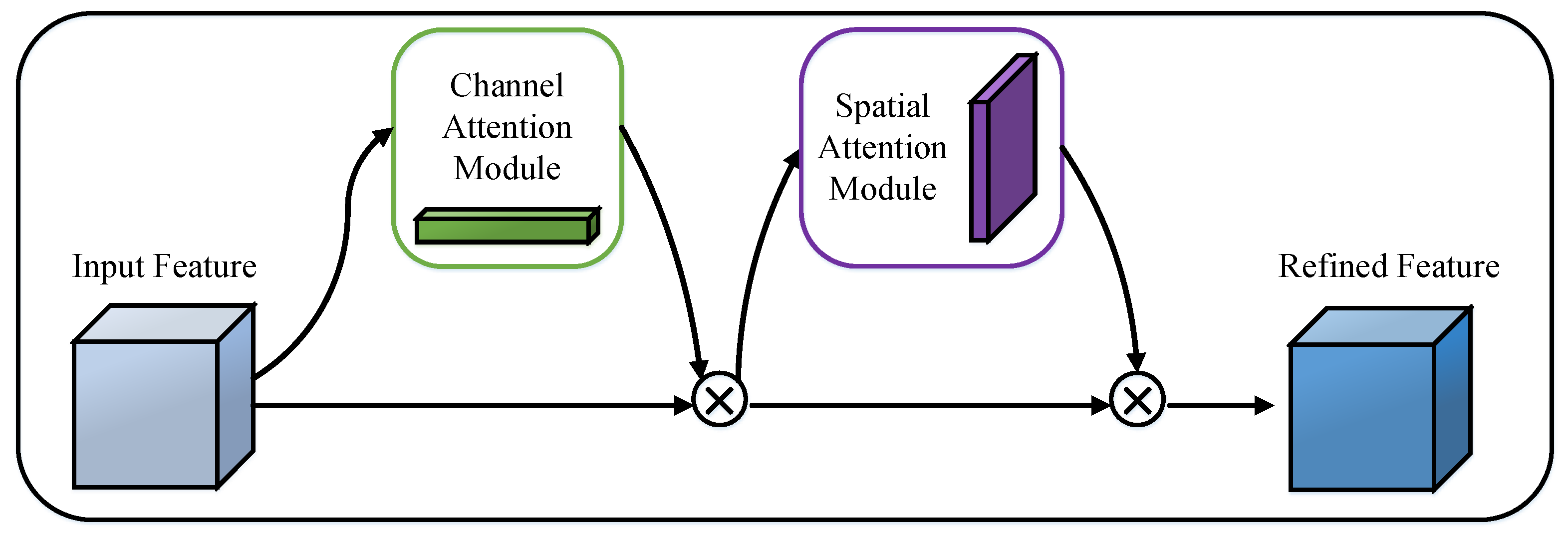
The convolutional block attention module (CBAM) is lightweight compared to other attention modules. It consists of two attention modules in series, namely, the channel attention module and spatial attention module [44]. Figure 3 shows the network structure of the CBAM. In the process of image feature extraction, the CBAM adaptively calculates better weight values in the dimensions of channel and space so that important features can be fully utilized in the subsequent iterative learning of parameters. The learning process of the neural network is strengthened so that the identification model focuses more on features unique to the image [45].
The structure of the channel attention module is illustrated in Figure 4. First, assuming that the input feature map is F , it enters the max pooling layer and average pooling layer. Second, the derived features of the two pooling layers are input into the multilayer perceptron (MLP) to obtain new features. Third, two new features are added. Fourth, the sigmoid activation function is used to calculate the channel feature weight vector M C . Last, the original input feature F is multiplied by the channel feature weight to obtain the channel attention feature F , which is expressed as:
F = M C ( F ) F
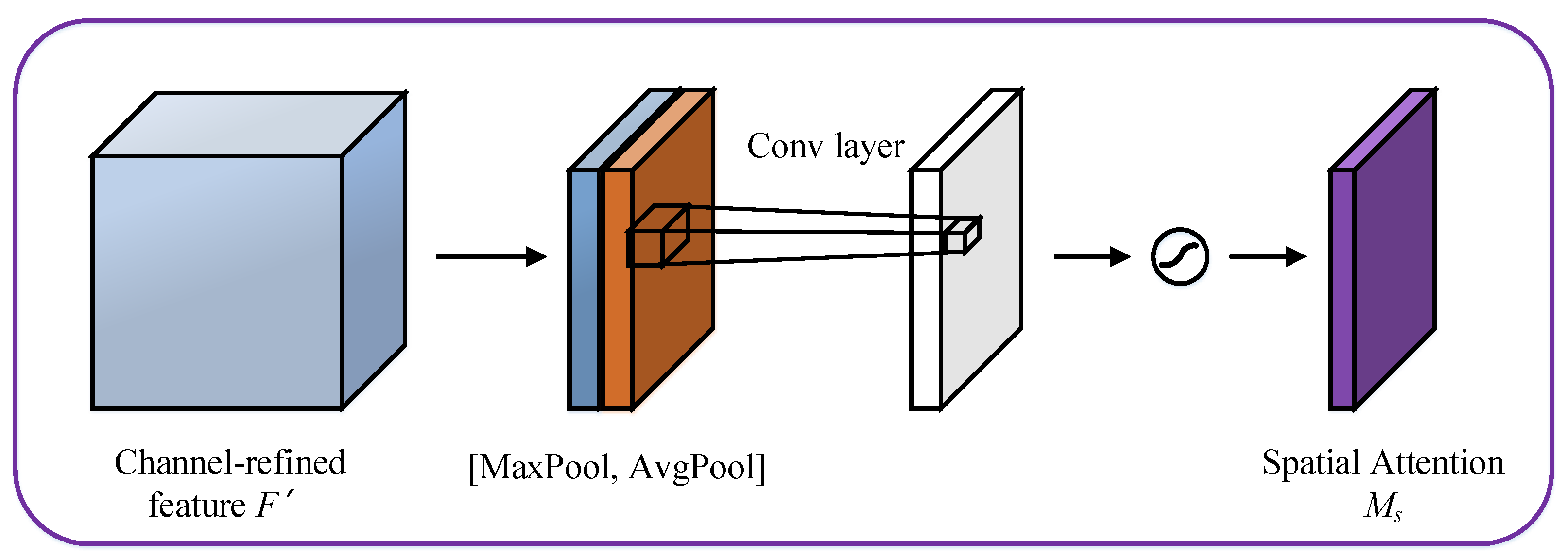
The structure of the spatial attention module is shown in Figure 5. The channel attention feature F obtained by the channel attention module serves as the input feature of the spatial attention module for the max pooling calculation and average pooling calculation. The derived results are spliced to obtain new features, and then the convolution operation is performed on this new feature. The size of the convolution kernel is 7 × 7, and the spatial weight vector M S is calculated by the sigmoid activation function. The spatial feature F is obtained by multiplying the spatial weight vector and channel feature by:
F = M S ( F ) F
where is elementwise multiplication. The channel attention module focuses on important features in the channel dimension of the feature map, while the spatial attention module focuses on important features in the spatial dimension. In both the channel attention module and spatial attention module, the input features are calculated by max pooling and average pooling.
The calculation relationship between the channel and the spatial weight vector is expressed as follows:
M C ( F ) = σ ( M L P ( A v g P o o l ( F ) + M L P ( M a x P o o l ( F ) ) )
M s ( F ) = σ ( C o n v ( [ A v g P o o l ( F ) ; M a x P o o l ( F ) ] ) )
where σ ( ) is the sigmoid activation function, M L P ( ) is a multilayer perceptron, A v g P o o l ( ) is the average pooling calculation, M a x P o o l ( ) is the max pooling calculation and C o n v ( ) is the two-dimensional convolution calculation.

2.2.2. ECA Mechanism

Efficient channel attention (ECA) is an optimization model of squeeze-and-excitation (SE) attention [46], which uses fewer parameters to enhance the performance of the model. ECA is also a plug-and-play attention mechanism module [47]. The forward flow of the ECA module is to perform global average pooling in different channel dimensions of the input feature map and then to splice it into a one-dimensional feature vector. Then, the new feature vector is convoluted by a one-dimensional convolution kernel, and the new weight value is calculated by the sigmoid activation function. The new features are calculated by multiplying by the original input features. The advantage of this calculation method is that it effectively avoids the problem of channel dimension reduction and enables cross-channel feature information interaction [48], thus achieving an efficient feature extraction process. Figure 6 shows the structure of the ECA module.
In the process of parameter learning, the ECA module shares the same learning parameters with all channels [49] and achieves efficient information cross-channel interaction. The process is expressed as follows:
ω i = σ ( j = 1 k ω j y i j ) , y i j Ω i k
Note that this parameter sharing process can be easily realized by using one-dimensional convolution with a convolution kernel size of k . The one-dimensional convolution process is expressed as follows:
ω = σ ( C 1 D k ( y ) )
where C 1 D ( ) is a one-dimensional convolution and σ ( ) is the sigmoid activation function. When using this method in the ECA module, only k parameters are involved.
In the process of using cross-channel information interaction to enhance the effect of feature extraction, it is necessary to determine the appropriate interaction coverage, that is, to determine the appropriate size of the one-dimensional convolution kernel [50]. In the CNN architecture, the output features of different locations often have different numbers of channels. If the optimal cross-channel interaction coverage suitable for different channel numbers is obtained by manually adjusting the size of the convolution kernel, the computational resources and time cost are considerable. Wang et al. proposed an adaptive convolution kernel size determination method that can be utilized in different channel dimensions [48]. Given the number of channels C , an adaptive one-dimensional convolution kernel size k is obtained. There is a mapping relationship between C and k :
C = ϕ ( k )
Linear function mapping, such as Equation (13), is a common and simple mapping relation. However, because linear mapping is too simple, it cannot meet the actual needs in many cases and will be subject to many restrictions. In CNN parameters, the channel dimension C is generally a power of 2. Therefore, the original linear function Equation (13) is improved to obtain a nonlinear mapping function, as shown in Equation (14).
ϕ ( k ) = γ × k b
C = ϕ ( k ) = 2 ( γ × k b )
The size of the one-dimensional convolution kernel k is determined by the number of channels C according to:
k = ψ ( C ) = log 2 ( C ) γ + b γ o d d
where t o d d is the odd number closest to t , γ is set to 2 and b is set to 1. According to the mapping relationship in Equation (15), it can be concluded that high-dimensional channels need to use larger convolution kernels to adapt to cross-channel interactions. In contrast, the low-dimensional channel determines a smaller convolution kernel to complete a shorter range of interactions.

2.3. Principle of CBAM-ECA-ResNet50

In summary, the convolutional layer in the network architecture of the deep learning CNN can quantify the features of the image by layer-by-layer advancement without the need to manually extract the unique features of the image. The introduction of an attention mechanism creates a new direction in improving the structure of the neural network and enhancing the performance of the model. Based on the classical network ResNet50, this study combines the two attention mechanism modules CBAM and ECA and adds them to the front and back positions of the four stages in ResNet50 (hereinafter referred to as the former position and the latter position). The aim is to improve the identification performance of the network model for gas–liquid two-phase flow patterns. According to the method and principle of model improvement, the proposed new model is defined and named CBAM-ECA-ResNet50. Figure 7 shows the network structure of CBAM-ECA-ResNet50. The collected gas–liquid two-phase flow pattern image data of the vertical pipeline are applied to the proposed model to realize the intelligent classification and identification process, which is mainly divided into four steps:
Step 1: The flow pattern image in the dataset is input into the model. First, the convolution layer and max pooling layer are passed in turn, and a preliminary feature map extraction is carried out to obtain feature maps with 64 channels. The max pooling layer has the effect of increasing the receptive field. The extracted preliminary features are input into the CBAM and then passed through the channel attention module and spatial attention module in the CBAM. The extracted preliminary features continue to calculate more appropriate weights in the dimensions of channel and space to further extract higher-quality remodeling features without changing the overall channel dimension.
Step 2: The reconstructed features enter an important part of ResNet50, a continuous convolution layer composed of 16 bottlenecks, which is divided into 4 stages. The number of channels output by each stage is 256, 512, 1024 and 2048. In this process, because of the unique residual mapping structure of ResNet50, the reconstructed features of CBAM output are further extracted.
Step 3: The new feature output at the end of the fourth stage will enter the ECA module to make the 2048-dimensional features fully undergo cross-channel information interaction so that the model pays more attention to the correlation among different channel features. Because the position of the ECA module in the network structure and the channel dimension of the input features have been determined, the cross-channel interaction coverage in the ECA module can be calculated by Equation (15); that is, the convolution kernel size of the adaptive one-dimensional convolution is k = 7 . In this part, the feature weights are further optimized without channel dimension reduction.
Step 4: The global average pooling operation is performed on the features output by the ECA module to obtain a 1 × 1 × 2048 feature vector. This process does not require learning updated weight parameters and reduces the risk of model overfitting. The process also better reflects the global information of features. To make the model adapt to the identification task of four types of gas–liquid two-phase flow patterns in this study, the feature vector is connected to a fully connected layer with four neurons. The 2048-dimensional feature is mapped into a four-dimensional feature vector. By the comparison of the classification score ratio, the category of the image data is determined. Intelligent identification of flow pattern images is realized.
The size and dimension of the input image data in the model are 224 × 224 × 3. Table 1 shows all the structural parameters in CBAM-ECA-ResNet50.

3. Validation of CBAM-ECA-ResNet50

3.1. Dataset and Data Augmentation

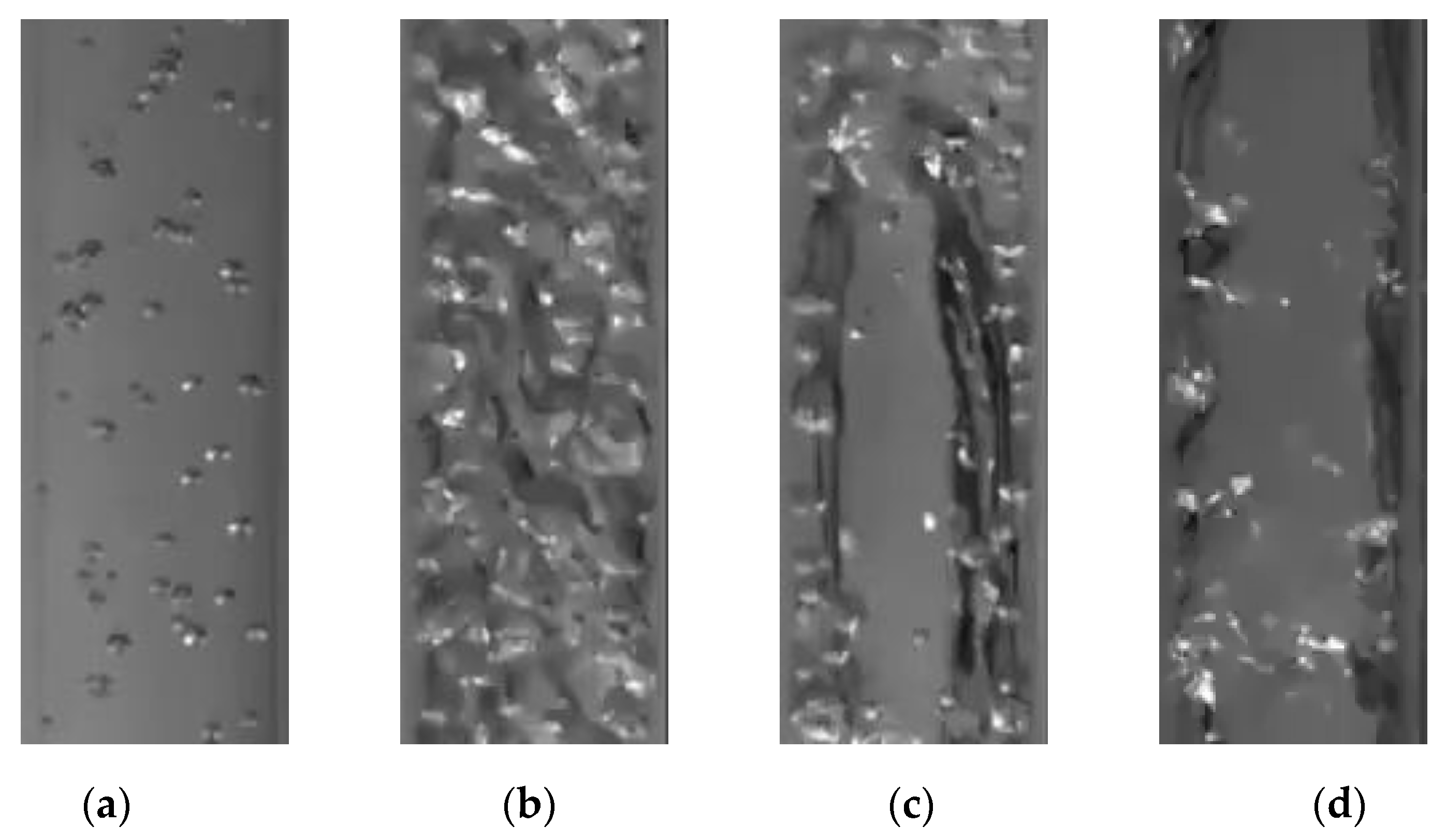
To validate the performance of the proposed new CBAM-ECA-ResNet50 for gas–liquid two-phase flow pattern identification, 3522 gas–liquid two-phase flow pattern images collected in the vertical pipeline are selected as the dataset of the model [51]. Labeling each image and using the method of no-return random sampling, with 70% as the training set and 30% as the validation set are shown in Table 2. Generally, due to the different flow rates of gas–liquid two-phases in the pipeline, the flow patterns of the fluid will also be different. The collected image data include four flow patterns, namely, sparse bubbly flow, dense bubbly flow, slug flow and annular flow. Sparse bubbly flow is one of the most common gas–liquid two-phase flow patterns in vertical pipelines and is characterized by bubbles of different sizes scattered in the liquid phase. Small bubbles are usually spherical, and larger bubbles may show different shapes. In dense bubbly flow, the velocity of bubbles is usually faster, the distribution of bubbles is diffuse and bubbles of different sizes are almost filled with the liquid phase. The bubble flow is theoretically divided into sparse bubbly flow and dense bubbly flow, which can be distinguished quantitatively by measurable parameters, such as bubble volume fraction, bubble diameter and bubble velocity. Generally, the bubbly flow with a bubble volume fraction below 0.1 and a bubble diameter less than 1 mm is identified as sparse bubbly flow; otherwise, it is the dense bubbly flow. As with the bubble velocity, in case of small bubble velocity, the flow pattern may be identified as sparse bubbly flow. However, in practice, there is no absolute criterion to distinguish sparse bubbly flow from dense bubbly flow due to the influence caused by various factors, such as pipe diameter and the relative volume fraction, diameter and velocity of the bubbles. In addition, in some cases, the dense bubbly flow can hardly be distinguished from slug flow by visual observation, which can be effectively solved by the model proposed in this study. When slug flow occurs in a vertical pipeline, the top phase boundary of the gas phase is usually arc-shaped. Thus, the slug flow in the vertical pipeline is sometimes referred to as plug flow, which is characterized by a large volume of gas phase gathered to form a gas slug. Gas slug and fluid in the liquid phase alternately appear in the pipeline. In industrial production, this flow pattern often produces a strong vibration in pipelines or related equipment [7,8], reducing its service life and increasing production costs. Therefore, accurate and efficient identification of slug flow has engineering significance. Annular flow generally occurs when the gas flow rate is large. The gas phase occupies the main body in the pipeline, and the liquid phase will be forced to fit on the inner wall of the pipeline to form a circular liquid film. Figure 8 shows the representative morphology of each flow pattern. In all image data, each image represents one of the flow patterns.
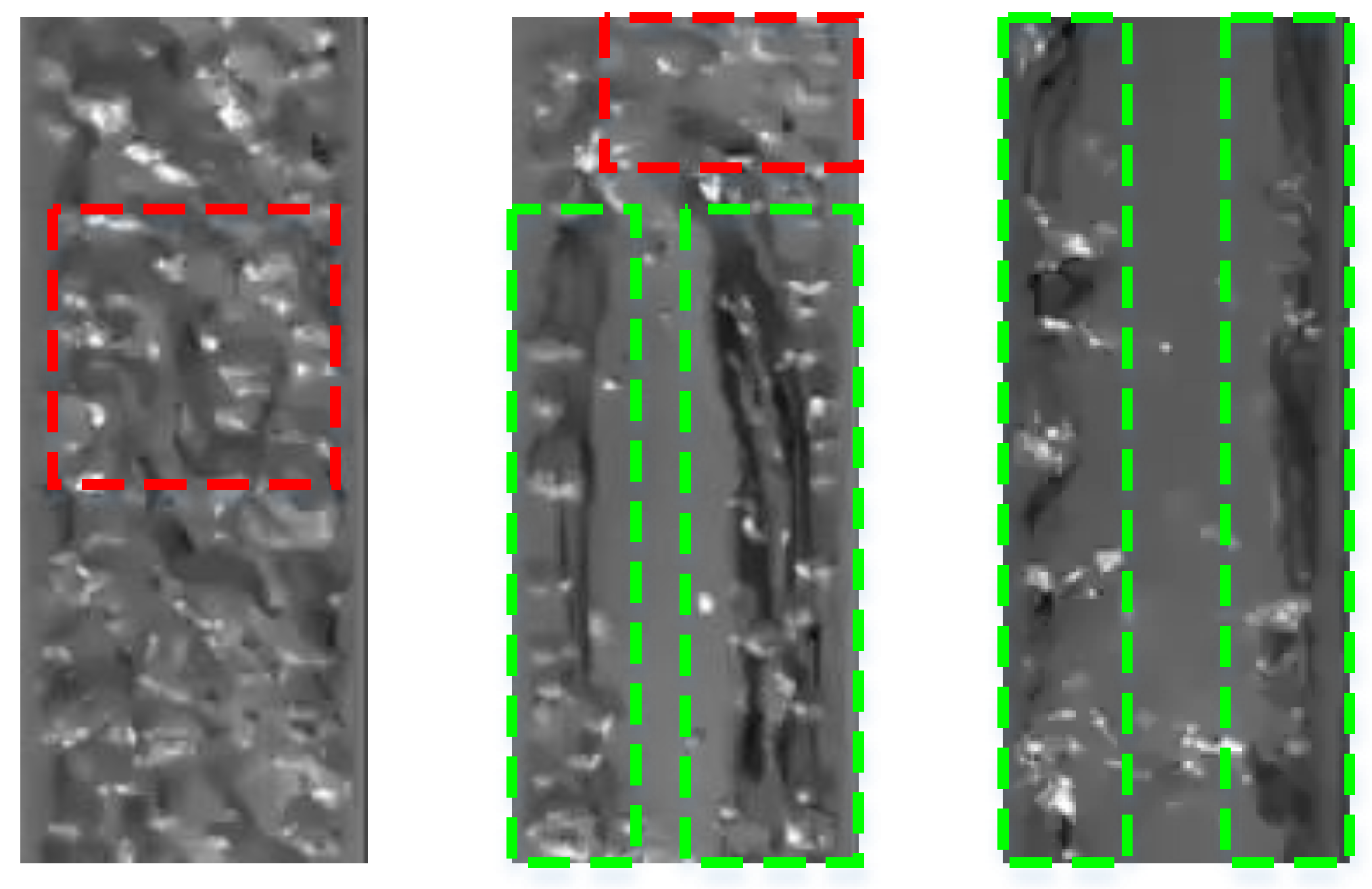
Although gas–liquid two-phase flow has a variety of flow patterns, there are also many similar features among the various patterns, which makes the flow pattern difficult to identify. If the flow pattern image is observed by the human eye to determine the type of flow pattern, it will be affected by human subjective ideas, especially when various flow patterns contain these similar features. This method is inefficient. Figure 9 shows similar features of different flow patterns. The red frame line represents high-density bubbles. Notably, both dense bubbly flow and slug flow have this feature. Therefore, when this feature appears in a large area, it will increase the difficulty of judging dense bubbly flow and slug flow. The slug part of slug flow, as shown in the green frame line, the vertical phase interface and the liquid film of the annular flow are also easily confused. When the slug length in the slug flow is relatively large, it is difficult to distinguish between slug flow and annular flow.
The neural network is in an underfitting state at the beginning of training. For certain practical tasks, the collection of datasets for training may be difficult, so there are insufficient data to help the neural network improve its ability to learn. Data augmentation technology can generate different data by fine-tuning the data, such as rotation, flipping, shape reshaping and masking. Strictly, the number of data samples does not increase, but because the data augmentation is random to each sample, the same original image data may exhibit different forms when entering the neural network, which indirectly increases the diversity of data features. In this study, a large amount of image data is generated by using the single sample data augmentation method of supervised learning. For the samples in the training set, the torchvision.transforms toolkit module in the PyTorch framework is introduced, and the RandomResizedCrop function is employed to randomly crop the image samples. Then, the cropped area image is scaled to a size of 224 × 224 × 3 by interpolation mapping. In this way, standard image data suitable for the model are generated. After adding the horizontal flip data augmentation operation, using the RandomFlip function, the value of flip_prob is set to 0.5. When the data are input into the model, there is a 50% probability that they will be horizontally flipped into new image data. Figure 10 shows the possible data augmentation pipeline in the training set. After conducting data augmentation on the dataset, the learning performance of the model is improved, and the generalization ability of the model identification is enhanced.
It should be noted that the collection of the dataset is not limited to the images being easily identified by the visual identification, but also images characterized by fuzzy features. In practice, however, the human subjective consciousness is able to classify the images with clear features into a certain flow pattern, and the discrimination of flow patterns for images with fuzzy features is often inefficient. In the present study, these images are also identified as one of the four flow patterns in the original data presentation. For instance, the captured slug flow images which have no clear gas–liquid interface or observable complete gas slug are indeed captured when the segmental slug flow phenomenon occurs in the pipeline. Considering the practical situation, the images with fuzzy features are also included in the dataset, which are assigned with lower weights when updating the model. Therefore, the flow pattern identification model proposed in this study cannot only identify specific flow patterns in batch and effectively, but also focuses on the fuzzy features corresponding to each flow pattern quantitatively as much as possible to improve the engineering values of the model. Specifically in the case of images being not discriminated by visual observation, the proposed model would give the most likely result based on deep learning.

3.2. Model Training

In the research of this study, a CNN model with a double attention mechanism module is constructed. To confirm that the identification performance of CBAM-ECA-ResNet50 is improved compared with that before the improvement, the new model CBAM-ECA-ResNet50 and the original model ResNet50 are used to train the prebuilt dataset. The parameter settings in the model are shown in Table 3. The optimizer is set to SGDM. To make the training process converge at a faster rate with greater stability, the momentum is set to 0.9. The weight decay (L2 regularization factor) is set to 0.0001. The purpose is to adjust the influence of model complexity on the loss function, effectively limit the range of network parameters and prevent the occurrence of model overfitting by penalizing the larger weight in the learning process. The initial learning rate is set to 0.1, and the learning rate is attenuated. Starting from the training starting point, every 30 epochs, the learning rate is attenuated to 0.1 times the original. The maximum number of epochs is 100 during training. The interpreter is Python 3.9 (Python Software Foundation, Amsterdam, Netherlands), and the PyTorch version is 1.10.0 (FAIR, Palo Alto, CA, USA). The device model used in the experiment is a single NVIDIA GeForce RTX3050 laptop GPU, VRAM 4G. In this study, the batch size of the model is 32.

3.3. Results and Model Performance Analysis

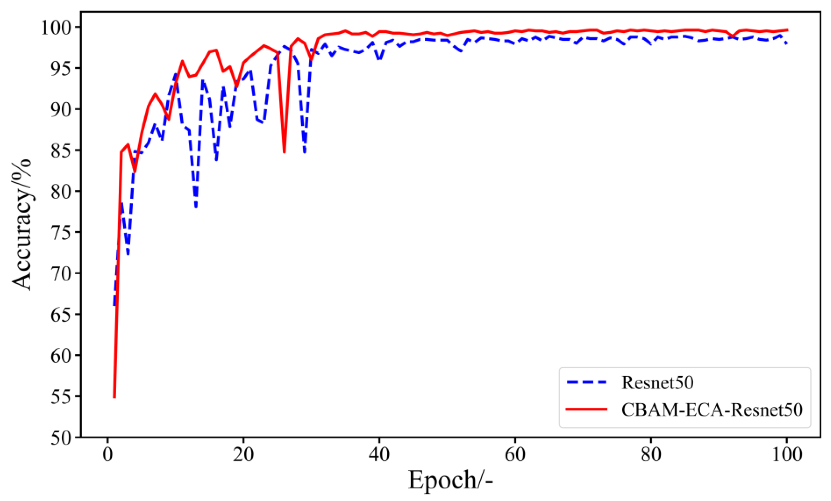
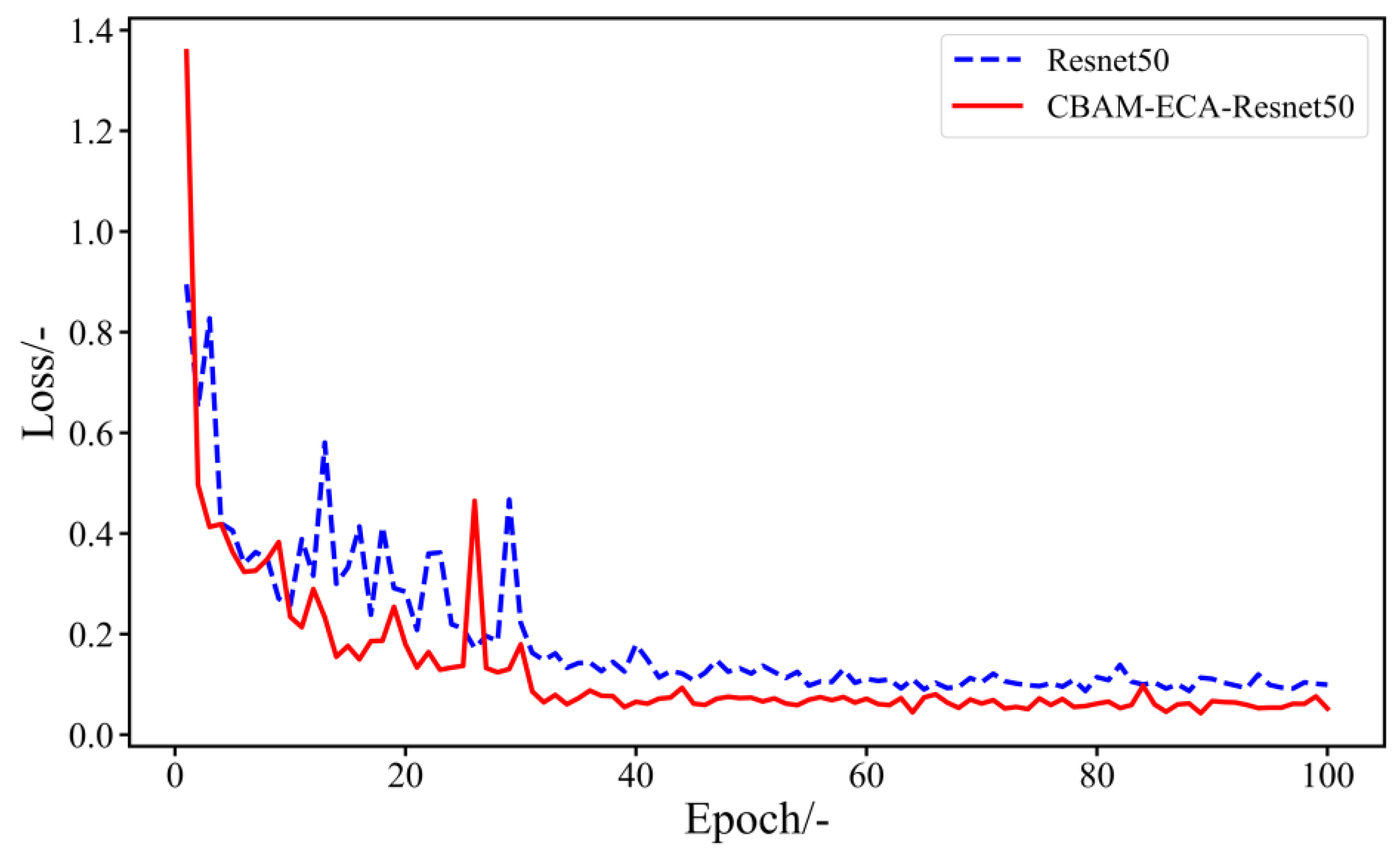
Since the proposed model is based on the classical model ResNet50, it is the most intuitive and convincing model to compare the performance of the improved model CBAM-ECA-ResNet50 with the original model. Figure 11 shows the change curve of the identification accuracy of CBAM-ECA-ResNet50 and ResNet50 on the validation set. Figure 12 shows the degree to which CBAM-ECA-ResNet50 and ResNet50 reduce the loss value of the validation set. These models have a common trend. After 30 epochs, the changes in accuracy and loss decline are more stable because at 31 epochs, the first attenuation of the learning rate occurs. The magnitude of each update parameter of the model begins to decline, which makes the process of model learning converge at a faster rate. While the weight parameters of the model are updated to the optimal weight at a faster speed, the weight update error caused by the large learning rate is avoided. During the training process of the model, we saved a set of weight parameters with the best identification effect of each model on the validation set. The identification accuracy of the original model ResNet50 for gas–liquid two-phase flow pattern image data is 98.96%. The proposed CBAM-ECA-ResNet50 increased the identification accuracy by 0.66% to 99.62%. The floating area of the accuracy is also higher than that of the ResNet50 model. CBAM-ECA-ResNet50 has a lower loss value of 0.05197 when identifying the validation set data. Compared with the original model, the loss value is reduced by 0.04927, which also shows that fewer images are misidentified. Higher identification accuracy and lower loss value provide cross-validation and data support for the proposed model with higher performance.
Since the two attention mechanism modules introduced in this study are plug and play, in theory, the positions of the attention mechanism can be exchanged with each other. Therefore, to verify the unique efficiency of the performance when the attention mechanism module is inserted into two specific positions, we use the CBAM and ECA module as the core to exchange the position order of the attention mechanism module. The number of attention mechanism modules changes, and multiple sets of different models with attention mechanism modules are constructed. The identification performance of these models for gas–liquid two-phase flow pattern image datasets was compared. Table 4 shows the simplified structure of the comparison model and describes the location and number of attention mechanism modules that were inserted.
The role of the attention mechanism is to attach a set of better weights to the existing features, thereby enhancing the features to a certain extent so that the model can learn better weight parameters. Therefore, in theory, the identification performance will improve after the attention mechanism module is introduced into the model. Even if the effect is not improved, it should not deteriorate. However, the calculation process of the neural network is a “black box” concept. The introduction of the attention mechanism may render the extracted feature weights too general and cannot be implemented on specific features, resulting in worse model performance. The position and number of attention mechanism modules may affect the identification effect of the model. In the comparative experiment of this study, Table 5 and Figure 13 show the identification effect of all the comparison models on the overall data of the validation set. In general, with the exception of CBAM-ECA-ResNet50, the identification accuracy of the other models with the CBAM decreased. However, the introduction of the ECA module improved the identification performance of the model in most cases.
This study inserts attention modules at two specific positions in the ResNet50 model. However, the number of input channels at these two positions is different. The input channel at the former position is 64 and that at the latter position is 2048. The two introduced attention mechanism modules have the function of further optimizing features in the channel dimension. However, the difference is that ECA can perform cross-channel information interaction on the channel dimension. Therefore, in theory, the ECA module can have a stronger channel feature information extraction function than CBAM. An analysis of the results in Table 5 and Figure 13 concluded that the identification effect of ResNet50-ECA is better than that of ECA-ResNet50 and ResNet50-CBAM and that the identification accuracy reaches 99.34%. This result further verifies that the ECA module will improve the performance of the model when it is inserted into a position with a larger number of input channels. In the same position with many channels, the ECA module improves the performance of the model more than CBAM. The influence of CBAM in different positions and different combinations on the performance of the model is unstable. However, under the condition that the ECA module is introduced at the latter position of the original model, the second attention module is introduced. The performance of CBAM-ECA-ResNet50 is better than that of ECA-ECA-ResNet50, and the identification accuracy is improved by 0.19%. This phenomenon shows that the channel dimension carries less feature information when the number of input channels is low. On the basis of ResNet50-ECA, the information interaction of the ECA module at low channel number positions has less influence on the performance improvement of the model in this experiment than the CBAM. Comparing all the experimental results, the identification accuracy of four combined models, which are CBAM-ECA-ResNet50, ECA-ECA-ResNet50, ECA-ResNet50 and ResNet50-ECA, is higher than that of the original model ResNet50. A common feature is that they all introduce the ECA module. However, after comparing ECA-CBAM-ResNet50, ECA-ECA-ResNet50 and ECA-ResNet50, it is concluded that only the performance of the ECA-CBAM-ResNet50 model is weaker than that of the original model ResNet50, and the identification accuracy is reduced by 0.48%. This finding shows that the feature extraction process of the CBAM in the latter position does not play a greater role and verifies that the ECA module performs more efficient weight optimization on the input features of the large channel in the latter position. Therefore, the combination and arrangement of attention in CBAM-ECA-ResNet50 is the best in the comparative experiment.
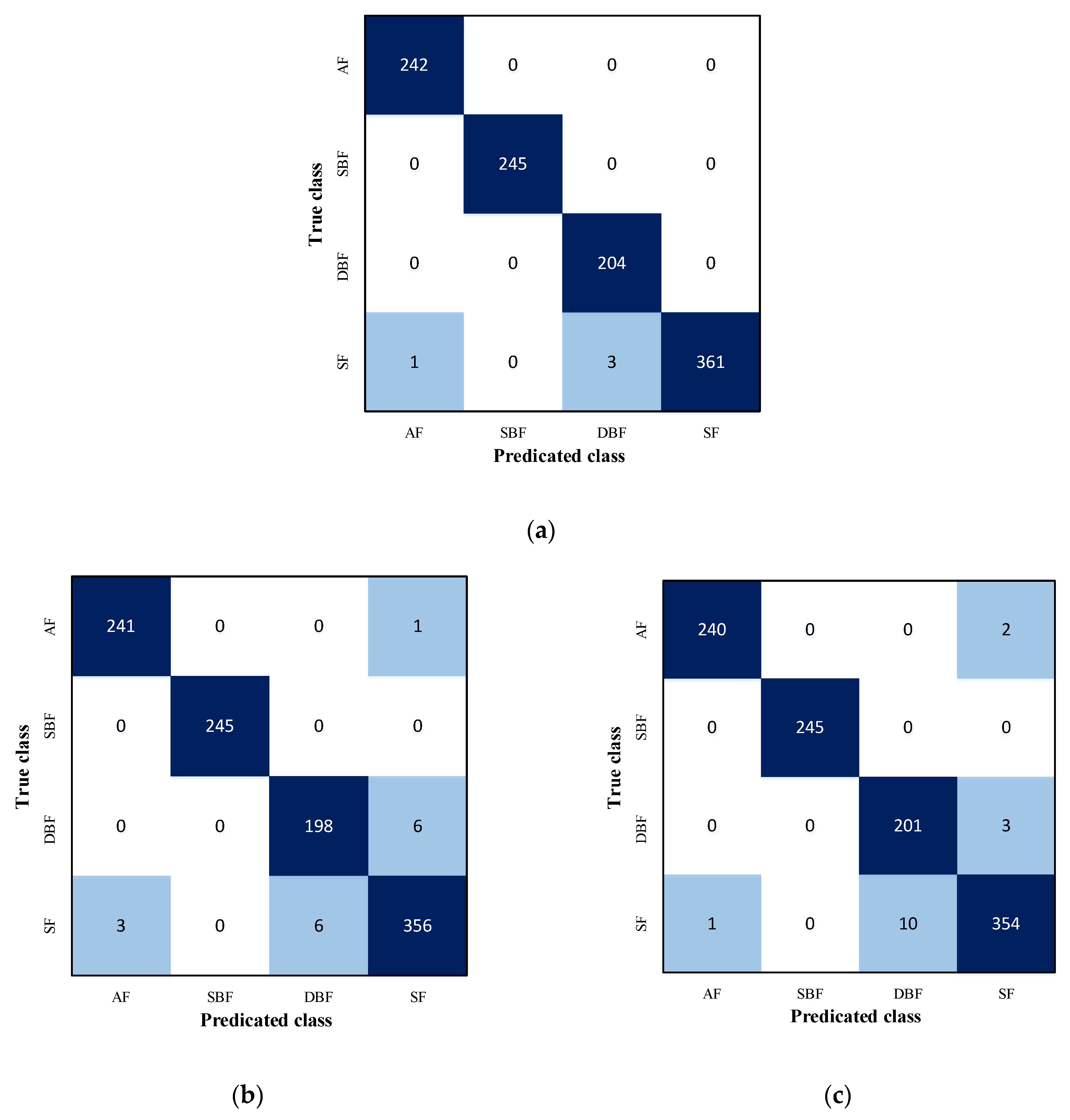
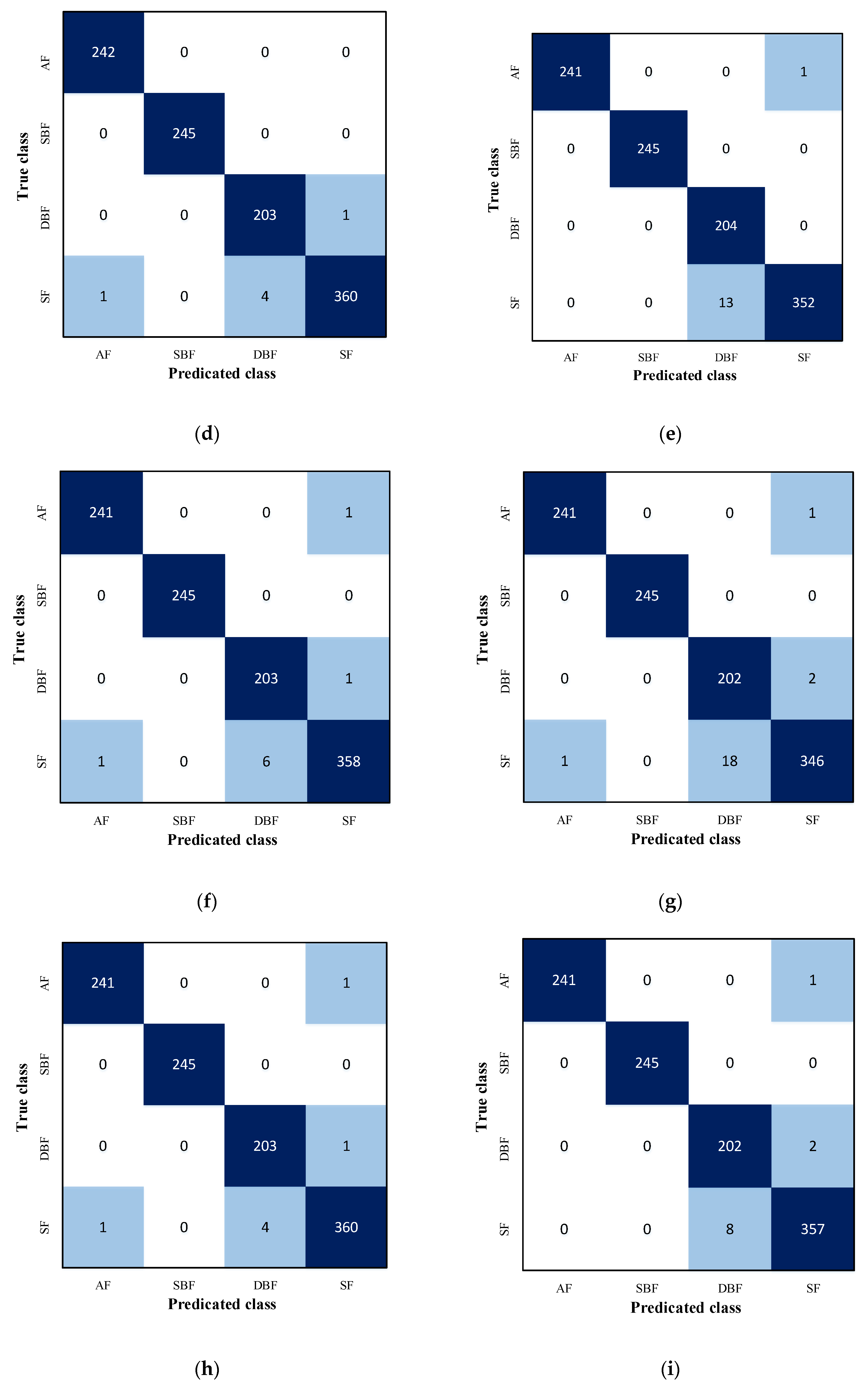
The role of the confusion matrix is different from the overall identification accuracy. The confusion matrix lists the prediction categories and error categories in the form of tables and specifically analyzes the identification of each type of image data. The matrix provides a more specific basis for discussing the identification results effect of the model. For the four labels, namely, annular flow (AF), sparse bubbly flow (SBF), dense bubbly flow (DBF) and slug flow (SF), the respective and average (AVG) precision, recall and F1 score are introduced, which provides a reference for evaluating the identification effect of the model on each class. Figure 14 shows the identification effect of the comparison model on the image data of the gas–liquid two-phase flow. The identification effect can be analyzed from the confusion matrix results:
(1)
Figure 14a–i show that all models correctly identify sparse bubbly flow. Table 6 shows that the precision, recall and F1 score of all models for sparse bubbly flow are 100%. The characteristics of sparse bubbly flow are the most obvious compared to other flow patterns.
(2)
In annular flow, one image is often mistakenly identified as slug flow. There are many bubbles in this annular flow image, so a similar phase interface appears in slug flow. However, both CBAM-ECA-ResNet50 and ECA-ECA-ResNet50 correctly classify this difficult annular flow image data, and the recall reached 100%. This finding shows that these two models enhance the process of feature extraction and improve the performance of model identification due to the introduction of an attention mechanism and realize the identification and classification of images with higher difficulty.
(3)
In contrast experiments, the error classification results are mostly concentrated in slug flow and dense bubbly flow because the slug flow in the dataset has different gas slug sizes and the image may be filled with foggy bubbles of different areas. These results are very similar to the characteristics of dense bubbly flow. The results of Figure 14a show that CBAM-ECA-ResNet50 only misclassifies slug flow and that the recall of slug flow is 98.90%. The other three types of image data are correctly classified, and the recall is 100%. Among the 365 slug flow images, only one image is misclassified as annular flow. The precision of CBAM-ECA-ResNet50 for annular flow is 99.59%, possibly because the gas slug in this slug flow image is too large, resulting in an increase in the void fraction of the pipeline in the instantaneous state and the formation of a long liquid film on the pipeline wall. Thus, the image features are similar to annular flow. In addition, three slug flow images were misclassified as dense bubbly flow. The classification results show that CBAM-ECA-ResNet50 has the best identification performance of gas–liquid two-phase flow pattern images in the comparison model.
(4)
Precision, recall and F1 score are important evaluation indicators for the model to identify each label datum. The precision, recall and F1 score of ResNet50-CBAM are the lowest: 97.64%, 98.35% and 97.95%, respectively. The precision, recall and F1 score of CBAM-ECA-ResNet50 are the highest: 99.54%, 98.90% and 99.63%, respectively. In a comprehensive comparison, CBAM-ECA-ResNet50, due to the introduction of the double attention modules, amplifies the important information in the feature map so that the iterative learning process of the model has been further optimized. Both the identification effect of the overall sample and the average classification effect index of specific categories are enhanced. The model has the best comprehensive performance in the comparison model.
Presently, a variety of attention modules rely on feature information in the channel dimension to optimize the weight parameters. In the process of forward propagation of image data, the number of feature map channels often changes. A larger number of channels means that more feature information is carried. Therefore, the attention mechanism module that optimizes the feature parameters in the channel dimension often plays a greater role in the position of a large channel number, which can more efficiently improve the overall performance of the model. We insert the lightweight attention module of channel attention evolution and an attention module of transformer architecture style into the latter position of the model, that is, the position with 2048 channels. In addition, we compare the impact on model performance and the change in model complexity. The complexity of the models and modules can be expressed by the parameter quantity and flops.
The ECA module in CBAM-ECA-ResNet50 was replaced with the SE, BAM, Shuffle and CoT modules. Table 7 shows the parameters of the model, the overall complexity of the model and the identification effect. Table 8 and Table 9 show the parameter quantity and flops for each part of the model. In different models, with the exception of the attention module, the complexity is the same. Most of the parameters are concentrated in four stages, and the number of parameters of the four stages increases in turn. The flops of the four stages also accounted this increase. Flops gradually increased from stage 1 to stage 3. In stage 4, although the number of channels in the feature map increases, the number of bottlenecks is only 3. The size of the feature map is 7 × 7, so the flops are reduced. In the 5 comparison models, the same input shape is determined to be 224 × 224 × 3, and the training parameter batch size is 32. ECA, SE, BAM and shuffle are lightweight attention mechanism modules, and the corresponding model size and flops are not very different. Compared with the original model ResNet50, the accuracy of the validation set of CBAM-BAM-ResNet50 and CBAM-Shuffle-ResNet50 is 97.92% and 98.67%, respectively, indicating that the BAM and shuffle attention module do not learn better weight parameters in the latter position. This results in reduced model performance and lower identification accuracy than the original model ResNet50. The identification accuracy of the validation set of CBAM-SE-ResNet50 is 99.43%, which is 0.47% higher than that of the original model. The SE attention module increases the channel weight of the input feature map and uses the full connection layer to extract the feature information in the channel dimension. Thus, the number of parameter quantities and flops are increased, reaching 24.045 M and 4.141 G, respectively. However, the increase is not large. The parameter quantity of the CBAM and SE modules accounted for 2.2%, and flops accounted for 0.386%. The ECA module uses a 1D convolutional layer instead of a fully connected layer to avoid the side effects of dimension reduction on channel attention. Adaptive methods are used to determine the size of the convolution kernel, which further improves the identification accuracy of CBAM-ECA-ResNet50, reaching 99.62%, which is 0.19% higher than that of CBAM-SE-ResNet50. Compared with CBAM-SE-ResNet50, the model size is reduced by 0.524 M, and flops are reduced by 0.001.
The CBAM-CoT-ResNet50 model introduces the CoT attention module. Due to the encoder process in the CoT module, the complexity of the model is greatly increased. The model size and flops reach 60.25 M and 5.94 G, respectively. The parameter quantity and flops of the CBAM and CoT module accounted for 60.969% and 30.556%, respectively. Although the complexity of the model greatly changed after the introduction of the CoT module, the CoT module did not achieve better performance due to the small amount of training data. The identification accuracy rate only reached 99.15%. The model performance was significantly weaker than that of CBAM-SE-ResNet50 and CBAM-ECA-ResNet50. If the amount of data is increased on the basis of existing conditions, the CBAM-CoT-ResNet50 model may have better identification results. A comprehensive comparison shows that under the existing experimental conditions, CBAM-ECA-ResNet50 has a relatively low model complexity and stronger performance in the gas–liquid two-phase flow pattern identification process.

3.4. Applicability Analysis

In this study, all the images used for the modeling of the flow pattern identification are all captured under the same illumination; as a result, the flow conditions and illumination are approximately the same. However, in case of different conditions, the proposed model may still be applicable or the applicability may be weakened to some extent, which can be improved by some existing techniques. Specifically, the situation beyond this study can be determined as the following two scenarios.
Scenario 1: The images used for flow pattern identification are the same and the illumination are different. In this case, the information associated with the interface between gas and liquid is affected to some extent by the illumination, and in the proposed model, this kind of information is critical for flow pattern identification. As a result, the accuracy of the proposed model may be affected by poor illumination due to the loss of some interface information. However, this issue can be solved satisfactorily by increasing the training dataset.
Scenario 2: The images and illumination used for the flow pattern identification are different from the dataset in this study. The identification capacity of the proposed model may be greatly weakened, which can be rectified by re-training and learning from the newly added image dataset to get a more adaptive and targeted flow pattern identification model.
Nevertheless, the above-mentioned issues can be solved as much as possible by taking some measures. For instance, the size of the dataset can be increased by adding data with different illumination and other widely varying data. In addition, other data enhancement methods can be integrated to increase the diversity of the data. In most cases, the models trained by such larger and more stylized datasets would be characterized by stronger generalization and robustness.

4. Conclusions

Based on the high efficiency of convolutional neural networks in the field of image recognition, this study uses the classical convolutional neural network ResNet50 as the basic architecture and introduces two attention mechanism modules. A more efficient intelligent identification method of the gas–liquid two-phase flow pattern is proposed. The CBAM and ECA mechanism module are added to two specific positions in ResNet50, and the number of neurons in the final fully connected layer is changed to four, corresponding to the four flow patterns in this research task. The effectiveness of the newly proposed CBAM-ECA-ResNet50 is verified by a dataset containing 3522 pictures of gas–liquid two-phase flow patterns in a vertical pipeline. To improve the identification accuracy and generalization ability of the model, data augmentation is used for the image data of the training set. Compared with the original ResNet50 model, the performance of the new model is fully improved. Then, the influence of the order and number of two attention mechanism modules, added to the specific position in ResNet50 on the performance of the model, is analyzed. The involved performance indicators are accuracy, precision, recall and F1 score. The other attention modules are introduced to compare the performance and complexity of the model. The comprehensive results show that CBAM-ECA-ResNet50 has better flow pattern identification performance.
This study provides guidance for the monitoring of multiphase flow in the process of oil-gas exploitation and gathering in the deep and far sea. This study only focuses on the identification of gas–liquid two-phase flow (actually, air–water two-phase flow) in vertical pipelines. Future research will expand the scope of research directions; increase the oil phase conditions; make the research conditions closer to the oil, gas and water multiphase flow in actual industrial production; and continue to explore a more powerful identification model to improve the ability of flow pattern identification in the production process of oil-gas fields. A real-time online monitoring system is developed to provide efficient guarantees for industrial production.

Author Contributions

Conceptualization and methodology, W.Q.; formal analysis, H.G.; resources, C.L.; data curation, E.H. and H.C. All authors have read and agreed to the published version of the manuscript.

Funding

This research was funded by Postdoctoral Funding of China, 2022M720626.

Institutional Review Board Statement

Not applicable.

Informed Consent Statement

Not applicable.

Data Availability Statement

The data presented in this study are available upon request from the corresponding author.

Conflicts of Interest

The authors declare no conflict of interest.

References

  1. Dalane, K.; Dai, Z.; Mogseth, G.; Hillestad, M.; Deng, L. Potential applications of membrane separation for subsea natural gas processing: A review. J. Nat. Gas Sci. Eng. 2017, 39, 101–117. [Google Scholar] [CrossRef]
  2. Kaushik, M.; Kumar, M. An alpha-cut interval based IF-importance measure for intuitionistic fuzzy fault tree analysis of subsea oil and gas production system. Appl. Ocean Res. 2022, 125, 103229. [Google Scholar] [CrossRef]
  3. Bhardwaj, U.; Teixeira, A.P.; Soares, C.G. Bayesian framework for reliability prediction of subsea processing systems accounting for influencing factors uncertainty. Reliab. Eng. Syst. Saf. 2022, 218, 108143. [Google Scholar] [CrossRef]
  4. Meribout, M.; Azzi, A.; Ghendour, N.; Kharoua, N.; Khezzar, L.; AlHosani, E. Multiphase Flow Meters Targeting Oil & Gas Industries. Measurement 2020, 165, 108111. [Google Scholar]
  5. Wang, H.; Xu, Y.; Shi, B.; Zhu, C.; Wang, Z. Optimization and intelligent control for operation parameters of multiphase mixture transportation pipeline in oilfield: A case study. J. Pipeline Sci. Eng. 2021, 1, 367–378. [Google Scholar] [CrossRef]
  6. Matsubara, H.; Naito, K. Effect of liquid viscosity on flow patterns of gas-liquid two-phase flow in a horizontal pipe. Int. J. Multiph. Flow 2011, 37, 1277–1281. [Google Scholar] [CrossRef]
  7. Kumar, S.; Kumar, S.; Kumar, I. Internal two-phase flow induced vibrations: A review. Cogent Eng. 2022, 9, 2083472. [Google Scholar]
  8. Khan, U.; Pao, W.; Sallih, N. A review: Factors affecting internal two-phase flow-induced vibrations. Appl. Sci. 2022, 12, 8406. [Google Scholar] [CrossRef]
  9. Xue, Y.; Stewart, C.; Kelly, D.; Campbell, D.; Gormley, M. Two-Phase Annular Flow in Vertical Pipes: A Critical Review of Current Research Techniques and Progress. Water 2022, 14, 3496. [Google Scholar] [CrossRef]
  10. Besagni, G.; Varallo, N.; Mereu, R. Computational Fluid Dynamics Modelling of Two-Phase Bubble Columns: A Comprehensive Review. Fluids 2023, 8, 91. [Google Scholar] [CrossRef]
  11. Li, L.; Dong, F.; Zhang, S. Adaptive spatio-temporal feature extraction and analysis for horizontal gas-water two-phase flow state prediction. Chem. Eng. Sci. 2023, 268, 118434. [Google Scholar] [CrossRef]
  12. Tang, T.; Yang, J.; Zheng, J.; Wong, L.; He, S.; Ye, J.; Ou, G.F. Failure analysis and prediction of pipes due to the interaction between multiphase flow and structure. Eng. Failure Anal. 2009, 16, 1749–1756. [Google Scholar] [CrossRef]
  13. Wiedemann, P.; Doss, A.; Schleicher, E.; Hampel, U. Fuzzy flow pattern identification in horizontal air-water two-phase flow based on wire-mesh sensor data. Int. J. Multiph. Flow 2019, 117, 153–162. [Google Scholar] [CrossRef]
  14. Nie, F.; Wang, H.; Song, Q.; Zhao, Y.; Shen, J.; Gong, M. Image identification for two-phase flow patterns based on CNN algorithms. Int. J. Multiph. Flow 2022, 152, 104067. [Google Scholar] [CrossRef]
  15. Quero, G.; Mascagni, P.; Kolbinger, F.R.; Fiorillo, C.; De Sio, D.; Longo, F.; Schena, C.A.; Laterza, V.; Rosa, F.; Menghi, R.; et al. Artificial Intelligence in Colorectal Cancer Surgery: Present and Future Perspectives. Cancers 2022, 14, 3803. [Google Scholar] [CrossRef]
  16. Guo, J.; Bai, L.; Yu, Z.; Zhao, Z.; Wan, B. An ai-application-oriented in-class teaching evaluation model by using statistical modeling and ensemble learning. Sensors 2021, 21, 241. [Google Scholar] [CrossRef]
  17. Xie, J.; Zheng, Y.; Du, R.; Xiong, W.; Cao, Y.; Ma, Z.; Cao, D.; Guo, J. Deep Learning-Based Computer Vision for Surveillance in ITS: Evaluation of State-of-the-Art Methods. IEEE Trans. Veh. Technol. 2021, 70, 3027–3042. [Google Scholar] [CrossRef]
  18. Huang, Y.; Li, D.; Niu, H.; Conte, D. Visual identification of oscillatory two-phase flow with complex flow patterns. Measurement 2021, 186, 110148. [Google Scholar] [CrossRef]
  19. Du, M.; Yin, H.; Chen, X.; Wang, X. Oil-in-water two-phase flow pattern identification from experimental snapshots using convolutional neural network. IEEE Access 2019, 7, 6219–6225. [Google Scholar] [CrossRef]
  20. Zhang, L.; Wang, H.; He, Y.; Cui, Z. Two-Phase Flow Feature Extraction and Regime Identification in Horizontal Pipe. In Proceedings of the 2008 7th World Congress on Intelligent Control and Automation, Chongqing, China, 25–27 June 2008. [Google Scholar]
  21. Qi, G.; Dong, F.; Xu, Y.; Wu, M.; Hu, J. Gas/liquid two-phase flow regime identification in horizontal pipe using support vector machines. In Proceedings of the 2005 4th International Conference on Machine Learning and Cybernetics, Canton, China, 18–21 August 2005. [Google Scholar]
  22. Saito, Y.; Torisaki, S.; Miwa, S. Two-phase flow regime identification using fluctuating force signals under machine learning techniques. In Proceedings of the 2018 26th International Conference on Nuclear Engineering (ICONE), London, UK, 22–26 July 2018. [Google Scholar]
  23. Currie, G. Intelligent Imaging: Anatomy of Machine Learning and Deep Learning. J. Nucl. Med. Technol. 2019, 47, 273–281. [Google Scholar] [CrossRef]
  24. Dong, S.; Xia, Y.; Peng, T. Traffic identification model based on generative adversarial deep convolutional network. Ann. Telecommun. 2022, 77, 573–587. [Google Scholar] [CrossRef]
  25. Wang, H.; Hou, J.; Chen, N. A Survey of Vehicle Re-Identification Based on Deep Learning. IEEE Access 2019, 7, 172443–172469. [Google Scholar] [CrossRef]
  26. Yuan, C.; Xu, C.; Wang, T.; Liu, F.; Zhao, Z.; Feng, P.; Guo, J. Deep multi-instance learning for end-to-end person re-identification. Multimed. Tools Appl. 2018, 77, 12437–12467. [Google Scholar] [CrossRef]
  27. Shahin, A.I.; Guo, Y.; Amin, K.M.; Sharawi, A.A. White blood cells identification system based on convolutional deep neural learning networks. Comput. Meth. Program. Biomed. 2019, 168, 69–80. [Google Scholar] [CrossRef] [PubMed]
  28. Ran, X.; Xue, L.; Zhang, Y.; Liu, Z.; Sang, X.; He, J. Rock Classification from Field Image Patches Analyzed Using a Deep Convolutional Neural Network. Mathematics 2019, 7, 755. [Google Scholar] [CrossRef] [Green Version]
  29. Cheung, M.; Shi, J.; Wright, O.; Jiang, L.Y.; Liu, X.; Moura, J.M.F. Graph Signal Processing and Deep Learning: Convolution, Pooling, and Topology. IEEE Signal Proc. Magaz. 2020, 37, 139–149. [Google Scholar] [CrossRef]
  30. Xu, H.; Tang, T. Two-phase flow pattern online monitoring system based on convolutional neural network and transfer learning. Nucl. Eng. Technol. 2022, 54, 4751–4758. [Google Scholar] [CrossRef]
  31. Li, W.; Song, W.; Yin, G.; Ong, M.C.; Han, F. Flow regime identification in the subsea jumper based on electrical capacitance tomography and convolution neural network. Ocean Eng. 2022, 266, 113152. [Google Scholar] [CrossRef]
  32. Xu, H.; Tang, H.; Zhang, B.; Liu, Y. Identification of two-phase flow regime in the energy industry based on modified convolutional neural network. Prog. Nucl. Energy 2022, 147, 104191. [Google Scholar] [CrossRef]
  33. Niu, X.; Gao, Y.; Wang, R.; Du, M. Vertical Oil-in-Water Flow Pattern Identification with Deep CNN-LSTM Network. In Proceedings of the 2020 International Conference on Intelligent Computing and Human-Computer Interaction (ICHCI), Sanya, China, 4–6 December 2020. [Google Scholar]
  34. OuYang, L.; Jin, N.; Ren, W. A new deep neural network framework with multivariate time series for two-phase flow pattern identification. Exp. Syst. Appl. 2022, 205, 117704. [Google Scholar] [CrossRef]
  35. Carrasquilla, J.; Melko, R.G. Machine learning phases of matter. Nat. Phys. 2017, 13, 431–434. [Google Scholar] [CrossRef] [Green Version]
  36. Hu, Y.; Modat, M.; Gibson, E.; Li, W.; Ghavamia, N.; Bonmati, E.; Wang, G.; Bandula, S.; Moore, C.M.; Emberton, M.; et al. Weakly-supervised convolutional neural networks for multimodal image registration. Med. Image Anal. 2018, 49, 1–13. [Google Scholar] [CrossRef]
  37. Rehman, A.; Naz, S.; Razzak, M.I.; Hameed, I.A. Automatic Visual Features for Writer Identification: A Deep Learning Approach. IEEE Access 2019, 7, 17149–17157. [Google Scholar] [CrossRef]
  38. Vives-Boix, V.; Ruiz-Fernandez, D. Synaptic metaplasticity for image processing enhancement in convolutional neural networks. Neurocomputing 2021, 462, 534–543. [Google Scholar] [CrossRef]
  39. Xia, X.; Jiang, S.; Zhou, N.; Cui, J.; Li, X. Groundwater contamination source identification and high-dimensional parameter inversion using residual dense convolutional neural network. J. Hydrol. 2022, 617, 129013. [Google Scholar] [CrossRef]
  40. He, K.; Zhang, X.; Ren, S.; Sun, J. Deep Residual Learning for Image Recognition. In Proceedings of the 2016 IEEE Conference on Computer Vision and Pattern Recognition (CVPR), Las Vegas, NV, USA, 27–30 June 2016. [Google Scholar]
  41. Yu, H.; Sun, H.; Tao, J.; Qin, C.; Xiao, D.; Jin, Y.; Liu, C. A multi-stage data augmentation and AD-ResNet-based method for EPB utilization factor prediction. Autom. Constr. 2023, 147, 104734. [Google Scholar] [CrossRef]
  42. Guo, M.; Xu, T.; Liu, J.; Liu, Z.; Jiang, P.; Mu, T.; Zhang, S.; Martin, R.R.; Cheng, M.; Hu, S. Attention mechanisms in computer vision: A survey. Comput. Vis. Media 2022, 8, 331–368. [Google Scholar] [CrossRef]
  43. Cai, S.; Wang, C.; Ding, J.; Yu, J.; Fan, J. FDAM: Full-dimension attention module for deep convolutional neural networks. Int. J. Multimed. Inf. Retr. 2022, 11, 599–610. [Google Scholar] [CrossRef]
  44. Huang, J.; Mo, J.; Zhang, J.; Ma, X. A Fiber Vibration Signal Recognition Method Based on CNN-CBAM-LSTM. Appl. Sci. Basel 2022, 12, 8478. [Google Scholar] [CrossRef]
  45. Woo, S.H.; Park, J.; Lee, J.Y.; Kweon, I.S. CBAM: Convolutional Block Attention Module. In Proceedings of the 15th European Conference on Computer Vision (ECCV), Munich, Germany, 8–14 September 2018. [Google Scholar]
  46. Hu, J.; Shen, L.; Albanie, S.; Sun, G.; Wu, E. Squeeze-and-Excitation Networks. IEEE Trans. Pattern Anal. Mach. Intell. 2020, 42, 2011–2023. [Google Scholar] [CrossRef] [Green Version]
  47. Shu, X.; Chang, F.; Zhang, X.; Shao, C.; Yang, X. ECAU-Net: Efficient channel attention U-Net for fetal ultrasound cerebellum segmentation. Biomed. Signal Proc. Control 2022, 75, 103528. [Google Scholar] [CrossRef]
  48. Wang, Q.; Wu, B.; Zhu, P.; Li, P.; Zuo, W.; Hu, Q. ECA-Net: Efficient Channel Attention for Deep Convolutional Neural Networks. In Proceedings of the 2020 IEEE/CVF Conference on Computer Vision and Pattern Recognition (CVPR), Seattle, WA, USA, 13–19 June 2020. [Google Scholar]
  49. Shi, Y.; Wang, Z.; Du, X.; Ling, G.; Jia, W.; Lu, Y. Research on the membrane fouling diagnosis of MBR membrane module based on ECA-CNN. J. Environ. Chem. Eng. 2022, 10, 107649. [Google Scholar] [CrossRef]
  50. Lin, X.; Huang, Q.; Huang, W.; Tan, X.; Fang, M.; Ma, L. Single Image Deraining via detail-guided Efficient Channel Attention Network. Comput. Graph. UK 2021, 97, 117–125. [Google Scholar] [CrossRef]
  51. Shaban, H.; Tavoularis, S. Video: Zorbubbles (Producing flow regimes in air-water flow). In Proceedings of the 68th Annual Meeting of the APS Division of Fluid Dynamics, Boston, MA, USA, 22–24 November 2015. [Google Scholar] [CrossRef]
Figure 1. ResNet50 network structure.
Jmse 11 00793 g001
Figure 2. Identity mapping block structure.
Jmse 11 00793 g002
Figure 3. CBAM structure.
Jmse 11 00793 g003
Figure 4. Channel attention module structure.
Jmse 11 00793 g004
Figure 5. Spatial attention module structure.
Jmse 11 00793 g005
Figure 6. ECA module structure.
Jmse 11 00793 g006
Figure 7. CBAM-ECA-ResNet50 structure.
Jmse 11 00793 g007
Figure 8. Gas–liquid two-phase flow patterns in the vertical pipeline. (a) Sparse bubbly flow; (b) dense bubbly flow; (c) slug flow; (d)annular flow.
Jmse 11 00793 g008
Figure 9. Similar features of different flow patterns.
Jmse 11 00793 g009
Figure 10. Data augmentation pipeline of the training dataset.
Jmse 11 00793 g010
Figure 11. Accuracy curve of the validation dataset.
Jmse 11 00793 g011
Figure 12. Loss value curve of the validation dataset.
Jmse 11 00793 g012
Figure 13. Identification accuracy of different models.
Jmse 11 00793 g013
Figure 14. Flow pattern classification results of different models. (a) Classification on results of CBAM-ECA-ResNet50; (b) classification on results of ECA-CBAM- ResNet50; (c) classification on results of CBAM-CBAM-ResNet50; (d) classification on results of ECA-ECA-ResNet50; (e) classification on results of CBAM-ResNet50; (f) classification on results of ECA-ResNet50; (g) classification on results of ResNet50-CBAM; (h) classification on results of ResNet50-ECA; (i) classification on results of ResNet50.
Jmse 11 00793 g014aJmse 11 00793 g014b
Table 1. CBAM-ECA-ResNet50 structure and related parameters.
PartLayer NameOutput SizeOperatorChannels
1Conv112 × 112conv7 × 764
2Max Pooling112 × 112max pool3 × 3-
3CBAM112 × 112channel attention module
spatial attention module
64
64
4Conv Stage 156 × 56 conv 1 × 1 conv 3 × 3 conv 1 × 1 × 3 64
64
256
5Conv Stage 228 × 28 conv 1 × 1 conv 3 × 3 conv 1 × 1 × 4 128
128
512
6Conv Stage 314 × 14 conv 1 × 1 conv 3 × 3 conv 1 × 1 × 6 256
256
1024
7Conv Stage 47 × 7 conv 1 × 1 conv 3 × 3 conv 1 × 1 × 3 512
512
2048
8ECA7 × 7ECA attention module2048
9Global Average Pooling1 × 1global average pool-
10Fully Connected1 × 1fully connected4
11Output
Table 2. Statistics of flow pattern datasets.
ClassificationOriginal DatasetTraining DatasetValidation Dataset
Annular flow807565242
Sparse bubbly flow818573245
Dense bubbly flow681477204
Slug flow1216851365
Total352224661056
Table 3. Setting of model training parameters.
Parameters
OptimizerSGDM
Momentum0.9
Weight decay0.0001
Initial learning rate0.1
Learning rate decay step30/60/90 (Epoch)
Decay rate0.1
Batch size32
Max epoch100
Table 4. Comparative models of attention modules in different positions.
Model NameNumber of Attention ModulesSimplified Structure of the Model
ECA-CBAM-Resnet502Jmse 11 00793 i001
CBAM-CBAM-ResNet502Jmse 11 00793 i002
ECA-ECA-ResNet502Jmse 11 00793 i003
CBAM-Resnet501Jmse 11 00793 i004
ECA-Resnet501Jmse 11 00793 i005
Resnet50-CBAM1Jmse 11 00793 i006
Resnet50-ECA1Jmse 11 00793 i007
Table 5. Relevant parameters and identification accuracy of the model.
ModelsImage SizeBatch SizeMemory/MbLossValidation
Accuracy/%
CBAM-ECA-ResNet502243230140.0519799.62 (↑)
ECA-CBAM-ResNet502243229930.1129298.48 (↓)
CBAM-CBAM-ResNet502243230200.1113698.48 (↓)
ECA-ECA-ResNet502243229880.0625099.43 (↑)
CBAM-ResNet502243230180.0943698.67 (↓)
ECA-ResNet502243229920.0848199.15 (↑)
ResNet50-CBAM2243229690.0960398.67 (↓)
ResNet50-ECA2243229630.0623999.34 (↑)
ResNet502243229670.1012498.96
(↑) represents an increase in accuracy. (↓) represents a decrease in accuracy.
Table 6. Precision, recall and F1 score of the models.
ModelsPrecision/%Recall/%F1 Score/%
AFSBFDBFSFAVGAFSBFDBFSFAVGAFSBFDBFSFAVG
CBAM-ECA-ResNet5099.5910098.5510099.5410010010098.9099.7399.7910099.2799.4599.63
ECA-CBAM-ResNet5098.7710097.0698.0798.4899.5910097.0697.5398.5599.1810097.0697.8098.51
CBAM-CBAM-ResNet5099.5910095.2698.6198.3799.1710098.5396.9998.6799.3810096.8797.8098.51
ECA-ECA-ResNet5099.5910098.0799.7299.3510010099.5198.6399.5499.7910098.7899.1799.44
CBAM-ResNet5010010094.0199.7298.4399.5910010096.4499.0199.7910096.9198.0598.69
ECA-ResNet5099.5910097.1399.4499.0499.5910099.5198.0899.3099.5910098.3198.7699.16
ResNet50-CBAM99.5910091.8299.1497.6499.5910099.0294.7998.3599.5910095.2896.9297.95
ResNet50-ECA99.5910098.0799.4599.2899.5910099.5198.6399.4399.5910098.7899.0499.35
ResNet5010010096.1999.1798.8499.5910099.0297.8199.1199.7910097.5898.4998.97
Precision = TP/(TP + FP). Recall = TP/(TP + FN). F1 score = 2 × Precision × Recall/(Precision + Recall). TP, true positive; FP, false positive; TN, true negative; FN, false negative.
Table 7. Parameters and results of different attention combinations.
ModelsInput ShapeBatch SizeModel SizeFlopsValidation Accuracy/%
CBAM-ECA-ResNet50(224, 224, 3)3223.521 M4.140 G99.62 (↑)
CBAM-SE-ResNet50(224, 224, 3)3224.045 M4.141 G99.43 (↑)
CBAM-BAM-ResNet50(224, 224, 3)3224.787 M4.159 G97.92 (↓)
CBAM-Shuffle-ResNet50(224, 224, 3)3223.521 M4.140 G98.67 (↓)
CBAM-CoT-ResNet50(224, 224, 3)3260.250 M5.940 G99.15 (↑)
(↑) represents an increase in accuracy. (↓) represents a decrease in accuracy.
Table 8. Parameter quantity and overall proportion of each part of the different models.
ModelsParameter Quantity and Proportion
Conv + Max PoolingConv Stage 1Conv Stage 2Conv Stage 3Conv Stage 4Attention ModulesGAP + FC
CBAM-ECA-ResNet500.009 M0.216 M1.220 M7.098 M14.965 M0.005 M0.008 M
0.038%0.918%5.187%30.177%63.624%0.021%0.034%
CBAM-SE-ResNet500.009 M0.216 M1.220 M7.098 M14.965 M0.529 M0.008 M
0.037%0.898%5.074%29.520%62.237%2.200%0.033%
CBAM-BAM-ResNet500.009 M0.216 M1.220 M7.098 M14.965 M1.271 M0.008 M
0.036%0.871%4.922%28.636%60.374%5.128%0.032%
CBAM-Shuffle-ResNet500.009 M0.216 M1.220 M7.098 M14.965 M0.005 M0.008 M
0.038%0.918%5.187%30.177%63.624%0.021%0.034%
CBAM-CoT-ResNet500.009 M0.216 M1.22 M7.098 M14.965 M36.734 M0.008 M
0.015%0.359%2.025%11.781%24.838%60.969%0.013%
Table 9. Flops and overall proportion of each part of different models.
ModelsFlops and Proportion
Conv + Max PoolingConv Stage 1Conv Stage 2Conv Stage 3Conv Stage 4Attention ModulesGAP + FC
CBAM-ECA-ResNet500.122 G0.680 G1.037 G1.471 G0.811 G0.015 G0.004 G
2.947%16.425%25.048%35.531%19.589%0.362%0.097%
CBAM-SE-ResNet500.122 G0.680 G1.037 G1.471 G0.811 G0.016 G0.004 G
2.946%16.421%25.042%35.523%19.585%0.386%0.097%
CBAM-BAM-ResNet500.122 G0.680 G1.037 G1.471 G0.811 G0.034 G0.004 G
2.933%16.350%24.934%35.369%19.500%0.818%0.096%
CBAM-Shuffle-ResNet500.122 G0.680 G1.037 G1.471 G0.811 G0.015 G0.004 G
2.947%16.425%25.048%35.531%19.589%0.362%0.097%
CBAM-CoT-ResNet500.122 G0.680 G1.037 G1.471 G0.811 G1.815 G0.004 G
2.054%11.448%17.458%24.764%13.653%30.556%0.067%
Disclaimer/Publisher’s Note: The statements, opinions and data contained in all publications are solely those of the individual author(s) and contributor(s) and not of MDPI and/or the editor(s). MDPI and/or the editor(s) disclaim responsibility for any injury to people or property resulting from any ideas, methods, instructions or products referred to in the content.