Cost–Benefit Analysis of a Trans-Arctic Alternative Route to the Suez Canal: A Method Based on High-Fidelity Ship Performance, Weather, and Ice Forecast Models

Abstract

Climate change in recent years has produced viable shipping routes in the Arctic. However, critical uncertainties related to maritime operations in the Arctic make it difficult to predict ship speeds in ice and, thus, the voyage time and fuel costs. Cost–benefit analysis of alternative Arctic routes based on accurate environmental condition modeling is required. In this context, this paper presents a holistic approach that considers the major voyage-related costs of a trans-Arctic route as an alternative to the conventional routes via the Suez Canal Route (SCR) for existing merchant ships. This tool is based on high-fidelity models of ship performance, metocean forecasting, and a voyage optimization algorithm. Case studies are performed based on a general cargo vessel in operation to quantify realistic expenses inclusive of all the major operational, fuel, and voyage costs of the specific voyages. A comparison is made between the total costs of the trans-Arctic route and SCR for different seasons, which proves the economic feasibility of the trans-Arctic route. Overall, this work can provide valuable insights to help policymakers as well as shipbuilders, owners, and operators to assess the potential cost-effectiveness and sustainability of future Arctic shipping, thereby better developing future strategies.

1. Introduction

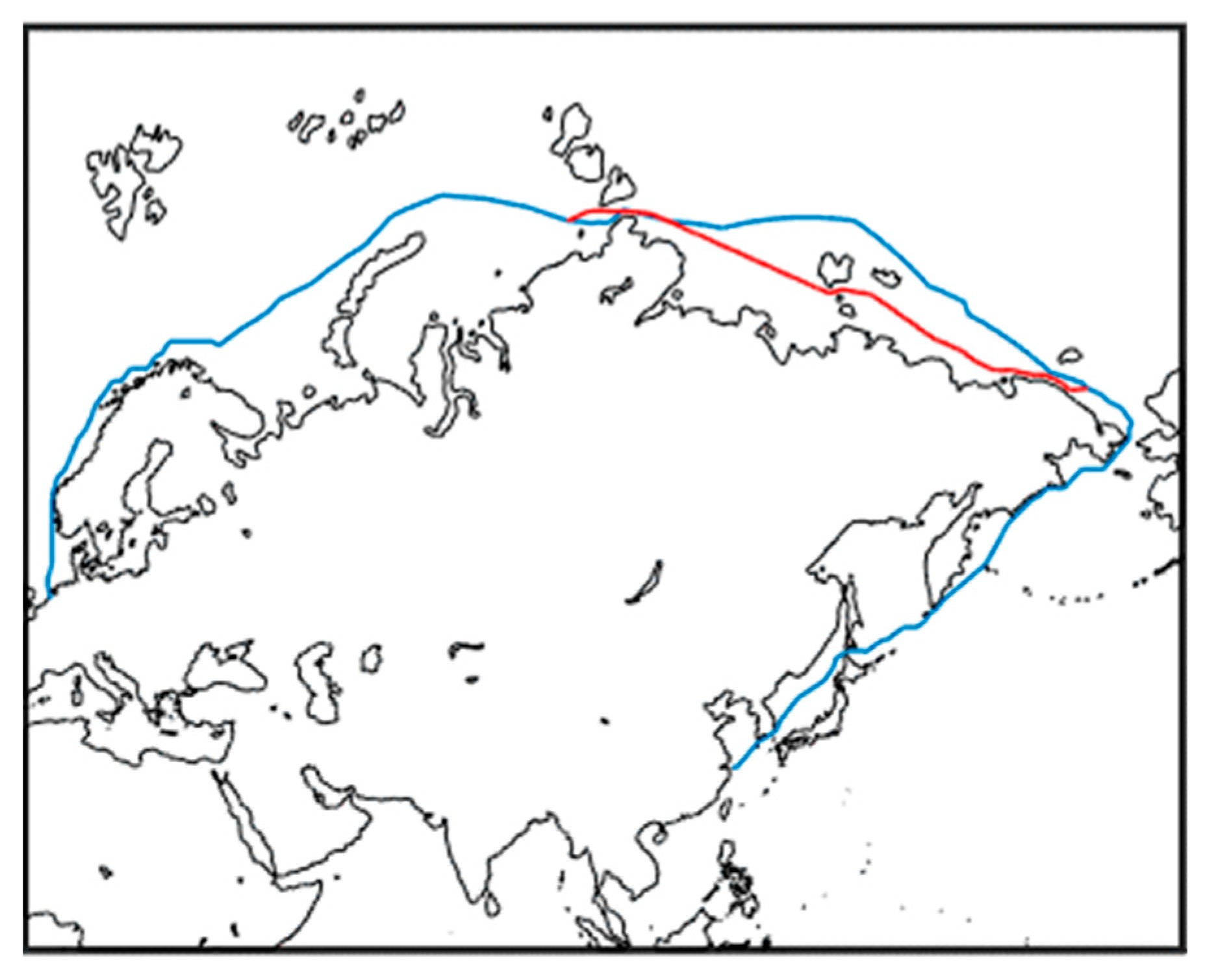
From 23 to 29 March 2021, the Ever Given containership blocked the Suez Canal, as shown in Figure 1. This blockage caused 369 ships to queue, and approximately 12% of global trade was delayed. Some vessels were rerouted to avoid the Suez Canal, which added approximately eight days to their total journeys and considerable additional fuel costs. The direct economic cost was over USD 10 billion, and the continuous cost is expected to exceed USD 100 billion [1]. This disastrous event reminds the public of the closure of the Suez Canal after the 1967 Six-Day War. During the closure period of 1967–1975, ships sailing between Europe and Asia had to take the much longer route around the Cape of Good Hope. Research shows that this increase in sea distance had marked negative impacts on world trade [2]. The Ever Given incident highlights once more the necessity of developing an alternative sea route to the Suez Canal, which must have competitive voyage-related costs.

The Northern Sea Route (NSR) that passes through the Arctic Sea is now a promising candidate for such an alternative route [3]. As a consequence of climate change, the NSR, which was previously covered by ice year-round, is already navigable for commercial vessels for over 100 days per year, and this number is still increasing [4,5]. The NSR has approximately 40% shorter lengths between major ports in Europe and Asia compared to the Suez Canal Route (SCR). However, the shorter distance by itself is not sufficiently attractive for ship owners. In 2019–2021, a total of 37, 64, and 85 transit voyages were conducted through the NSR, respectively [6]. For the same years, approximately 18–20,000 ships passed through the SCR [7], or an average of 50~55 passages per day. These passages can hardly be explained by the limited navigation season of the NSR, which is between four and five months [4]. Instead, these passages are an indication that the majority of shipping companies are skeptical about the overall cost competitiveness of the NSR.

Many studies of the economic feasibility of the NSR compared to the SCR have been published in recent years. Some researchers have investigated the advantages and challenges of the NSR. Some studies have examined the cost competitiveness of the NSR relative to conventional shipping routes; see, e.g., Zhang et al. [8], Liu and Kronbak [9], and Xu et al. [10]. Other researchers have investigated shipowners’ intentions through surveys to complement academic perspectives; see, e.g., Lasserre [11], Lee and Kim [12], and Lambert et al. [13]. The majority of existing literature claims economic feasibility for the NSR, at least for bulk and specialized cargo vessels. This result is nevertheless contradictory to the fact that most shipping companies are currently still reluctant to send their vessels through the Arctic. There might also be environmental or political concerns behind shipowners’ route choices. However, it is more likely that shipping companies have not yet been convinced of the economic advantages of the Arctic alternative routes, despite the unambiguous conclusions of existing research.

Theocharis et al. [14] conducted a systematic literature review of comparative studies regarding Arctic shipping. A total of 33 articles on this topic from 1980 to 2017 were reviewed, all published in respected international scientific journals. Most of these studies were based on analytical research methods and transport cost models. This review also shows that many of these studies relied on statistical data and empirical scenarios instead of real-life cases and collected data on Arctic transit. Such analytical methodologies are often associated with large assumptions based on historical observations and have not considered the dramatic change in Arctic ice conditions in recent years (e.g., from level ice to floe ice). The tools used in these studies generally used cost–benefit analysis, which is not sufficiently sophisticated to quantify uncertainties related to Arctic shipping. Shipowners need a better voyage planning tool based on advanced weather forecasting systems and high-fidelity numerical models to provide more trustworthy cost–benefit analyses to adequately consider Arctic route options.

The uncertainties associated with Arctic sailing are manifold. The first category of uncertainties comes from sea ice prediction. A few recent Arctic shipping studies emphasize future Arctic ice variation and navigation season forecasting [3,15]. However, this sort of strategic forecast barely benefits tactical ship operations in Arctic waters because the spatial distribution of Arctic ice differs markedly from year to year, resulting in large errors in seasonal forecasts [16]. In addition, the primary NSR region coincides with the marginal ice zone, where wind and current may drive ice to move fast. Ice conditions along the summer NSR are, thus, particularly dynamic, which makes ice forecasting a challenging task. On this shorter time scale (1–7 days ahead), there are fewer available studies on the performance and comparison of existing operational sea ice forecast models [17]. However, there are efforts to routinely monitor the forecast performance of some existing forecasts, such as in Melsom et al. [18]. Based on the current research, the primary limitations of the existing forecasting systems concern the use of sea ice observations for forecast initialization, spatial resolution, the improvements to data assimilation schemes, and the widespread provision of ensembles and retrospective forecasts to calibrate forecasts and robustly assess their skill.

The other uncertainties related to summer Arctic ice rely on multiyear ice being encountered in NSR waters [19]. Multiyear ice is much more difficult and might damage a ship’s hull and propeller. How to incorporate dynamic ice forecast data into decision-making tools and how to manage the risk of multiyear ice is another challenging task for NSR operations.

Ship speed when ice is encountered is another major source of uncertainties. The NSR transit time is determined by the vessel’s speed through the ice, which in turn affects the ship’s ETA. Fuel consumption in ice also depends on ship speed, in addition to encountered ice conditions and hull/engine features. The importance of ship speed in Arctic shipping has been considered by some authors, such as Faury and Cariou [20] and Theocharis et al. [21]. However, ship speeds in the literature are either based on statistical data or directly obtained from empirical formulae. Statistical data can hardly be applied to predict the speed of individual ships. Although ice-induced resistance has been included in the empirical formulae, considerable model uncertainties will occur when the formulae are applied to specific vessels. Additional uncertainties are introduced if nonrealistic ice conditions and other environmental factors are assumed, as presented by most of the case studies mentioned in the literature. Regarding fuel consumption, realistic ship performance based on engine system modeling is often neglected, making fuel consumption prediction even more unreliable.

To confirm whether the NSR is profitable, it is essential to quantify ice conditions, predict whether icebreaker assistance is required, and then estimate the costs of the different options. The final decision may vary depending on the season and type of vessel. To achieve this, a holistic system is applied to perform the following coherent required steps.

(a)

A weather system to provide forecasting of sea states and ice conditions.

(b)

An Arctic ship performance model accurately calculates ship resistance in different ice conditions and, thus, estimates a ship’s speed and fuel consumption in ice.

(c)

A voyage planning tool that can identify potential routes with optimization on efficiency and safety, considering scenarios with and without icebreaker assistance, and then use (a) and (b) to provide the estimated voyage time and fuel consumption of all potential routes.

(d)

A cost analysis procedure based on the abovementioned models to quantify the detailed costs associated with the voyage options.

Li et al. [22] developed a voyage planning tool (VPT) for maritime operations in the Arctic seas to improve the safety and fuel efficiency of commercial vessels designed primarily for open-water operations. The Arctic VPT is based on high-fidelity models of ship performance in sea ice and metocean forecasts and uses numerical methods to plan routes and optimize the speed in both open and ice-infested seas [23]. This tool aims to minimize the uncertainties associated with ice navigation and to provide shipowners and captains with a practical decision-support tool for taking Arctic routes. In this study, a holistic approach based on the Arctic VPT is developed to conduct detailed cost–benefit analyses for existing merchant ships to consider the NSR as an alternative to the conventional SCR. Case studies are investigated based on a ship in operation to quantify realistic expenses inclusive of all the major operational, fuel, and voyage costs of the specific voyages. The scope of this study is limited to the Arctic navigation season, or summer/autumn. The target vessels are cargo ships without icebreaking capacity (i.e., ships of lower ice classes up to 1A according to the Finnish–Swedish Ice Class Rule or without any ice strengthening at all). These types of ships are designed primarily for open-water operations and dominate the global cargo fleet. The goal of this study is to demonstrate in a reliable manner whether the NSR is a feasible alternative route to the Suez Canal.

The aim of this work is to apply high-fidelity and accuracy models to compare potential Arctic ship scenarios against contemporary ones. This is the first work that considers ice floe resistance to better evaluate ship total fuel consumption and is also coupled with a novel voyage optimization tool to make sure the predicted route is realistic. The results are expected to provide valuable information for stakeholders to inform the future development of Arctic shipping strategies.

The remainder of this paper is organized as follows. Section 2 introduces the ice–ocean–weather forecast systems that provide inputs for ship performance simulations. In Section 3, an integral voyage planning tool is presented that incorporates ship performance modeling and weather systems to provide various options for shipping routes through the NSR and the SCR. Section 4 presents the case study vessel, the voyage setups, and the simulation results. Section 5 analyses and discusses the overall cost of the NSR and SCR options, followed by the conclusions and discussions in the last section.

2. Ice–Ocean–Weather Forecast Systems

2.1. Sea Ice along the NSR

This study focuses on the navigation season of the NSR, which begins in early July and ends in the middle of November. During this period, the sea ice encountered along the NSR is typically unconsolidated. Thus, the required ice parameters are different from those of traditional level, channel, and ridge ice.

Sea ice is normally excluded from the weather routing forecast provided by standard metocean service agencies. However, the Northern Sea Route Administration (NSRA) provides ice forecasts for up to 4 days, while a typical NSR transit takes 7 to 10 days, depending on ice conditions, the ship’s ice-going capacity, and whether icebreaker assistance is called. However, a forecast to cover the entire NSR transit period is preferred. In addition, more detailed sea ice concentration (SIC) and sea ice thickness (SIT) information are required to calculate the corresponding ice resistance and to evaluate the risks of potential hull/propeller damage. Due to the dynamic behavior of drifting summer Arctic ice, ice data with refined spatial and temporal resolutions are desired for planning an NSR transit before entry and optimizing the speed and course while sailing in ice-infested water.

The VPT uses sea-ice forecasts from the UK Met Office, which are based on the Forecast Ocean Assimilation Model (FOAM) [24,25]. The FOAM is an operational ocean analysis and forecast system consisting of various global, regional, and shelf sea configurations. The underlying models/systems used in FOAM are the NEMO physical ocean model, the Los Alamos sea ice model (CICE), and the Nucleus for European Modeling of the Ocean (NEMOVAR) data assimilation system. Forecast data for SIC, SIT, and sea ice velocity (meridional and zonal components) are 24-h averaged fields (i.e., daily temporal resolution) that span a 10-day forecasting period (extended from 7 days since July 2017) and are updated daily at 1200Z. Sea ice data are available at a ¼-degree resolution on a regular latitude–longitude projection for the global domain from 2014 to the present date.

2.2. Other Key Environmental Factors

In addition to Arctic sea ice, some other environmental factors are also important for voyage planning in and outside the Arctic to predict voyage time and fuel costs with agreeable accuracy. These factors include wind, waves, ocean currents, air and water temperatures, and Arctic bathymetry. All these environmental factors were modeled and considered to be input to the VPT along the Arctic and the Suez Canal routes.

2.2.1. Wind and Air Temperature

Weather forecasts are produced from the UK Met Office Global Atmospheric High-Resolution Model, providing one of the most accurate short-range deterministic forecasts by any national meteorological service covering 7 days. The model’s initial state is kept near the real atmosphere using hybrid 4D-Var data assimilation. Forecast data for air temperature and wind are hourly up to T + 54 and then 3-hourly up to T + 168 h ahead, updated every 12 h with new data assimilation at 0000Z and 1200Z. Air temperature in Kelvin corresponds to the screen temperature at 1.5 m, wind speed in meters per second is the surface wind speed at 10 m, and wind direction in degrees is the surface wind direction at 10 m. Atmospheric data are delivered at the model’s base resolution of 0.09 degrees (~10 km in mid-latitudes) on a regular latitude–longitude projection for each of the 9 selected regions mentioned later in Section 2.3, covering the Arctic summer periods of 2018/2019.

2.2.2. Wave, Ocean Current, and Water Temperature

Wave forecasts are produced by the UK Met Office Global Wave Forecast Model with configurations based on the National Center for Environmental Prediction (NCEP) community model WAVEWATCH III^®, covering a 5-day period. The global wave configuration is designed to generate accurate forecasts for the open waters of the world’s oceans and larger seas. The Met Office wave models are solved using wind data from the Met Office Global Atmospheric High-Resolution Model and, where appropriate, in regional configurations and currents from the Met Office shelf seas model. Forecast data for sea surface significant wave height and sea surface wave from the direction are hourly up to T + 48 and then 3-hourly up to T + 144 h ahead, and updated every 12 h at 0000Z and 1200Z. The wave height in meters corresponds to the spectral significant wave height of wind–sea, and the wave direction in degrees is the mean direction from wind–sea. The model uses a refined grid system to better represent fetches in constrained sea areas and the blocking effects of islands and headlands. Wave data are delivered at the model’s base resolution of 0.23 degrees (~25 km in mid-latitudes) on a regular latitude–longitude projection for each of the 9 selected regions in Section 2.3, covering the Arctic summer periods of 2018/2019. In addition, sea temperature and ocean current (zonal and meridional components) are provided hourly for the surface fields and daily for the respective profiles, also for the abovementioned regions.

2.2.3. Arctic Bathymetry

Sea depth is another key parameter to consider for navigation along the NSR. Due to heavier and more persistent ice at higher latitudes, deep-draft routes closer to the Arctic basin are open for much shorter periods compared to the shallower routes near the northern edge of the Russian archipelago. The continental shelves of the NSR seas are unusually broad and shallow. Large areas in the Laptev Sea and the East Serbian Sea are shallower than 25 m, while the water depth near the coastline is even shallower. For example, the Dmitry Laptev and Sannikov straits in the New Siberian Islands are as shallow as 6.7 and 13 m, respectively [26]. The bathymetry constraints along the NSR must be considered together with the ship draft when planning a voyage along the NSR. In this study, Arctic bathymetry data were obtained from the International Bathymetry Carhart of the Arctic Ocean (IBCAO) version 3.0, with a 2.5 km grid resolution. More discussion about the influence of Arctic bathymetry on route optimization along the NSR is described by Li et al. [22].

2.3. Integrated Model of Weather, Ocean, and Ice Conditions

All environmental factors, inclusive of Arctic conditions, are integrated regarding spatial and temporary distributions. The forecast data of some of these factors are read automatically by the voyage planning tool as input to dynamically compute ship performance inclusive of speed and to evaluate the risks for ice-induced hull/propeller damage. The required inputs of ice, ocean, and weather forecast data are listed as follows.

• Wind: speed $v_{wd}$ and direction ${\theta }_{wd}$.
• Wave: significant wave height $H_s$ and wave direction ${\theta }_{wd}$.
• Ocean current: speed $v_{oc}$ and direction ${\theta }_{oc}$.
• Seawater: seawater temperature $T$.
• Ice: thickness (SIT) and concentration (SIC).
• Arctic bathymetry.

For the atmospheric and wave parameters, nine regions have been selected to compare the Arctic route and the SCR.

Table 1. Primary regions of focus for environmental factors.

Id	Region	Latitude Range (°N)	Longitude Range (°E)
1	Europe–Murmansk	[45, 75]	[−15, 43]
2	English Channel	[45, 55]	[−10, 10]
3	Europe–Suez	[30, 62]	[−20, 40]
4	Suez–Indian Ocean	[10, 32]	[30, 50]
5	Indian Ocean–Strait of Malacca	[−8, 25]	[41, 100]
6	Strait of Malacca	[0, 10]	[90, 110]
7	Strait of Malacca–Shanghai	[−5, 35]	[96, 135]
8	Bering Strait–Shanghai	[25, 70]	[120, 200]
9	Murmansk–Bering Strait	[65, 90]	[0, 360]

shows the geographical locations of the regions of interest.

3. Voyage Planning

3.1. Arctic Ship Performance Model

Ship performance models have typically been built for weather routing and voyage optimization. Most contemporary ship performance models were developed for open-ocean operations. Thus, these models cannot be applied to Arctic routes due to the exclusion of ice resistance components. Examples of open-water ship performance models are those developed by Calleya [27]. In the author’s recent work [22,23,28], novel models for Arctic summer ice were developed and implemented into an existing ship performance model to calculate a ship’s total resistance fuel consumption in ice. The ship performance model, ShipCLEAN, originally developed by Tillig [29], is a generic ship energy systems model that can predict fuel consumption under operational conditions with limited required input of the ship’s characteristics. The ShipCLEAN model has been validated against model-scale experiments and verified and validated against full-scale measurements for several ship types. This model can be used to project new-building performance or to analyze retrofitting and for decision-making when existing ships are to be used for a new trade. The model can be divided into two primary parts: (i) a static part for calm-water power prediction based on empirical methods, standard propeller, and hull series, as well as the estimation of all required ship dimensions and properties using empirical formulae; (ii) a dynamic part for the analysis of the required power under realistic operational conditions, including effects from wind, waves, current, temperature differences, fouling, and shallow water. The ShipCLEAN model requires few input parameters: only the length, beam, draft, propeller RPM, ship, and engine type are required; other parameters are estimated from a standard hull form series and a standard assumed propeller geometry. The ice component in ShipCLEAN is presented in Section 3.2.

As mentioned by Li et al. [28], ShipCLEAN uses resistance split into calm water, added resistance due to wind, added resistance due to waves, etc. The calm water resistance is calculated as the average of three methods: Kristensen and Lützen [30], Hollenbach [31], and some full-scale CFD results from standard series hull forms [32]). The added resistance due to wind is calculated using coefficients from Blendermann [33], with the windage areas estimated based on ship size and type. The added resistance due to waves is again an average of three methods: STA2 [34], Liu and Papanikolaou [35], and Liu et al. [36]. The speed-lost effect due to ocean current is considered with the trigonometric correction of the heading and speed through the water. The effective wake is estimated using the average of two methods: Schneekluth and Bertram [37]) and Kristensen and Lützen [30]). Propeller curves based on a standard propeller series were generated using OpenProp [38]. The fuel consumption is then calculated from the total resistance which is the summation of all the resistance components mentioned above, for which the MAN B&W procedure is followed [39].

3.2. Ice Resistance Model

The ice resistance for non-icebreaking commercial vessels may be classified into large ice floes and small ice floes. These two conditions correspond to markedly different physics during the ship–ice interactions. Large ice floes undergo crushing and break-up during their interaction with ships, and the final situation of this case is level ice. In contrast, small ice floes have a high degree of freedom; thus, their response to ships is primarily being pushed away rather than fractured, which is the primary ice condition for commercial ships on the NSR. In this study, we focus on resistance induced by small ice floes, which are supposed to be encountered along the NSR in the summer weather window. Large ice floes, level ice, and ice ridges are excluded from the scope of this study.

For small ice floes, the empirical equation proposed by Huang et al. [23] is applied, which is derived using high-fidelity CFD and DEM (Computational Fluid Dynamics and Discrete Element Method) simulations that have been validated against experiments [40,41]. The empirical equation is given as Equation (1):

$$R_{ice}=0.13665\times \gamma \times \cos \alpha \times {\rho }_{ice}\times SIT\times D\times V^2\times \mathrm{B}/L_{pp}\times SI{C}^{1.5}\times F{r}^{-0.8}$$

(1)

where $\mathsf{\alpha }\mathrm{and}\gamma$ are the ship waterline angle and ship buttock angle ice resistance coefficients that can vary with the specific ship; ${\rho }_{ice}$ is the ice thickness; B is the ship beam; SIT is the ice thickness; D is the average ice floe diameter; V is the ship’s speed; SIC is the ice concentration, and Fr is the Froude number. In reality, ice floes in a given region are of different dimensions, where SIT has little variation, while D of floes can be markedly different. Thus, it is recommended to input a constant SIT and calculate an average D for the equation based on an average aspect ratio (AR), i.e., D = SIT × AR. Field measurements reported that a generally applicable average value for AR is 10 for ice floe fields [43]. The density of the ice, ${\rho }_{ice}$, can be held constant at 900 kg/m³. The threshold between large and small floes is set to 0.3 m, which is based upon the classification of the UK Met Office that first-year ice begins to grow and ship-induced fracture is expected to occur, and when SIC$\times SIT$ $\le$ 0.3-m ice types are young grey, pancake, and grease floes that do not expect ship-induced fracture [23].

3.3. Voyage Planning Tool

A voyage planning tool is used to minimize fuel consumption (FC) throughout the journey while considering a safety constraint from sea ice. Fuel minimization is a single-objective optimization problem solved with Dijkstra’s algorithm, a grid-based method [22]. The FC is computed using a Ship Performance Model (SPM) as a function of the ship’s target speed and environmental conditions. The safety constraint depends on the severity of ice conditions, the ship’s ice class, and the ship’s speed. The International Maritime Organization (IMO) used the Polar Operational Limit Assessment Risk Indexing System (POLARIS) as guidance on methodologies for assessing operational capabilities and limitations in ice. The POLARIS calculates the risk index based on the ship’s ice class, sea ice thickness, and sea ice concentration, which requires the ship’s speed to be reduced to ensure safe navigation. Considering a ship navigating from points A to B, the VPT first lists all potential routes. Then, it eliminates any route that contains an ice condition violating the POLARIS standard to cause a structural risk. It then calculates the maximum ship speed according to POLARIS, and finally produces the FC of all the routes and suggests the route with the least fuel consumption. A schematic of the models and data of the VPT is shown in Figure 2.

4. Case Studies

4.1. Case Study Vessel

The case study vessel is a general cargo ship that has operated on Arctic routes since 2018; it is of IA class according to the Finnish–Swedish Ice Class Rule, which is equivalent to IMO’s PC6 class or Russian Arc 4. The ship characteristics, including the bow angles introduced in Section 3.2, are shown in

Table 2. Particulars of the case study vessel.

LOA [m]	190
Breadth [m]	28.5
Draft [m]	11.0
Waterline angle measured at 1/4 beam (α) [degrees]	30
Buttock angle (γ) [degrees]	90
Gross Tonnage (GT) [ton]	26,787
Deadweight [ton]	37,077
Service Speed [knots]	14.8
Ice Class	Arc 4
Built Year	2015

.

This ship was selected for this case study based on the following considerations.

• Representativeness: The case study vessel is a general cargo ship that has been in trans-Arctic operation since 2018. General cargo ships are one of the major ship types that transit the NSR. It is widely agreed that the NSR option is most suitable for dry cargo transported by general cargo ships and bulk carriers. Onboard measurement data were collected in Arctic waters from this ship. The ship performance model of this vessel has also been validated [22,28], which is also a primary motivation for choosing this vessel.
• Ice class: The case study vessel is an ice-strengthened 1A-Class according to FSICR, which corresponds to the Russian Arc 4 class. The 1A-Class is supposed to be non-icebreaking, which implies that a 1A-Class vessel is not expected to break level ice and instead should sail either in unconsolidated ice or in an ice channel that was generated earlier by icebreakers. This characteristic matches the scenarios of summer/autumn Arctic transit, as discussed in Section 2.1. The other reason to choose this ice class is that vessels with lower ice classes will be subject to stricter constraints for sailing in the NSR when ice exists, which implies that they are more likely to require mandatory icebreaker assistance. In addition, a ship’s ice class is a key factor when icebreaker tariffs are calculated (i.e., ships with lower ice classes will be charged more for the same zones of icebreaking service).
• Ship size: The size of the case study vessel was decided with consideration of the features of the NSR as well as the current Russian icebreaker fleet. As mentioned in Section 2.2.3, NSR seas are shallow and contain several series of straits. The Dmitry Laptev and Sannikov Straits separate the East Siberian Sea and the Laptev Sea, which are waypoints in the NSR that many vessels choose to take. These straits are shallow; thus, larger ships have to sail at a higher latitude instead. Thus, ships with a draught of 11 m are investigated in this study. The ship beam is another factor to be considered. The majority of Russian icebreakers are 30 m wide, except for the newest IB, Arktika, which is 34 m wide. Cargo ships in the NSR are typically not wider than icebreakers.
• V and V: In order to Verify and Validate (V and V) this work, we performed simulations against several historical voyages in the NSR, where we used our tool to replicate the voyages and compared the ship velocity and fuel consumption level against those actually measured. The tool shows good accuracy in all the comparisons [28,42]. As part of the V and V work, an uncertainty evaluation of ice resistance prediction was conducted by Huang et al. [23], which suggests a level of <15%.

4.2. Case Study Voyages

Empirical voyages are designed and used as case study voyages with various transport periods during the Arctic summer season (i.e., July to September). Ice conditions in the Arctic in July are still considered severe, while September is considered a period of mild ice conditions.

Case study voyages are set between Rotterdam and Shanghai without any intermediate ports called, which simplifies this study. If taking the Suez Canal routes, it is common for cargo ships to stop at intermediate ports for loading/unloading or bunkering. Along the NSR, in contrast, there are fewer intermediate ports, and most trans-Arctic voyages do not call any ports in the Arctic circle. In this study, we assume that all the voyages are point-to-point (i.e., between Rotterdam and Shanghai) to make the NSR and SCR comparable.

The exact departure and destination points are set in anchoring locations in open seas instead of the ports, which implies that the calculated voyage distances are marginally shorter than the total distance. Commercial ships anchoring outside the destination port to wait for an available berth is common practice. The time waiting for a berth is, however, outside the scope of this study and, thus, excluded in the voyage time calculation.

Voyages via the NSR are compared with the conventional routes via the Suez Canal, focusing on both fuel consumption and total travel time. In addition, the departure port and the destination port are switched to demonstrate the robustness of the VPT.

Table 3. Case study voyages.

Voyage	Port of Departure	Port of Destination	Starting Time
N1E/S1E	Rotterdam	Shanghai	2018/07/01 00:00 AM
N2E/S2E	Rotterdam	Shanghai	2018/09/01 00:00 AM
N1W/S1W	Shanghai	Rotterdam	2018/07/01 00:00 AM
N2W/S2W	Shanghai	Rotterdam	2018/09/01 00:00 AM

shows the case study voyages. The voyage names are denoted as follows: “N” and “S” stand for the NSR and the SCR, respectively; the numbers “1” and “2” represent the transit periods (i.e., July or September); “E” and “W” represent the voyages’ directions (i.e., eastward or westward). For example, voyage N1W is the voyage from Shanghai to Rotterdam via the Arctic, departing on 1 July 2018.

As mentioned in Section 4, the VPT is supposed to receive frequently updated forecasts as input. For the case studies, we used historical metocean and ice data from summer 2018 instead. All the environmental variables except for the Arctic bathymetry were synchronized and updated every 24 h. In this study, the timestamp is set to 24 h as well. The encountered weather, ocean, and ice conditions along the voyages are, thus, “dynamic”, which implies that the voyage starting from Shanghai differs from that starting from Rotterdam, even though the departure time points are identical. The VPT can compute voyage options with more frequently updated metocean/ice data if available.

The Arctic waters between the Long Strait and the Vilkitsky Strait are the regions where the most severe ice conditions in the summer are typically expected. This region also covers the interior seas along the NSR, such as the Laptev Sea and the East Serbian Sea, which receive more ice transported from the central Arctic Ocean, including multiyear ice floes. In this article, this region is termed the “Ice Region”, to which special attention must be paid.

The ship’s service speed is 14.8 knots. For the southern routes, target speeds when passing the Suez Canal are set to 8 knots, which agrees with Suez Canal Authority regulations [44]. The delay from waiting for the Suez Canal passage (typically 1–2 days for transit in the summer) was, however, excluded from the total voyage time, which implies that the total voyage time for the southern routes might be marginally underestimated. In the ice region mentioned above, the target speed is voluntarily reduced to 10 knots, which is recommended by shipmasters with extensive experience in ice navigation. In the ice region, when heavy ice is encountered, the ship’s speed will be further reduced to 3 knots; this process is managed automatically in the VPT code, following the POLARIS ice operational limits, as presented in Section 2. Under extreme conditions (i.e., the ice conditions are too severe to go through), the ship will stop based on the POLARIS criteria. Another constraint in Arctic waters is bathymetry. For the case studies, the allowable water depth is set to 12.5 m based on the case study vessel’s draft. This setting also implies that routes near the coastlines are likely to be taken because the ice conditions closer to the coast are typically less severe.

4.3. Simulations of Voyages

4.3.1. Overall Results

The simulation results of the case studies are presented in the following subsections. For the entire voyage, the total distances, voyage periods, and fuel consumption of the case study voyages are presented in

Table 4. Summary of the results from case study voyages.

Voyage	Total Distance [nm]	Total Time [h]	Time Saving [%]	Total Fuel [ton]	Fuel Saving [%]
N1E	7752	622	8.7%	530.8	31.7%
S1E	10,053	681	-	777.3	-
N2E	7668	571	15.7%	519.2	29.6%
S2E	10,034	679	-	737.0	-
N1W	7744	605	11.8%	534.2	32.6%
S1W	10,146	686	-	792.0	-
N2W	7914	590	13.1%	572.3	22.3%
S2W	10,054	679	-	736.2	-

. The savings of transit time and fuel are also shown in Table 4. In addition, in Figure 3, the individual fuel consumptions of the “legs” of the NSR are presented and compared with those of the counterpart SCR. All the voyages presented in Table 4 and Figure 3 are for free navigation (i.e., no icebreaker assistance). In all the case study voyages, the NSR saves considerable time and fuel compared to the traditional SCR. The time savings are also lower than the fuel savings due to the speed reductions in Arctic waters, which are also shown in Figure 3.

For voyages of the same period and region but in different directions, the route-related transit time and fuel consumption sometimes differ (e.g., N2E and N2W). This result indicates that the VPT accounts for the dynamic metocean/ice forecasts and computes the optimal routes. This result also highlights the importance of forecast models and their impacts on fuel-efficient and safe voyage planning of ships in and outside the Arctic. Table 4 and Figure 3 show that voyage N2W requires a considerably longer distance and more fuel compared to the other NSR voyages, which can be explained by the fact that at the end of this voyage in late September 2018, the vessel encountered a heavy storm in the Norwegian Sea. The significant wave height of the storm was as high as 6.5 m. The ship had to take a different route than the shortest course to avoid the high waves, as shown in Figure 4, which led to additional sailing distance, time, and fuel costs. This case demonstrates the robustness of the VPT in weather routing in open waters and also highlights the importance of voyage planning for Arctic transit.

4.3.2. Arctic Segment

Figure 5 shows the encountered environmental conditions, the associated attained speed, and the RIO values of the Arctic Leg of the N1E voyage. The RIO value is the Risk Index Outcome of the International Maritime Organization (IMO) Polar Code. Figure 5 shows that ice is encountered primarily in the “middle” of the Arctic Leg or in the East Siberian Sea and the nearby sea waters. The encountered SIC is lower than 60%, and the maximum SIT is approximately 1.6 m because the VPT searches for the route option that yields the lowest resistance, which is computed from Equation (1) to Equation (4) as a function of the combined SIC and SIT. Under severe ice conditions, a route closer to the coast is often preferred because less ice is typically encountered near the coast. This trend is shown in Figure 4 based on the low water depth in the coastal regions.

The attained speeds in ice-infested waters are also typically close to the target speed of 10 knots because VPT chooses the lowest resistance route that can maintain the target speed. However, when severe ice cannot be avoided, the speed is reduced to 3 knots, which agrees with the RIO values of the POLARIS ice operational limits. This case shows that despite the summer season, the ice conditions along the NSR can be sufficiently severe to limit Arctic passages, even for ice-strengthened vessels. This result again underlines the importance of good sea ice forecast models. Figure 5 also shows the wave and ocean current conditions. In general, when ice is present, calmer waves are encountered.

Figure 6 shows the routes of N1E and N2E in the Arctic leg between the Vilkitsky Strait and the Bearing Strait. The red line indicates the shipping route, while the colored area represents the ice. In September, when N2E occurs (Figure 6c,d), there is not much sea ice, and thus, the route is nearly a straight line. In contrast, in July, when N1E occurs, the Siberian Sea is fully ice-covered. Thus, the VPT route deviates from the circular route that is the shortest in distance, increasing transit time and fuel costs.

4.3.3. Icebreaker Assistance

A case of icebreaker assistance is also investigated and compared with the corresponding voyage of free navigation. The free navigation voyage N1W begins from Port Shanghai and arrives at the Long Strait (70.1° N, 178.9° E) on 2018/07/12, 07:50 AM. Instead of the free navigation operation of the original N1W, icebreaker assistance is scheduled to sail through the East Siberian Sea and the Laptev Sea. It is assumed that the case study vessel and the icebreaker met, and the convoy departed on 2018/07/13 at 08:00 AM. The convoy sails at a target speed of 10.5 knots. In contrast to the free navigation scenario, no voluntary speed reduction is activated in the VPT, assuming that the encountered ice in the icebreaker channel is much more fractured and does not damage the hull/propeller or markedly lower the ship’s speed. The icebreaker assistance ends after passing the Vilkitsky Strait (77.6° N, 96.7° E). In Figure 7, the route conducted with icebreaker assistance is shown in red, while the original N1W route is shown in blue.

Table 5. Comparison between routes with and without icebreaker assistance.

Route option	Distance [nm]	Passage Time [hour]	Fuel [ton]
Free navigation	1457	198	83.1
Icebreaker convoy	1393	133	66.2

shows the total distance, passage time, and fuel consumption of the abovementioned icebreaker-assisted route as well as the counterpart route of the original N1W. The icebreaker convoy route is shorter in distance and leads to less passage time and fuel, which appears to be an attractive option. However, expensive fees for icebreaker assistance must also be considered, in addition to the time for waiting for icebreaker arrival. The overall economic benefit of Arctic voyages is presented in Section 5.

5. Cost Comparison between the NSR and SCR Voyages

In this study, we compare the costs of existing merchant ships traveling the trans-Arctic route with those of the conventional Suez Canal route. The following costs are included in the comparison:

• Repair and maintenance;
• Insurance;
• Crew costs inclusive of salary and special training for Arctic operation;
• Fuel costs;
• Suez Canal tolls and icebreaker tariffs (where applicable).

The first three items are typically referred to as operational costs, while the remaining two are referred to as voyage costs. Another cost category (capital costs) is excluded in the total cost calculation because we focus on ships that are already in operation, for which the capital costs can be assumed unchanged for different voyage regions. If future new-build ships with new special designs for Arctic operations are considered, capital costs might differ from those of conventional designs, and the difference in comparison in capital costs thus must be considered. In addition, management costs that are a type of operational cost are also excluded in the comparison because we assume that switching to NSR routes hardly introduces additional administration compared to the SCR routes. Other costs, such as the fees for port calls, are neglected in this study because we assume that they are insignificant for both route options.

5.1. Operational Costs

Operational costs are calculated on an annual basis. The costs of repair and maintenance include those for dry docking, supply, lubricant, spare parts, and all expenses related to the repair of faulty parts. This cost section, as well as the insurance cost, is associated with the price of a newly built ship. For this study, we assume a new-build value of USD 30 million. However, due to the difficulty of obtaining real new-build prices, there may be a difference between the real and the calculated costs of repairs, maintenance, and insurance. However, what we are interested in and comparing in this study are the relative costs between the route options, and therefore, the absolute operational costs are less critical for existing vessels.

According to Otsuka et al. [45], the annual repair and maintenance costs for SCR routes are set as 1.095% of the new-build price. The harsh conditions in Arctic waters can cause ice–hull confrontation, propeller dysfunction, and negative impacts on engines, which all increase the maintenance and repair costs of a vessel. Thus, after consulting experts at China COSCO Shipping Corp., the corresponding repair and maintenance costs for the NSR option are assumed to be an additional 20%.

Table 6. Annual operational costs in thousands of USD.

		SCR	NSR
Repair and Maintenance		328.5	394.2
Insurance	P and I Premium	510.0
	Regular H and M Premium	420.0
	Additional Premium	100.0	465.0
Manning	Salary	1491.6	1640.8
	STCW Training	-	50.0
Sum		2850.1	3480.0

shows the annual repair and maintenance costs with other operational costs that will be presented in the following paragraphs.

Three types of insurance are applicable during the voyage: Protection and Indemnity (P and I), Hull and Machinery (H and M), and Cargo Insurance. Each insurance component insures a different category of risk. P and I covers protection clauses against third-party liabilities, while H and M protects against damage to the ship itself, its machinery, and equipment. Additionally, cargo insurance solely covers the possible loss of the cargo carried by the ships [46]. The regular H and M and P and I premiums are estimated as 1.4% and 1.7%, respectively, of the new-build price for the SCR routes and 50% additional for the NSR alternative [34]. Conversely, risks of piracy and armed guards associated with the Suez Canal passage impose an additional premium on the SCR option. In this study, the additional premium is set at USD 100,000, based on interviews with relevant experts in the shipping industry. Detailed insurance costs are also listed in Table 6.

The manning costs are primarily determined by the crew’s salary. In this study, the average monthly salary is considered to be USD 5650 per person for operations in ordinary waters and 10% additional in Arctic waters, which is adapted from the estimation of a similar vessel mentioned by Wan et al. [47]. In addition, according to IMO [48], maritime operations in Arctic waters need ice training for the crew as a requirement of the Standards for Training, Certification, and Watchkeeping for Seafarers (STCW). According to an accredited maritime training service [49], the STCW training costs for one ship’s crew are estimated at USD 50,000. This cost is also included in the operational costs in Table 6.

5.2. Fuel Costs

Fuel costs are the most significant cost component in the total voyage cost. The fuel costs for the representative voyages are calculated from the exact fuel consumption simulated using high-fidelity numerical models. Table 4 shows the total fuel consumption for the NSR and SCR voyages, except for the NSR voyages in July. In Table 4, the NSR voyages are all independent navigation, which implies that icebreaker assistance is excluded from the simulation. This scenario is realistic for the September trans-Arctic voyage because it is nearly ice-free along the NSR route. In July, in contrast, relatively heavy ice conditions might be encountered, and icebreaker escorts might be mandatory, depending on commercial ships’ ice classes. For the case study vessel, icebreaker assistance appears to be a wise option for July voyages because risks related to Arctic transit can be minimized. Icebreaker assistance also markedly reduces uncertainties in the timing of Arctic transit, leading to secured ETAs for the escorted commercial vessels, which is particularly important for container ships. In this study, we assume that all Arctic voyages in July are assisted by icebreakers and mark these voyages with asterisks, N1E* and N1W*. The fuel consumption of these assisted voyages is specifically calculated and differs from those in Table 4. The fuel consumption of all voyages is listed in

Table 7. Fuel cost per voyage.

	SCR				NSR
	July		September		July		September
Individual voyage	S1E	S1W	S2E	S2W	N1E*	N1W*	N2E	N2W
FC of the individual voyage [ton]	760.8	782.0	748.7	736.2	518.0	517.3	519.2	572.3
Average voyage FC [ton]	771.4		742.5		517.7		545.8
Fuel cost (thousand USD)	354.1		340.8		237.6		250.5

.

To reach representative FCs for the specific periods, we average the eastbound and westbound voyages; this is a simplification that allows for better cost comparisons. With the exact FCs, the fuel costs are obtained by multiplying the oil price of USD 459/ton, the global average bunker price of IFO 380 in 2021 (https://shipandbunker.com/prices/av) (accessed on 10 April 2021). The average voyage FCs and the fuel costs are presented in Table 7 and

Table 8. Icebreaker escorting zones in the NSR.

Zone	Longitude	Region
1	68°35′ E~79°00′ E	The southwestern part of the Kara Sea
2	79°00′ E~105°00′ E	The northeastern part of the Kara Sea
3	105°00′ E~125°00′ E	The western part of the Laptev Sea
4	125°00′ E~140°00′ E	The eastern part of the Laptev Sea
5	140°00′ E~160°00′ E	The southwestern part of the East Siberian Sea
6	160°00′ E~180°00′ E	The northeastern part of the East Siberian Sea
7	180°00′ E~168°58′37″ W	The Chukchi Sea

with the FCs for the individual voyage. Heavy fuel oil (HFO) is used for both SCR and NSR voyages, which is about to change because the IMO recently approved in its Marine Environment Protection Committee (MEPC) a ban on the use of HFOs and their carriage by ships in Arctic waters after 1 July 2024. [50]. This change implies that HFOs will be replaced by cleaner fuels and that the fuel costs for future Arctic transit are expected to increase.

5.3. Tariffs and Tolls

Two additional costs must be considered: the icebreaker tariff for the NSR and the canal toll for the SCR. Icebreaker tariffs, also termed “icebreaking fees”, refer to costs associated with icebreaker assistance provided by Atomflot, a Russian company and service base that maintains the world’s only fleet of nuclear-powered icebreakers. According to the Northern Sea Route Administration, only Russian-flagged icebreakers may escort vessels through the Northern Sea Route [51]. Icebreaking assistance has not been mandatory since 2012 and is solely determined by prevailing sea ice and climatic conditions on the NSR, which implies that certain NSR transits, such as the September voyages of this study, are cost-free. The icebreaking fees depend on the following factors:

• Ice class of the assisted ship;
• Gross tonnage of the assisted ship;
• The season of navigation, which is divided into two categories: summer/autumn and winter/spring;
• The number of escorting zones.

There are a total of seven escorting zones along the NSR. Table 8 lists the numbers, longitudinal limits, and regional descriptions of the escorting zones. In the summer/autumn season, ice conditions are generally mild in the majority of the escorting zones, except for the East Siberian Sea and regions near the Vilkitsky Strait. Because the case study vessel is ice-strengthened, it is anticipated that four escorting zones would be sufficient for severe ice conditions in the summer. For less severe ice conditions, a two-zone option would be more than sufficient. The icebreaker tariffs are estimated for the four-zone and two-zone options from the NSRA website [52].

Table 9. Toll and Tariff per transit.

Icebreaker tariff (thousand RUB)	Two-zone	Four-zone
	8618.2	10,490.8
Suez Canal toll (thousand USD)	Northbound	Southbound
	172.0	159.3

shows the estimated tariffs per transit.

In contrast to the NSR icebreaking fees, which are payable only when icebreaker assistance is called, all accesses to the Sussex Canal are charged. The toll calculation is more complex than the icebreaker tariffs. According to the Suez Canal Authority [53], the tolls depend on ship type, beam, and draught, whether the ship is laden or ballast, the special Suez Canal Net Tonnage (SCNT), and are determined by the specific drawing rights (SDR) rates. The tolls are also for the cargo carried. For example, vessels carrying heavy units, floating units, or boxes on deck will typically be charged more than those carrying goods in the cabins. In addition, the tolls might also differ for northbound or southbound passages. It is, thus, difficult to predict the exact toll for each voyage. In this study, an online calculator from Leth Agencies (https://lethagencies.com/calculator-guidelines) (accessed on 10 April 2021) is used to calculate the canal tolls. It is assumed that the northbound passages are associated with the transportation of heavy/floating units from Asia to Europe, and therefore, a higher tariff applies, while the southbound ships carry “normal” goods from Europe to Asia. The SCNT values are assumed to be half of the vessel deadweights. An SDR of 1.4227 is in use for the currency of USD, which is adapted from the International Monetary Fund [54]. The calculated Suez Canal tolls are listed in Table 9 with the abovementioned icebreaker tariffs.

5.4. Total Costs

The total costs of the representative voyages are presented in

Table 10. Total costs per voyage in thousand USD.

	SCR		NSR
	Jul	Sep	Jul	Sep
Average voyage time (day)	29	29	23	25
Operational cost (thousand USD)	226.4	226.4	200.4	217.8
Fuel cost (thousand USD)	354.1	340.8	237.6	250.5
Suez Canal toll (thousand USD)	165.6	165.6	-	-
Icebreaker tariff (thousand USD)	-	-	163.3	-
Total cost (thousand USD)	746.2	732.9	602.1	488.9

, which shows the sum of the costs related to operations and voyages mentioned in the previous subsections. The voyage times are averaged over the eastbound and westbound voyages and are then converted to days and rounded. The annual operational costs in Table 6 are then scaled to thousand USD per day and times the days of each representative voyage, resulting in the operational costs per voyage. The fuel costs are the sums listed in Table 7. The Suez Canal tolls are adapted from Table 9, averaged from the northbound and southbound passages. The icebreaker tariffs for July Arctic transits are the average of the four-zone and two-zone tariffs listed in Table 9 and are then converted from RUB to USD with a USD/RUB exchange rate of 73.9064 [55]. The icebreaker tariffs in Table 9 are exclusive to VAT. The additional Russian VAT is assumed to be 20% and is added to the total cost calculation shown in Table 10. Table 10 shows that the alternative NSR options save 17% in July and 33% in September compared to the traditional routes via the Suez Canal. The total voyage times of the NSR alternatives are shorter compared to the routes via the Suez Canal. Moreover, despite relatively low oil prices, fuel is the largest share and accounts for more than 40% of the total costs being considered. We, thus, conclude that the NSR alternative is economically more favorable than the Suez Canal option for the investigated vessel.

6. Conclusions

This study calculated and compared the voyage costs between the SCR and a trans-Arctic route of a cargo vessel. For the first time, high-fidelity simulation methods are used to consider the impact of sea ice and calculate the ship’s fuel consumption. This approach calculates an accurate fuel estimate that has been validated by full-scale measurements. Based on this study, traveling via the trans-Arctic route can save 17~33% of the total cost compared to SCR. The savings per single transit can be up to USD 250,000. Moreover, the cost of the trans-Arctic route will continue to decrease due to the trend of Arctic sea ice reduction. The savings also indicate a marked reduction in greenhouse gas emissions, which is important for green shipping and ocean sustainability. These calculations provide valuable insights to policymakers as well as shipbuilders, owners, and operators who are interested in the Arctic region.

References

1. Russon, M.-A. The Cost of the Suez Canal Blockage. BBC News. 2021. Available online: https://www.bbc.com/news/business-56559073 (accessed on 31 March 2021).
2. Feyrer, J. Distance, trade, and income-the 1967 to 1975 closing of the suez canal as a natural experiment. J. Dev. Econ. 2021, 153, 102709. [Google Scholar] [CrossRef]
3. Andersson, T.R.; Hosking, J.S.; Pérez-Ortiz, M.; Paige, B.; Elliott, A.; Russell, C.; Law, S.; Jones, D.C.; Wilkinson, J.; Phillips, T. Seasonal Arctic sea ice forecasting with probabilistic deep learning. Nat. Commun. 2021, 12, 1–12. [Google Scholar] [CrossRef]
4. Wei, T.; Yan, Q.; Qi, W.; Ding, M.; Wang, C. Projections of Arctic sea ice conditions and shipping routes in the twenty-first century using CMIP6 forcing scenarios. Environ. Res. Lett. 2020, 15, 104079. [Google Scholar] [CrossRef]
5. Khon, V.C.; Mokhov, I.I.; Latif, M.; Semenov, V.A.; Park, W. Perspectives of Northern Sea Route and Northwest Passage in the twenty-first century. Clim. Change 2010, 100, 757–768. [Google Scholar] [CrossRef]
6. CHNL. The CHNL Information Office—NSR Transit Statistics. 2021. Available online: https://arctic-lio.com/ (accessed on 10 April 2021).
7. SCA. Suez Canal Statistics, Annual Report 2020; The Suez Canal Authority: Ismailia, Egypt, 2021. [Google Scholar]
8. Zhang, Y.; Meng, Q.; Ng, S.H. Shipping efficiency comparison between Northern Sea Route and the conventional Asia-Europe shipping route via Suez Canal. J. Transp. Geogr. 2016, 57, 241–249. [Google Scholar] [CrossRef]
9. Liu, M.; Kronbak, J. The potential economic viability of using the Northern Sea Route (NSR) as an alternative route between Asia and Europe. J. Transp. Geogr. 2010, 18, 434–444. [Google Scholar] [CrossRef]
10. Xu, H.; Yang, D.; Weng, J. Economic feasibility of an NSR/SCR-combined container service on the Asia-Europe lane: A new approach dynamically considering sea ice extent. Marit. Policy Manag. 2018, 45, 514–529. [Google Scholar] [CrossRef]
11. Lasserre, F. Case studies of shipping along Arctic routes. Analysis and profitability perspectives for the container sector. Transp. Res. Part A Policy Pract. 2014, 66, 144–161. [Google Scholar] [CrossRef]
12. Lee, T.; Kim, H.J. Barriers of voyaging on the Northern Sea Route: A perspective from shipping Companies. Mar. Policy 2015, 62, 264–270. [Google Scholar] [CrossRef]
13. Lambert, J.; Thomas, G.; Rehmatulla, N.; Smith, T. A techno-economic environmental cost model for Arctic shipping. Transp. Res. Part A Policy Pract. 2021, 151, 28–51. [Google Scholar]
14. Theocharis, D.; Pettit, S.; Rodrigues, V.S.; Haider, J. Arctic shipping: A systematic literature review of comparative studies. J. Transp. Geogr. 2018, 69, 112–128. [Google Scholar] [CrossRef]
15. Batté, L.; Välisuo, I.; Chevallier, M.; Acosta Navarro, J.C.; Ortega, P.; Smith, D. Summer predictions of Arctic sea ice edge in multi-model seasonal re-forecasts. Clim. Dyn. 2020, 54, 5013–5029. [Google Scholar] [CrossRef]
16. Melia, N.; Haines, K.; Hawkins, E.; Day, J.J. Towards seasonal Arctic shipping route predictions. Environ. Res. Lett. 2017, 12, 084005. [Google Scholar] [CrossRef] [Green Version]
17. Bilge, T.A.; Fournier, N.; Mignac, D.; Hume-Wright, L.; Bertino, L.; Williams, T.; Tietsche, S. An Evaluation of the Performance of Sea Ice Thickness Forecasts to Support Arctic Marine Transport. J. Mar. Sci. Eng. 2022, 10, 265. [Google Scholar] [CrossRef]
18. Melsom, A.; Palerme, C.; Müller, M. Validation metrics for ice edge position forecasts. Ocean. Sci. 2019, 15, 615–630. [Google Scholar] [CrossRef] [Green Version]
19. Pastusiak, T. Voyages on the Northern Sea Route; Springer: Cham, Swizterland, 2020. [Google Scholar]
20. Faury, O.; Cariou, P. The Northern Sea Route competitiveness for oil tankers. Transp. Res. Part A Policy Pract. 2016, 94, 461–469. [Google Scholar] [CrossRef]
21. Theocharis, D.; Rodrigues, V.S.; Pettit, S.; Haider, J. Feasibility of the Northern Sea Route: The role of distance, fuel prices, ice breaking fees and ship size for the product tanker market. Transp. Res. Part E Logist. Transp. Rev. 2019, 129, 111–135. [Google Scholar] [CrossRef]
22. Li, Z.; Ringsberg, J.W.; Rita, F. A voyage planning tool for ships sailing between Europe and Asia via the Arctic. Ships Offshore Struct. 2020, 15 (Suppl. 1), S10–S19. [Google Scholar] [CrossRef] [Green Version]
23. Huang, L.; Li, Z.; Ryan, C.; Ringsberg, J.W.; Pena, B.; Li, M.; Ding, L.; Thomas, G. Ship resistance when operating in floating ice floes: Derivation, validation, and application of an empirical equation. Mar. Struct. 2021, 79, 103057. [Google Scholar] [CrossRef]
24. Hume-Wright, L.; Fiedler, E.; Fournier, N.; Mendes, J.; Blockley, E.; Martin, M.; Eik, K. Sea Ice Thickness Forecast Performance in the Barents Sea. In Proceedings of the ASME 2020 39th International Conference on Ocean, Offshore and Arctic Engineering, Virtual, Online, 3–7 August 2020; American Society of Mechanical Engineers: New York City, NY, USA; p. V007T007A013. [Google Scholar]
25. Walters, D.; Boutle, I.; Brooks, M.; Melvin, T.; Stratton, R.; Vosper, S.; Wells, H.; Williams, K.; Wood, N.; Allen, T. The Met Office unified model global atmosphere 6.0/6.1 and JULES global land 6.0/6.1 configurations. Geosci. Model Dev. 2017, 10, 1487–1520. [Google Scholar] [CrossRef] [Green Version]
26. Østreng, W.; Eger, K.M.; Fløistad, B.; Jørgensen-Dahl, A.; Lothe, L.; Mejlænder-Larsen, M.; Wergeland, T. Shipping in Arctic Waters: A Comparison of the Northeast, Northwest and Trans Polar Passages; Springer: Berlin/Heidelberg, Germany, 2013. [Google Scholar]
27. Calleya, J.N. Ship Design Decision Support for a Carbon Dioxide Constrained Future. Ph.D. Thesis, UCL (University College London), London, UK, 2014. [Google Scholar]
28. Li, Z.; Ryan, C.; Huang, L.; Ding, L.; Ringsberg, J.W.; Thomas, G. A comparison of two ship performance models against full-scale measurements on a cargo ship on the Northern Sea Route. Ships Offshore Struct. 2021, 16 (Suppl. 1), 237–244. [Google Scholar] [CrossRef]
29. Tillig, F. Simulation Model of a Ship’s Energy Performance and Transportation Costs. Ph.D. Thesis, Chalmers Tekniska Hogskola, Gothenburg, Sweden, 2020. [Google Scholar]
30. Kristensen, H.O.; Lützen, M. Prediction of resistance and propulsion power of ships. Clean Shipp. Curr. 2012, 1, 1–52. [Google Scholar]
31. Hollenbach, K.U. Estimating resistance and propulsion for single-screw and twin-screw ships-ship technology research 45 (1998). Schiffstechnik 1998, 45, 72. [Google Scholar]
32. Tillig, F.; Ringsberg, J.W.; Mao, W.; Ramne, B. Analysis of uncertainties in the prediction of ships’ fuel consumption–from early design to operation conditions. Ships Offshore Struct. 2018, 13, 13–24. [Google Scholar] [CrossRef] [Green Version]
33. Blendermann, W. Schiffsform und Windlast: Korrelations-und Regressionsanalyse von Windkanalmessungen am Modell; TUHH Universitätsbibliothek: Hamburg, Germany, 1993. [Google Scholar] [CrossRef]
34. ITTC. The Specialist Committee on Ships in Operation at Sea (SOS); ITTC Report; ITTC: Zürich, Switzerland, 2014.
35. Liu, S.; Papanikolaou, A. Fast approach to the estimation of the added resistance of ships in head waves. Ocean. Eng. 2016, 112, 211–225. [Google Scholar] [CrossRef]
36. Liu, S.; Shang, B.; Papanikolaou, A.; Bolbot, V. Improved formula for estimating added resistance of ships in engineering applications. J. Mar. Sci. Appl. 2016, 15, 442–451. [Google Scholar] [CrossRef]
37. Schneekluth, H.; Bertram, V. Ship Design for Efficiency and Economy; Butterworth-Heinemann Oxford: Oxford, UK, 1998. [Google Scholar]
38. Epps, B.; Stanway, M.J.; Kimball, R.W. OpenProp: An open-source design tool for propellers and turbines. In Proceedings of the SNAME 12th Propeller and Shafting Symposium, Williamsburg, VA, USA, 15–16 September 2009. [Google Scholar]
39. MAN. Two-Stroke Project Guides. Project Guides and Engine Selection Guides. 2019. Available online: https://marine.man-es.com/two-stroke/project-guides (accessed on 10 April 2021).
40. Huang, L.; Li, F.; Li, M.; Khojasteh, D.; Luo, Z.; Kujala, P. An investigation on the speed dependence of ice resistance using an advanced CFD+ DEM approach based on pre-sawn ice tests. Ocean. Eng. 2022, 264, 112530. [Google Scholar] [CrossRef]
41. Huang, L.; Tuhkuri, J.; Igrec, B.; Li, M.; Stagonas, D.; Toffoli, A.; Cardiff, P.; Thomas, G. Ship resistance when operating in floating ice floes: A combined CFD&DEM approach. Mar. Struct. 2020, 74, 102817. [Google Scholar]
42. Ryan, C.; Huang, L.; Li, Z.; Ringsberg, J.W.; Thomas, G. An Arctic ship performance model for sea routes in ice-infested waters. Appl. Ocean. Res. 2021, 117, 102950. [Google Scholar] [CrossRef]
43. Alberello, A.; Onorato, M.; Bennetts, L.; Vichi, M.; Eayrs, C.; MacHutchon, K.; Toffoli, A. Brief communication: Pancake ice floe size distribution during the winter expansion of the Antarctic marginal ice zone. Cryosphere 2019, 13, 41–48. [Google Scholar] [CrossRef] [Green Version]
44. SCA. Rules of Navigation. the Suez Canal Authority. 2021. Available online: https://www.suezcanal.gov.eg/English/Navigation/Pages/RulesOfNavigation.aspx (accessed on 15 July 2021).
45. Otsuka, N.; Izumiyama, K.; Furuichi, M. Study on Feasibility of the Northern Sea Route from Recent Voyages. In Proceedings of the Port and Ocean Engineering under Arctic Conditions (POAC), Espoo, Finland, 9–13 June 2013. [Google Scholar]
46. Tiberg, H.; Schelin, J. Transport Law in Sweden; Kluwer Law International BV: Rahway, NJ, USA, 2020. [Google Scholar]
47. Wan, Z.; Ge, J.; Chen, J. Energy-saving potential and an economic feasibility analysis for an Arctic route between Shanghai and Rotterdam: Case study from China’s largest container sea freight operator. Sustainability 2018, 10, 921. [Google Scholar] [CrossRef] [Green Version]
48. International Maritime Organization. Industry Guidance on the Development of a Polar Water Operational Manual; Maritime Safety Committee: London, UK, 2018. [Google Scholar]
49. Mare, A. Aboa Mare’s Training Center. 2021. Available online: https://www.aboamare.fi/ (accessed on 10 April 2021).
50. International Maritime Organization. The MEPC Adopted Amendments to MARPOL Annex I (Addition of a New Regulation 43A) to Introduce a Prohibition on the Use and Carriage for Use as Fuel of Heavy Fuel Oil (HFO) by Ships in Arctic Waters on and after 1 July 2024. 2021. Available online: https://www.imo.org/en/MediaCentre/PressBriefings/pages/MEPC76.aspx (accessed on 10 April 2021).
51. NSRA. Ministry of Transport of Russia—Rules on Navigation in the Water Area of the Northern Sea Route; NSRA: Singapore, 2013. [Google Scholar]
52. NSRA. Federal Service for Tariffs. the Northern Sea Route Administration. 2021. Available online: http://www.nsra.ru/en/ledokolnaya_i_ledovaya_lotsmanskaya_provodka/raschet_stoimosti_ledokolnoy_provodki_v_akvatorii_smp (accessed on 10 April 2021).
53. SCA. Tolls Calculator; The Suez Canal Authority. 2021. Available online: https://www.suezcanal.gov.eg/English/Navigation/Tolls/Pages/TollsCalculator.aspx (accessed on 16 July 2021).
54. IMF. The International Monetary Fund. 2021. Available online: https://www.imf.org/external/np/fin/data/rms_five.aspx (accessed on 20 July 2021).
55. Bloomberg. 2021. Available online: https://www.bloomberg.com/quote/USDRUB:CUR (accessed on 20 July 2021).
Figure 1. Ever Given Suez blockage. (photo credit: Airbus).
Jmse 11 00711 g001
Figure 2. Flowchart of the Voyage Planning Tool.
Jmse 11 00711 g002
Figure 3. Fuel consumption of different voyage legs.
Jmse 11 00711 g003
Figure 4. Wave height in the Norwegian Sea along the N2W voyage.
Jmse 11 00711 g004
Figure 5. Environmental conditions along with voyages.
Jmse 11 00711 g005
Figure 6. Overall ice conditions of the Arctic for both voyages.
Jmse 11 00711 g006
Figure 7. Original N2E (blue) and the alternative route (red) with icebreaker assistance.
Jmse 11 00711 g007