Abstract
Increasing evidence suggests that coastal ecosystems provide significant protection against coastal flooding. However, these ecosystems are highly impacted by local human activities and climate change, which has resulted in reducing their extent and can limit their role in flooding mitigation. Most studies dealing with the coastal protection offered by ecosystems focus on a single ecosystem and, also seldom assess potential differences in protection with changes in status of the ecosystem. Therefore, based on a Xbeach Non-hydrostatic numerical modeling approach, we quantified the coastal inundation response to different combinations of ecosystems’ health statuses. A combination of a fringing reef environment associated with a vegetated beach was chosen as this pattern is typical of many low-lying areas of the Caribbean and tropical areas in general. Our results, (1) highlight the potential of capitalizing on the combined impacts of multiple ecosystems on coastal protection, (2) alert to the consequences of further destruction of these ecosystems, (3) demonstrate the predominant role of vegetation with an increased sea-level rise and (4) provide strategies to limit the deleterious effects of present-day and future reef degradation.
1. Introduction
Increasing evidence promotes the effect of coastal ecosystems as a physical barrier against waves and most importantly, their role in reducing the impact of coastal hazards. For seagrasses, mangroves, kelp forests and marshes [1,2,3,4] as well as dune vegetation [5,6,7], the attenuation is due to the drag force exerted on waves and the flow, when it crosses the vegetation. Therefore, the wave attenuation for these types of ecosystems is dependent on the plant properties such as height, width of patches and density as examples. For coral reefs, the attenuation of waves is the consequence of breaking and bottom friction occurring on the reef. The energy lost is significant for healthy reef systems, and can reach up to 97% of the incident wave energy [8]. However, percentages of wave attenuation depend on the reef properties such as the depth over the reef, the reef flat width and the reef state [9,10,11,12]. However, local human activities and global changes highly impact coastal ecosystems. Consequently, their extent is being diminished which potentially reduces their role in coastal protection [8,9]. In addition, future climate changes which can cause sea-level rise (SLR) is expected to result in more frequent and severe flooding events [13]. Therefore, there is a growing interest in implementing management interventions that may restore or enhance the coastal protection value of these ecosystems. To facilitate this, a focused understanding of the hydrodynamic processes involved in this ecosystem coastal protection service is needed. Wave transformation over coral reefs has been extensively studied [14,15,16]. Some experiments have focused on the hydrodynamic processes induced at the shoreline level, on reef-lined beaches, using direct field and modeling approaches [17,18,19,20], derived approaches like metamodeling [10,21] or parametric equations based on reef properties [22,23]. A few studies have also evaluated the potential effects of restoration efforts [24,25], or the impact of reef degradation on coastal flooding [26,27,28]. Nevertheless, very few studies have examined the combined effect of several ecosystems on the coastal dynamics [29,30] and to the authors’ knowledge, there is no study investigating the coupled role of coral reefs and upper beach vegetation on the attenuation of maximum water levels. Additionally, relevant studies are lacking that focus on the specific types of coral reef and upperbeach vegetation that are commonly found on tropical beaches. In this paper, using a numerical modeling approach and field measurements at a Guadeloupe island beach for calibration, the combined effect of the coral reef and upperbeach vegetation on the waves and the maximum Total Water Level (TWL) were analyzed. The influence of the ecosystem characteristics such as density, coverage and relative morphological state was assessed using different ecosystems status scenarios. Finally, the numerical experiment was repeated to investigate the impact of SLR by applying the regional SLR expected for 2100 under the RCP8.5 (Representative Concentration Pathway 8.5) scenario.
2. Site Description and Observations
Anse-Maurice is a pocket beach located on the eastern shore of Grande-Terre Island in the Guadeloupe Archipelago (France) in the Lesser Antilles. The beach is about 200 m long and between 5 and 20 m wide. The beach is comprised of mainly sandy sediments and there is no dune system present. The nearshore area consists of a small reef flat bounded by a narrow chaotic fringing reef. The reef is characterized by an assembly of mainly dead colonies of Acropora palmata with an algae cover, although the bottom substrate remains very complex compared to the adjacent substrate, with numerous structures of several meters in height. The upper beach vegetation forms an ecological succession starting with low-lying creeping vegetation on the shore-face (e.g., Ipomoea), followed by shrubs (e.g., Coccoloba uvifera and Thespesia populnea) and trees (e.g., Terminalia catappa and Cocos nucifera). The principal zone exposed to swash mechanisms is the low shore-face area which is strongly exposed to human trampling. This trampling obstructs the development of plants and seedlings from the trees which hampers the growth of a new generation of trees. Such anthropic pressure is often described on upperbeachs [7], therefore, the French Forestry Agency (ONF) implemented several vegetation enclosures to prevent the passage of people in specific areas, and after a few years, dense vegetation was restored [31,32]. A net difference in the density and height of the lower layer of vegetation was observed between areas inside and outside the enclosures. The site is exposed to strong Atlantic swells during the winter (from December to March), to cyclonic swells depending on the passage of cyclones during the North Atlantic cyclonic season (from July to November), and to trade-wind generated swells all year round [33,34]. The area shows a semi-diurnal micro-tidal range, with diurnal and mixed inequality. The still water level (0) presents a global mean amplitude of 0.25 m, with a daily range from 0.1 m, during neap tides, to 0.7 m, during spring tides [35]. Additionally, the sea level depends on non-tidal forcings. In particular, an annual cyclical pattern is induced by steric expansion variations with an amplitude of 0.16 m [36,37]. This cycle has its peak in October, which coincides with the peak of cyclonic activity. Flooding events are mainly correlated with cyclones and their associated swell and potential storm surge [38].
A low-cost (approximately 400 USD) Solarcam® video system was implemented in April 2019 at the north of the site (Figure 1b). This device is programmed to take a picture every 10 min and has already been used for diverse coastal monitoring purposes [39,40]. In this study, a dataset of 2 years and 10 months (1045 days) has been analyzed. The position corresponding to the maximum swash of each day was extracted from georectified images along the profile line shown in Figure 1b. Additionally, two field campaigns were conducted to collect hydrodynamic data. The first of these was undertaken in October 2020 and the second one from August to October 2021. For each campaign, three pressure sensors were installed on a cross-shore profile to evaluate wave transformation through the reef (Figure 1b,c). A sensor was positioned on the front reef (hereafter called “FR”), a second on the reef crest (hereafter called “RC”) and a third on the reef flat (hereafter called “RF”). In Figure 1b, the sensors are labelled using the abbreviation based on the location of the sensor, and the year of data collection. For a detailed description of the tools, sampling strategy and analyses of this field dataset, see [36].
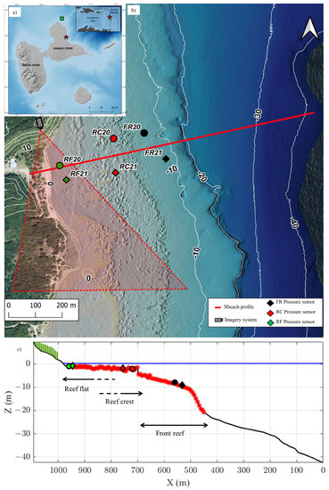
Figure 1.
(a) Anse-Maurice beach location map (b) Map with sensor locations (red, black or green markers), profile line (red line), camera location (grey rectangle), and camera field of view (red area). Beach and nearshore profile (c) showing the reef and upperbeach vegetation areas as well as the location of field measurements with pressure transducers.
3. The Numerical Model
3.1. Model Description
Xbeach is an open source numerical model developed to simulate nearshore processes, including hydrodynamics and morphodynamics [41]. So far, it has been successfully used in numerous environments, mainly sandy and gravel coasts but also in shores with vegetation [42] and reef-lined beaches e.g., [11,18,20,28,43]. In this study, the fully resolving mode called “non-hydrostatic” was used; hereafter this mode is referred to as XB-NH. It can resolve wave motions for very low frequency waves (VLF, wave frequency < 0.004 Hz), infragravity waves (IG, 0.004 < wave frequency > 0.04 Hz), short waves (SW, typical wave frequency > 0.04 Hz) and depth-averaged flow using non-linear shallow water equations with a non-hydrostatic pressure correction term [44]. This XB-NH mode was selected as it gives the best prediction of extreme runup events [20]. The model may also be used on a 2D horizontal grid or a 1D grid. The latter option was selected to reduce the computational cost, based on the number of simulations that was required for this investigation. Xbeach also has a morphology module that can assess the erosion associated with storm conditions; but this option was not used in this study. When using XB-NH, several parameters may be used to calibrate the model; particularly in the presence of coastal ecosystems. The coral reef is often represented using a suitable friction coefficient (), which represents the rugosity (or complexity) of the sea bottom that is not well-resolved by the bottom layer. This mimics the obstruction to the flow provided by the ecosystem’s features that are smaller than the model grid size, such as the coral colonies. Thus, the value applied to coral reefs is generally greater by about an order of magnitude when compared to a sandy surface. The value may be chosen by relying on previous research, by applying values that correspond to the morphologic area (e.g., reef slope and flat), by the nature of the bottom (e.g., sand and coral) or even by coral living percentages [11,28,45]. Empirical parameterization using a range of possible values and comparing against field measurements may also be used [20,46]. In this study, the commonly used value for sand (i.e., 0.001) is applied to areas where coral is absent (i.e., along the black line segment on the profile in Figure 1c). An empirical parameterization for coral areas is then undertaken to find a single value that best represents the local hydrodynamics (see Section 3.2). A typical range from the literature was applied and the best-fit value, when compared with the data, was selected for further analysis. For the vegetation, an additional layer on top of the bottom layer may be added. The vegetation is schematized as rigid horizontal cylinders as in most models e.g., [42,47,48]. The length of the cylinders (), their diameter (), their density (N) and their associated drag coefficient () are customizable. However, the effect of vegetation flexibility on the flow is not accounted for in this approach. The parameter is more suitable for use during calibration as all other parameters correspond to physical plant properties that may be directly measured on site.
3.2. Model Calibration
A representative profile of the study area was extracted for the modeling experiment (Figure 1c) from a Lidar dataset [49]. The coral reef and upperbeach vegetation parameterizations were calibrated using offshore conditions and on-site measurements. Offshore wave conditions were extracted from the spectral wave model (WW3) simulations provided through the MARC platform (https://marc.ifremer.fr/, accessed date: 13 March 2023) by the IFREMER. Sea-level conditions were extracted from the tide gauge located at Pointe à Pitre (https://data.shom.fr/, accessed date: 13 March 2023). Local storm conditions were extracted from the MARC model dataset, considering storm events occurred when the significant wave height, , exceeds 2.3 m. An of 2.3 m represents the 95th percentile wave height based on the time window of the camera observation period (i.e., 1045 days) which started on 14 April 2019 and ended on February 2nd 2022. Six (6) events (two (2) of which were above the storm threshold of 2.3 m and four (4) additional events which were slightly less energetic events) were extracted for the field measurement periods. A further sixteen (16) events were selected for the entire camera observation period, thus making a total of twenty-two (22) events. Waves and sea-level conditions, at the peak event, were used to force the XB-NH model. Table 1 summarizes hydrodynamics at the peaks of all 22 events, where events 1 to 6 correspond to the field measurement periods. Other than , Table 1 shows the peak wave period, , the peak wave direction, , and the daily maximum in TWL, dTWL.

Table 1.
Hydrodynamic inputs used for XB-NH model validation. It comprises peak conditions for the still water level (0), the significant wave height (), the peak wave period (), the peak wave direction () and the daily maximum still water level (dTWL).
For all events, the maximum TWLs modelled were compared to the TWL extracted from the camera. Additionally, events extracted during the wave measurement periods (event 1 to 6) were used for further calibration. Indeed, the SW, IG, and VLF bands and (wave setup) between the model and the on-site measurements were compared at each sensor position (i.e., FR, RC, and RF). is the increase in mean water level due to wave-driven mass transport on the reef flat. It is caused by wave breaking and radiation stresses. As the value is critical for interpretation of the results and to validate the most relevant coral parameter based on the literature review, a specialized calibration test was completed. On sandy areas, was assigned a fixed value of 0.001 according to [11]. For the coral reef area, a range between 0.001 and 0.15, with increments of 0.01, was assessed. Each parameterization was modelled for each of the storm conditions identified in Table 1. A comparison was made between the modelled and the measured wave heights at the different reef locations and for different wave frequency bands for events 1 to 6. The modelled TWL results were then compared with the video-derived TWL for events 7 to 22, and the free surface measurement on the RF for events 1 to 6. The TWL from the camera was extracted on a profile without vegetation to avoid potential interactions between ecosystems. The mean error between the measured and the simulated TWL value was calculated for all events for all simulations (Figure 2). The global TWL was affected by the magnitude of the friction coefficient (Figure 2k). The IG (Figure 2e,h) and VLF (Figure 2h,i) waves on the reef crest and reef flat were also affected by the parameter. On the opposite, SW presented a mild change with friction increasing (Figure 2b,c). There was also an insignificant influence of the parameter on the observed (Figure 2j). A value of 0.09 was selected as it coincides with the lowest mean error for the TWL and shows only small errors with the hydrodynamic parameters, especially on the reef flat.
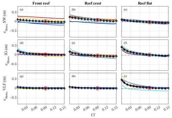
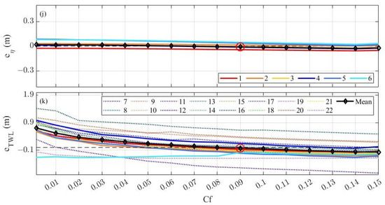
Figure 2.
Measured versus predicted hydrodynamic parameters and TWL depending on the bottom friction coefficient (). Error between measured Hrms/modelled Hrms, (a,d,g) on the front reef position, (b,e,h) on the reef crest position, and (c,f,i) on the reef flat and (a–c) for SW band (eHrmsSW), (d–f) for IG band (eHrmsIG), and (g–i) for VLF band (eHrmsVLF). (j) Measured/modelled wave-setup () in the reef flat. (k) Camera-derived total water level (TWL) against modelled TWL. On graphs (a–j) only the 6 events extracted from field measurements are plotted. On graph (k) the 16 storms extracted from the whole camera dataset are also plotted. The bold black line with diamonds represents the mean error on all storms for each value modelled. The red circle on each plot indicates the value (0.09) chosen after calibration.
For calibrating the vegetation cover parameterization, only the events exceeding the vegetation limit (event 8, 11, 12, 18, 19 and 21) were used (Table 1). Thus, for those events, a vegetation layer was added to the modelled profile and compared with the camera-derived TWL. In Xbeach, four vegetation characteristics can be adjusted (see Section 3.1). As Ipomoea pes-caprea represents the vast majority of the front layer of vegetation, the calibration was focused on this type of vegetation cover. Such vegetation is mainly crawling with horizontal stems and the schematization of vegetation as vertical cylinders in Xbeach is not directly suitable. Thus, the values of ah, bv and N were assigned using both on site observations and the literature [50] with values respectively of 0.3 m, 0.02 m, and 30 number of stem by meter. Additionally, the leaves of Ipomoea are particularly wide, which may impact the flow but this was not accounted for in the model. Nonetheless, the parameters associated to the vegetation observed on site were retained and the calibration of the coefficient was used to match as close as possible with the observations. Simulations were first completed with values ranging from 0.01 to 3, in increments of 0.5. These increments were reduced around values with the lowest error and a value of 1.25 was finally selected (Figure 3) for the next simulations. This numerical experiment on a range of values illustrates that the parameter has little impact on the TWL.
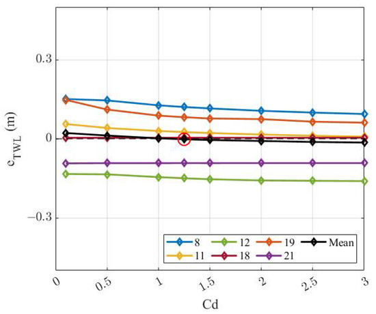
Figure 3.
Total water level (TWL) error for the event exceeding the vegetation, and the mean error for each drag coefficient () coefficient value modelled.
3.3. Model Strategy and Scenarios
3.3.1. Offshore Forcing
Once the model parameterization was calibrated based on observed events, a set of synthetic offshore hydrodynamic forcings was simulated. Hydrodynamic parameters include the still water level, 0, and offshore waves parameters (e.g., and ). To establish a range for the 0, a storm surge range was added to the calm condition sea-level range. The calm condition sea-level range was developed using the Pointe-à-Pitre tide-gauge and values ranged from −0.3 m to 0.5 m, in increments of 0.2 m, in the local altimetric system. The maximum value of the storm surge range was defined using the 100-year return period storm surge [38] at the offshore point of the model profile. Thus, a range from 0 m (no storm surge) to 1 m, with sampling intervals of 0.2 m, was used. The global 0 thus had a range from −0.3 m to 1.5 m with sampling intervals of 0.2 m. For wave forcings, the 100-year return period was also used as the maximum boundary and common wave condition for the minimum boundary. Thus, had a range from 2 m to 12 m, and a range from 6 secs to 18 secs was applied. By combining the 0, , and ranges, a set of 1463 unique hydrodynamic conditions were created with all the various combinations. Unlikely combinations of and were filtered using wave steepness, where is the offshore significant wave height and the offshore wave length, defined as the following:
where g represents the gravity in m/s. and pairs with an value lower than 0.005 or higher than 0.05 were rejected [10,21]. After filtering in this way, 1007 hydrodynamic scenarios remained. Each hydrodynamic condition was simulated on a 1024-s burst (17 min) which corresponds to the burst duration of the pressure sensors used in the validation. Additionally, the simulations were repeated with an addition of 0.82 m of 0 to account for sea-level rise in Guadeloupe Island. This 0.82 m magnitude corresponds to the IPCC (Intergovernmental Panel on Climate Change) RCP 8.5 scenario of SLR by 2100 in Guadeloupe [51]. This quite pessimistic scenario which corresponds to continued increase of greenhouse gas emissions, was selected to better assess the critical potential future changes in coastal inundation that could occur at reef-lined beaches.
3.3.2. Ecosystem Status
To depict differing states of the coral reef and upperbeach vegetation, three parameterizations were chosen corresponding to variable states: (1) reference ecosystem state derived from observations, (2) a deteriorated state, and (3) an enhanced state. For the coral reef, two parameters were used: the bottom friction and the depth over the reef (bottom layer elevation). Both parameters influenced the wave attenuation by the reef. The specific influence of is visible through the validation (Figure 2k) as increasing values of the coefficient gradually increase friction effect and so reduce the TWL. The effect of the water depth over the reef may be roughly assessed by looking at the impact of the storm used for the validation (Table 1). Indeed, events 1, 2, 3 or 18 for example, present similar incident wave conditions and 0 of 0.18 m or above. These conditions generated TWL of around 0.8 m while more energetic events 14, 15 and 16 but with 0 ranging between −0.2 m and −0.03 m only generated a TWL ranging from 0.12 m and 0.5 m. For the reference ecosystem state, the results from the validation were used with a value of 0.09 and the bottom layer extracted from the lidar. For the degraded state, a value of 0.05 was applied and 0.2 m water depth was added at the position of the reef. The objective of this was to imitate a further smoothening of the reef in case of further death of coral colonies as well as a destruction of skeletons. At the opposite, for the enhanced state, a value of 0.13 was applied as well as a decrease of 0.2 m in water depth. Here, the objective was to mimic a reef development up to a healthy state with highly developed living coral colonies. values for the degraded and enhanced states were chosen to be equally spaced from the reference ecosystem state (i.e., 0.09) and to be coherent with values from other sites in the literature [27,28,30]. Regarding the bottom changes, even though some coral species may reach growth rates exceeding 0.1 m/yr (e.g., Acropora) [52,53,54] a quite moderate change in bottom elevation was applied to match with a net coral development over nearly a decade. For the degraded state, an equally opposite change was applied to match the potential erosion of reference structures over approximately a decade. To support this assumption, one can refer to [55] who used the seafloor evolution over several decades and estimated the mean seafloor loss in coral reef ecosystems to be between −0.015 m/yr and 0.063 m/yr on 5 sites; 4 of which were in the Caribbean.
For the vegetation, the height (), the density (N) and the drag coefficient () were used to model the changes. The , N and parameters were adjusted for the various vegetation states assessed. The parameter had only a minimal effect on the TWL modulation as highlighted in the calibration procedure (Figure 3). For the reference ecosystem state, the results from the validation were used where = 0.3 m, = 0.02 m, N = 30 and = 1.25. For the enhanced status configuration, a density of 2 times the reference value (i.e., N = 60) was assumed, an additional 0.1 m in vegetation height was projected (i.e., = 0.4 m) which corresponds roughly to most developed patches on the site located inside the enclosures, and the drag coefficient was also enhanced to a = 2. This increased value aims to represent an increase in vegetation complexity and density. For the degraded scenario, the vegetation was simply removed. It represents a configuration where human trampling has resulted in the complete destruction of the vegetation. In fact, upperbeach vegetation is already absent at many cross-shore locations at the study site. Figure 4 schematizes the overall modeling experiment.
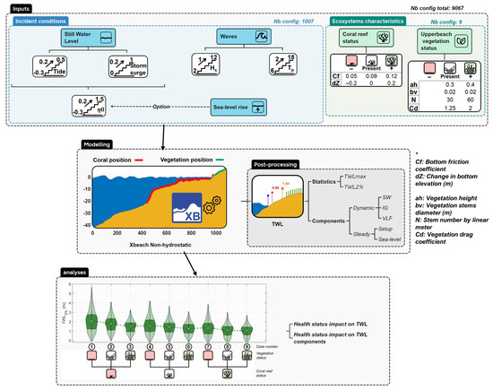
Figure 4.
Global modeling strategy flowchart. The incident conditions are detailed in the blue box which include ranges for the still water level (), the significan wave height () and pek period (). Ecosystems characteristics are detailed in the the green box. It includes the bottom friction coefficient () and the bottom layer change () for the coral reef and height (), stems diameter (), number of stems per linear meter (N) and drag coefficient () for the vegetation. The middle box schematizes modeling profile and output extractions. The lower box schematizes analyses performed on model outputs.
3.3.3. Post-Processing Modeling Outputs
Nine ecosystem configurations were modelled in this numerical experiment, and by combining these with the 1007 set of hydrodynamic conditions, resulted in 9063 configurations in total. The TWL components fall into two categories, steady components and dynamic components. The steady component is comprised of 0 and , and the dynamic component is the swash which may be disaggregated considering: (i) short saves (SW) associated with frequencies higher than 0.04 Hz, (ii) infragravity-waves (IG) associated with the frequencies between 0.004 and 0.04 Hz and (iii) very-low-frequency waves (VLF), associated with frequencies lower than 0.004 [56,57,58]. The TWL spectra at the shoreline level was extracted for each burst, and the 2% exceedance was computed for the total TWL (TWL2%) and for each frequency band (SW2%, IG2%, and VLF2%) [10,20]. Parameters were finally compiled and compared according to the associated ecosystem combination. In order to highlight the effect of ecosystem changes on the TWL2%, outputs from each ecosystem scenario were compared to the reference case (based on the current state). Average and maximum values of TWL2% were compared as well as the whole distribution of TWL2%. For the latter analysis with the entire distribution, quantiles were used. Thus, each TWL2% distribution data was subdivided in 100 equal parts so that the p-th quantile is the value greater than p % of the other values. Each quantile was then compared to its equivalent in the reference case.
4. Results
4.1. Impact of Ecosystems Status on TWL2%
Firstly, the distribution of the output variable (TWL2%) in relation to the forcing variables (, , and 0) was examined. As an example, Figure 5 represents the results of all hydrodynamic combinations (i.e., the 1007 scenarios) for the reference ecosystem configuration state (identified as case 5). The most extreme flooding events (TWL2% near to 3.5 m), are associated with the most intense waves and higher values of 0. Figure 5b represents the structure of the modeling experiment; it shows all the hydrodynamic scenarios where several random pathways are highlighted in black for illustration. Figure 5a gives a different visualization of the input hydrodynamic conditions and the associated output TWL2%. To estimate the respective influence of the incident variables on the TWL2%, we calculated the linear correlations for all ecosystem configurations. TWL2% appears to be firstly controlled by 0 (on average R2 = 0.74 over all ecosystem configurations), then (on average R2 = 0.61) and lastly (on average R2 = 0.40).
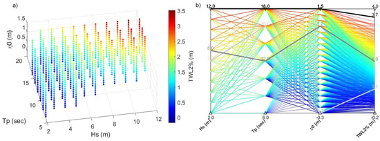
Figure 5.
Entire set of modeling scenarios (triplet , , 0) and results for reference coral reef and upperbeach vegetation configuration. Three-dimensional scatter (a) and parallel (b) plots with input variables , , and 0, and output variable TWL2%. The color scale is the same on both graphs. Four random paths on (b) are highlighted (black lines).
The entire distribution of TWL2% was calculated to highlight the control of ecosystem status on the TWL2% (Figure 6). For each configuration, the white point indicates to the average TWL2% for all hydrodynamic conditions. The reference ecosystem configuration (case 5) shows a peak at 3.5 m and an average value of TWL2% of 1.6 m. The configuration with both ecosystems in degraded status (case 1) presented the highest TWL2% values with peaks reaching near 6 m (i.e., +47.3% in average compared to reference configuration) and the configuration with both ecosystems in better status (case 9) had the lowest values with a maximum at 2.75 m (i.e., −28.6% in mean compared to reference configuration). Assuming constant coral reef status, the configuration with the degraded vegetation shows higher TWL2% peak values (e.g., case 4). Assuming a constant vegetation status, the coral reef status affects the whole TWL2% distribution (e.g., case 2). This assessment is verified in Figure 7 which represents the difference in quantiles for each ecosystem configuration against the reference case. From this figure, we see that when the vegetation status is changed, the difference between the reference case increases with the higher quantiles. It means that for low values of TWL2%, the difference with the reference ecosystem is low while for high values of TWL2%, the difference is important. In other words, the vegetation effect is particularly efficient for the highest TWL2%. This is simply because the vegetation limit is not reached for every condition. Thus, the vegetation may affect the TWL2% only when it is reached, typically for the highest incident conditions. Just to note for the reference case (case 5), of the 1007 hydrodynamic conditions, 879 (87%) actually reached the vegetation limit. By looking at the configurations where only the reef status changes (cases 2 and 8), we observe the same mechanism but to a lesser extent. Certainly, the difference is already significant for the lowest values of the TWL2% quantiles but slightly increases for higher values. Furthermore, it is noted that the combination of a degraded and an enhanced ecosystem has a beneficial effect on the resulting TWL2% (cases 3 and 7). The configuration of a degraded coral reef and vegetation in enhanced status (case 3) led to TWL2% very close to the reference and even a reduction for highest quantiles. The opposite configuration (case 7) presented even better results with a slightly improved attenuation for every quantile except the most extremes ones. Lastly, these results suggest that the loss of both ecosystems (case 1) would potentially increase TWL2%, approaching 2 m for upper quantiles, while an improvement in both ecosystem statuses (case 9) would lead to a decrease, approaching 1 m.
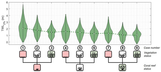
Figure 6.
TWL distribution for each ecosystem configuration. The means are represented by a white point and portions between the first (0.25) and third (0.75) quartiles in the darker green color. Each ecosystem configuration is presented as pictograms to represent the status of the ecosystem (the red pictograms are for the degraded ecosystem state, the white for reference or current ecosystem state and the green for the enhanced ecosystem state).
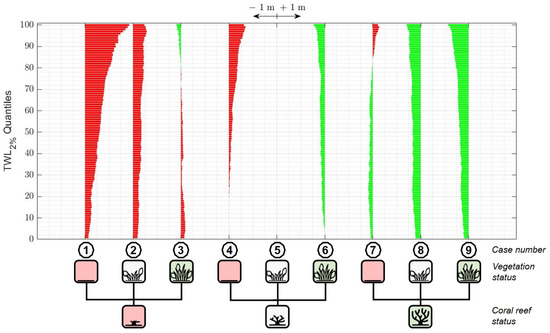
Figure 7.
TWL2% differences against reference configuration expressed with quantiles. Values greater than reference are represented in red and values lower than reference in green. Each ecosystem configuration is presented, pictograms represent the status of the ecosystem. The arrows give the scale of a difference of one meter on the X axis.
To further examine the evolution of the TWL2% differences with the reference case, we analyzed its variations with the incident conditions (Figure 8). We chose to focus this analysis on 0 and as is weakly correlated to the TWL2%. This assessment provides further information on the impact of ecosystem status on the TWL components. The evolution of TWL2% with coral reef status appears poorly related to the 0 but well correlated with the (e.g., Figure 8: cases 2, 5 and 8). For the most extreme , and against the reference case, a TWL reduction exceeding 0.5 m was observed for the enhanced reef (case 8) and a TWL2% increase exceeding 0.5 m was obtained for the degraded reef (case 2). The evolution of TWL2% with the vegetation status is correlated with both 0 and (e.g., Figure 8: cases 4, 5 and 6). Thus, for the strongest incident conditions, and against the reference case, a TWL2% decrease of up to 0.25 m was observed for case 8, and an increase of up to 0.5 m for case 4. Mixed ecosystem configurations induced a particular TWL2% response. Indeed, the case 3 configuration provides a TWL2% amplification for the lowest values of incident 0 conditions up to mid-range and an attenuation for the second portion of the 0 range. Whereas the case 7 configuration presents an attenuation of TWL2% for 0 up 0.5 m but an increase in TWL2% above this threshold. This processing verifies observations made in Figure 7 and adds new elements to the understanding of the influence of and 0 on TWL2%.
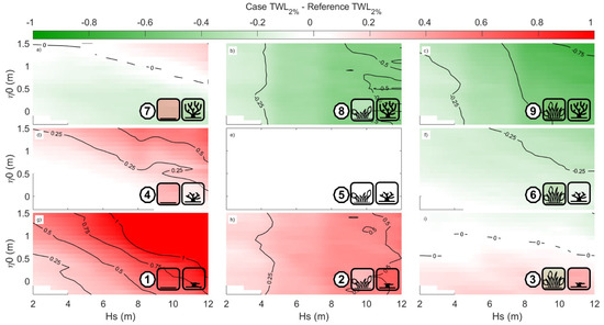
Figure 8.
Difference in TWL2% relative to the reference case as a function of 0 and , the differential color is then expressed in meters. Pictograms represent the status of the ecosystem. On the figures (a–i), coral reef status changes from bottom to top, and the vegetation status from left to right.
4.2. Influence of Ecosystems Status on TWL2% Components
For all simulations, the different components that are involved in generating the TWL2% are separated in order to evaluate their relative contribution (Figure 9). For the steady components (Figure 9a), the 0 is constant over all configurations as it is an input parameter; it corresponds to an offshore TWL which applies regardless the ecosystem. The varies weakly and seems mainly correlated with coral reef status only. For the dynamic components (Figure 9b), the IG waves dominate for all configurations with a net attenuation depending on coral reef status. VLF waves follow the same behavior as the IG waves. However, the SW band is influenced by both the vegetation’s and the coral reef’s statuses. Consequently, from the worst-case scenario (case 1) to the best-case scenario (case 9), the mean relative contribution of the dynamic component decreases comparatively to the steady components (Figure 9c). Thus, on all configurations with an enhanced reef (cases 7, 8 and 9) and on configurations with the reference reef and enhanced or reference vegetation (cases 5 and 6), the steady component dominates in average values and extremes. On configurations with reference reef and degraded vegetation (case 4) as well as with degraded reef and enhanced or reference vegetation (case 3), both components are close on average and for extremes. In the worst-case scenario (case 1), the dynamic component is clearly dominant on average and for extremes.
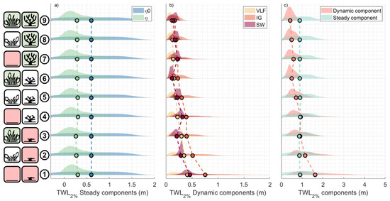
Figure 9.
(a) Steady components ( and 0) of the TWL2%, (b) Dynamic components (SW, IG and VLF) of the TWL2%, (c) Global dynamic and steady components of the TWL2%. The dots represent the mean for each variable and ecosystem status. The shaded areas represent the distribution for each variable. Each ecosystem configuration is represented, and ecosystem status is indicated by the pictograms on the left.
5. Discussion
5.1. Coral Reef and Upperbeach Vegetation Impact on Coastal Flooding
In this study, a quantitative assessment of the effect of different states of coral reef and upperbeach vegetation on TWL was provided where the various states reflect the different structural composition of the ecosystems. Although the schematization remains simplified, the combination of the two ecosystems in numerical modeling is innovative and provides new elements on the understanding of the physical processes. The depiction of the bottom complexity, through directly applying a value of the associated frictional coefficient for modeling, still constitutes a scientific challenge. In this study, an empirical approach based on existing literature was used to determine the relevant coefficients (i.e., for the coral reef and for the vegetation). Scenarios with the different ecosystem’s statuses are understandably theoretical. However, they strive to reproduce realistic changes that have happened in the past and may happen in the future, on a decadal timescale. These scenarios were based on existing literature [27,28,30,52,53,54,55] and the empirical observations of the characteristics of the coral reef and vegetation observed on site. With such parameterizations, results clearly indicate the importance of the ecosystem’s status on the resulting TWL2%. A change in the ecosystem status has limited influence on the steady components of the TWL2%, even though is slightly lower for degraded reef scenarios. This statement was already made by [43] who argued that the reduction of bottom friction has limited effect on . It is here hypothetized that the lowered observed setup is principally a consequence of the change in bottom elevation () and the wave breaking resulting from that change. Conversely, the dynamic (wave-induced) components present a clear response to ecosystem changes with lesser intensity on enhanced ecosystem configurations and higher intensity on degraded ecosystem configurations. Consequently, the proportion of the dynamic components is greater for degraded scenarios than for enhanced scenarios. Additionally, the two ecosystems have a variable influence on the TWL. A change in the coral reef structural status affects the overall distribution of TWL2% (cases 2 and 8 on Figure 6 and Figure 7) an observation which was also made by [30], and our results show a slightly larger influence on the most intense TWL2%. However, a change in the vegetation status only affects the most intense TWL2% (cases 4 and 6 on Figure 6 and Figure 7). The loss (case 2 on Figure 8) or gain (case 8 on Figure 8) in the coral structure influences the TWL2% such that it increases almost linearly with . This signifies that the wave attenuation by the reef is particularly efficient for strong waves. These results differ from those of [29] where the loss of reef impacted the runup for storms with return periods of one to five years, while almost no change was noted for the most extreme storms. We hypothetize that the difference from the previous study is the result of the choice in reef state change parameterization. In their study [29], coral degradation scenarios were created by reducing the elevation of the bottom layer to specifically evaluate the influence of this reef state parameter. However, in our experiment both the bottom elevation and rugosity are varied. In the current study, the coral status particularly impacts the low frequency components of the TWL2%. Indeed, for case 2 (i.e., the degraded reef status) led to significant augmentation of the mean and maximum IG and VLF contribution (+40% mean IG contribution), while for case 7 (i.e., the enhanced reef status) reduced IG and VLF contribution (−25% mean IG contribution). However, the SW contribution did not vary significantly. Moreover, as was highlighted by the coefficient calibration, the bottom friction mainly affects low-frequency waves. This observation of an increasing IG contribution with reduction of reef smoothness had also been highlighted by another study [59,60]. Furthermore, in a metamodel experiment, [10] demonstrated that 0 is correlated with the IG wave band. The degraded coral reef cases (cases 1, 2 and 3) have a low value which is associated with a greater water depth over the reef and suggests an augmented contribution of low frequency waves for these scenarios. Therefore, it is crucial to evaluate the potential changes in reef elevation and roughness when assessing the impact of coral reef state on TWL, as these results highlight their significance. Overall, the destruction of current coral structures would lead to further dominance of low frequency waves in generating the highest TWL.
Previous research has extensively investigated the impact of various vegetation ecosystems, such as mangroves, seagrasses, salt marshes, and dune vegetation, on coastal hazards. However, the effects of tropical upperbeach vegetation have received little attention [50,61]. This study aims to address this gap by quantifying the role of upperbeach vegetation in reducing total water level (TWL) and highlights the importance of preserving or restoring this vegetation in reef-fronted beaches. Specifically, this research emphasizes the crucial role played by upperbeach vegetation in limiting the extent of swash inland, thereby reducing the risk of flooding. It was noted that the vegetation was reached for 879 hydrodynamic conditions of the 1007 scenarios of the reference case (case 5), which means that the vegetation does not interact with incident conditions of mild intensity. When the vegetation is effectively crossed, the dampening of the flow is correlated with the distance of vegetation crossed by the flow. As evidenced in Figure 6, Figure 7 and Figure 8 (cases 4, 5 and 6), vegetation mainly affects extreme values of TWL2% (associated with the highest incidents eta0 and ). These more energetic conditions lead to further propagation of the swash inland and so result in an increasing interaction with the upper beach vegetation. The importance of the vegetation width on the attenuation has also been highlighted for other vegetation types like mangroves and seagrasses [2,62]. Even though vegetation status demonstrated a significant effect on all frequency bands, it induced a greater response in the SW band, showing a mean change of around +/− 45%.
Finally, the literature has not extensively explored the impact of combined ecosystems on nearshore hydrodynamics [29,30] particularly in the case of coral reefs and upper beach vegetation, a configuration commonly found on tropical shores. In this study, this study sheds light on the specific response of TWL2% to various combinations of upper beach vegetation and coral reefs in different statuses. Combining an enhanced reef with a degraded vegetation (case 7) led to an attenuation of TWL2% for low and moderate offshore conditions, and a slight increase for the most extreme wave and 0 conditions. Combining a degraded reef and healthier vegetation (case 3) yields the opposite, where the attenuation by the vegetation becomes more efficient when the 0 exceeds 1 m, regardless of the offshore (Figure 8i). In such a situation, the vegetation width that is crossed by the swash is expected to be larger, enhancing the attenuation effect.
5.2. Expectations for Changes in Coastal Flooding in the Future
This numerical experiment included the investigation of a RCP8.5 SLR scenario for 2100 as hydrodynamic input and assessed the future impact of different ecosystems’ health status in coastal inundation (Figure 10). The SLR scenario adds an additional elevation of 0.82 m to the 0 for each hydrodynamic condition. Even though the TWL2% increased for all ecosystem configurations under this sea-level rise scenario, the increase differed among ecosystem configurations. On the reference scenario, the average TWL2% increased by 0.8 m and the maximum TWL2% increased by 0.35 m. For the cases with different reef statuses (refer to cases 2, 5 and 8), the augmentation compared to present day simulations is particularly important for the enhanced reef configuration (case 8). Since wave filtering by the reef is depth-dependent [10,11,12], this drastic depth addition decreased the reef’s ability to dampen the waves. With the RCP8.5 SLR scenario for 2100, the TWL2% associated with the enhanced reef almost reached the reference scenario TWL2% levels. This indicates that, in the future, the wave transformation by the reef will decrease over time regardless of the state of the reef. The only way to maintain a constant level of protection would be to have a coral growth able to keep up with the rate of sea-level rise. Studies have proved that some healthy reefs may achieve that [63,64] but the current dynamics of most Caribbean reefs is not sufficient to support this “keep-up” growth [65]. The enhanced case here acts as a moderate adaptation to the SLR with realistic coral reef growth rate. [9] identified the reef complexity as the main control on wave energy dissipation on future reefs under SLR. Here, we saw that even our best case scenario of coral reef state (case 8) under SLR is not enough to sustain the same level of protection compared to the present day reference (case5).
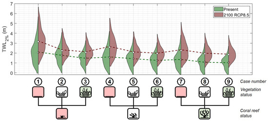
Figure 10.
TWL distribution for each ecosystem configuration for present day and sea-level scenario RCP8.5 for 2100.
It was observed that the degraded vegetation status shows great differences in comparison to their present-day equivalent. As the reef protection is reduced for the SLR scenarios, the remaining energy reaching the shoreline level is more important, and the role of the vegetation in TWL2% attenuation is greater as the vegetation is reached more frequently. Thus, its disappearance leads to a drastic increase in TWL2%. For this modelling experiment the vegetation is simplified to a fixed simple vegetation layer. The erosion of the vegetation layer that may occur during storms is not accounted for, which could overestimate the role of the vegetation during storm events. However, to provide a more realistic case, the vegetation position has been moved back compared to present-day simulations to a position that accounts for the SLR (+0.82 m). The vegetation that develops at this position is of a different type and increased complexity. It comprises a crawling layer, but also includes shrubs and trees. This combination of vegetation is more prone to resist storm erosion and would provide a greater obstruction to swash propagation. Our results indicate that the vegetation could partially compensate for the loss of coral reef, which is crucial information in a context of global coral disappearance. In addition, the experiment using the RCP8.5 SLR scenario revealed a loss in coral reef wave attenuation even for the enhanced reef configuration.
5.3. Planning Recommendations
Significant evidence states that coral reefs will suffer from the effects of climate change and in particular sea temperature rise, which will trigger more frequent bleaching events. Caribbean reefs have been suffering for a few decades and are declining all over the region [66,67]. If this trend continues, the nearshores of reef-lined beaches are expected to become smoother and deeper over time. Our results indicate that, in the case of coral reef degradation, the loss of the coral reef attenuation impact on waves and the TWL may be partially compensated for by upperbeach vegetation, assuming the vegetation retains its capacity to resist extreme events and mitigate against coastal flooding. Actions to establish new corals or restore coral reef health are expensive and may be fated to fail if the main drivers affecting the reef are global in nature. Restoring vegetation is easier, cheaper and much quicker in achieving effectiveness than restoring coral reefs [68,69]. In addition, even though the vegetation may be affected by storms, the natural recovery process is usually quicker than for corals; in particular, in the tropical context where crawling vegetation growth can be observed in a very short time (days to weeks). In any case, direct actions may be engaged to quickly restore the vegetation to regain a pre-storm state. Given the results of this study, a recommendation can be made to encourage the restoration and maintenance of a complex and dense upperbeach vegetation layer that may provide a low cost and efficient compromise to protect the coast from large storm flooding events in the future. Obviously, actions to maintain and restore coral reefs are supplementary, and should also be increased to optimize the coastal protection and benefits from the other services provided by this ecosystem.
6. Conclusions
This study reports the response of coastal flooding (expressed through the TWL2%) to different combinations of coral reef and upperbeach statuses. By utilizing the XB-NH model on a cross-shore profile, the hydrodynamic conditions for a return period of 100 years were simulated. Firslty, the findings confirm observations that have been previously made in the literature, namely that:
- Ecosystem degradation results in an increase in the TWL.
- Coral reef degradation leads to an increase in low-frequency motions in the nearshore area.
- The impact of the vegetation on the swash is dependent on the distance crossed by the flow.
The study also provides new elements on comprehension of the processes involved in ecosystem combinations, which are:
- Combining a degraded coral reef and a healthier upperbeach vegetation induced an increase of TWL2% for low and moderate offshore conditions but an attenuation for the most extreme offshore conditions. So upperbeach vegetation could compensate for losses in the coral reef for the most extreme conditions.
- With both ecosystems having a healthier status, a reduced TWL by up to 0.7 m (25%).
- Further degradation of both ecosystems can lead to an increase in the TWL that can exceed 1 m can result.
Finally, in the future, where a sea-level rise is anticipated, it is expected that:
- The sea-level rise will likely exceed the reef’s capacity to grow, as reefs will deepen and progressively lose their effect on wave attenuation even though they may have a high structural complexity.
- With the loss of reef protection, the relative effect of the upperbeach vegetation will increase assuming beach morphological adaptation occurs, that the vegetation retains its ability to resist the most extreme waves and the vegetation is able to recover rapidly.
These findings are crucial for coastal management strategies and nature-based solutions in similar reef-lined beaches and should encourage active protection and development of upperbeach vegetation density and complexity.
Author Contributions
Conceptualization, T.L., Y.B. and D.V.-L.; methodology, T.L., A.N.L. and N.V.; software, T.L. and N.V.; validation, T.L.; formal analysis, T.L. and Y.B.; investigation, T.L. and M.M.; writing—original draft preparation, T.L.; writing—review and editing, T.L., Y.B., D.V.-L., A.N.L., N.V., M.M. and Y.D.L.T.; visualization, T.L.; supervision, T.L., Y.B., D.V.-L. and Y.D.L.T. project admin-istration, Y.B. and Y.D.L.T.; funding acquisition, Y.B. and Y.D.L.T. All authors have read and agreed to the published version of the manuscript.
Funding
This research was funded by the EU INTEREG Caribbean CARIB-COAST project (grant number 4907).
Institutional Review Board Statement
Not applicable.
Informed Consent Statement
Not applicable.
Data Availability Statement
Data available on request.
Acknowledgments
The authors would like to thank Norden M., Delahaye T., Civallero E. and Chapron S. for their valuable help during the field experiments.
Conflicts of Interest
The authors declare no conflict of interest.
References
- Guannel, G.; Ruggiero, P.; Faries, J.; Arkema, K.; Pinsky, M.; Gelfenbaum, G.; Guerry, A.; Kim, C.K. Integrated modeling framework to quantify the coastal protection services supplied by vegetation. J. Geophys. Res. Ocean. 2015, 120, 324–345. [Google Scholar] [CrossRef]
- Infantes, E.; Orfila, A.; Simarro, G.; Terrados, J.; Luhar, M.; Nepf, H. Effect of a seagrass (Posidonia oceanica) meadow on wave propagation. Mar. Ecol. Prog. Ser. 2012, 456, 63–72. [Google Scholar] [CrossRef]
- James, R.; Lynch, A.; Herman, P.; Katwijk, M.; Tussenbroek, B.; Dijkstra, H.; Westen, R.; Boog, C.; Klees, R.; Pietrzak, J.; et al. Tropical Biogeomorphic Seagrass Landscapes for Coastal Protection: Persistence and Wave Attenuation During Major Storms Events. Ecosystems 2021, 24, 301–318. [Google Scholar] [CrossRef]
- Maza, M.; Lara, J.; Losada, I.; Ondiviela, B.; Trinogga, J.; Bouma, T. Large-scale 3-D experiments of wave and current interaction with real vegetation. Part 2: Experimental analysis. Coast. Eng. 2015, 106, 73–86. [Google Scholar] [CrossRef]
- Anderson, M.; Smith, J.; McKay, S. Wave Dissipation by Vegetation; US Army Corps of Engineers Engineer Research and Development Center: Vicksburg, MS, USA, 2011; p. 22. [Google Scholar]
- Miller, T.; Gornish, E.; Buckley, H. Climate and coastal dune vegetation: Disturbance, recovery, and succession. Plant Ecol. 2010, 206, 97–104. [Google Scholar] [CrossRef]
- Evelpidou, N.; Petropoulos, A.; Karkani, A.; Saitis, G. Evidence of Coastal Changes in the West Coast of Naxos Island, Cyclades, Greece. J. Mar. Sci. Eng. 2021, 9, 1427. [Google Scholar] [CrossRef]
- Ferrario, F.; Beck, M.; Storlazzi, C.; Micheli, F.; Shepard, C.; Airoldi, L. The effectiveness of coral reefs for coastal hazard risk reduction and adaptation. Nat. Commun. 2014, 5, 3794. [Google Scholar] [CrossRef]
- Harris, D.; Rovere, A.; Casella, E.; Power, H.; Canavesio, R.; Collin, A.; Pomeroy, A.; Webster, J.; Parravicini, V. Coral reef structural complexity provides important coastal protection from waves under rising sea levels. Sci. Adv. 2018, 4, eaao4350. [Google Scholar] [CrossRef]
- Pearson, S.; Storlazzi, C.; Dongeren, A.; Tissier, M.; Reniers, A. A Bayesian-Based System to Assess Wave-Driven Flooding Hazards on Coral Reef-Lined Coasts. J. Geophys. Res. Ocean. 2017, 122, 10099–10117. [Google Scholar] [CrossRef]
- Quataert, E.; Storlazzi, C.; van Rooijen, A.; Cheriton, O.; van Dongeren, A. The influence of coral reefs and climate change on wave-driven flooding of tropical coastlines. Geophys. Res. Lett. 2015, 42, 6407–6415. [Google Scholar] [CrossRef]
- Storlazzi, C.; Elias, E.; Field, M.; Presto, M. Numerical modeling of the impact of sea-level rise on fringing coral reef hydrodynamics and sediment transport. Coral Reefs 2011, 30, 83–96. [Google Scholar] [CrossRef]
- Storlazzi, C.; Gingerich, S.; Dongeren, A.; Cheriton, O.; Swarzenski, P.; Quataert, E.; Voss, C.; Field, D.; Annamalai, H.; Piniak, G.; et al. Most atolls will be uninhabitable by the mid-21st century because of sea-level rise exacerbating wave-driven flooding. Sci. Adv. 2018, 4, eaap9741. [Google Scholar] [CrossRef] [PubMed]
- Beetham, E.; Kench, P.; O’Callaghan, J.; Popinet, S. Wave transformation and shoreline water level on Funafuti Atoll, Tuvalu Edward. J. Geophys. Res. Ocean. 2016, 121, 6762–6778. [Google Scholar] [CrossRef]
- Roeber, V.; Bricker, J. Destructive tsunami-like wave generated by surf beat over a coral reef during Typhoon Haiyan. Nat. Commun. 2015, 6, 7854. [Google Scholar] [CrossRef] [PubMed]
- Dongeren, A.; Lowe, R.; Pomeroy, A.; Trang, D.; Roelvink, D.; Symonds, G.; Ranasinghe, R. Numerical modeling of low-frequency wave dynamics over a fringing coral reef. Coast. Eng. 2013, 73, 178–190. [Google Scholar] [CrossRef]
- Beetham, E.; Kench, P. Predicting wave overtopping thresholds on coral reef-island shorelines with future sea-level rise. Nat. Commun. 2018, 9, 3997. [Google Scholar] [CrossRef]
- Bruch, W.; Cordier, E.; Floc’h, F.; G, P.S. Water Level Modulation of Wave Transformation, Setup and Runup over La Saline Fringing Reef. J. Geophys. Res. Ocean. 2022, 127, e2022JC018570. [Google Scholar] [CrossRef]
- Lashley, C.; Roelvink, D.; Dongeren, A.; Buckley, M.; Lowe, R. Nonhydrostatic and surfbeat model predictions of extreme wave run-up in fringing reef environments. Coast. Eng. 2018, 137, 11–27. [Google Scholar] [CrossRef]
- Quataert, E.; Storlazzi, C.; Dongeren, A.; McCall, R. The importance of explicitly modelling sea-swell waves for runup on reef-lined coasts. Coast. Eng. 2020, 160, 103704. [Google Scholar] [CrossRef]
- Rueda, A.; Cagigal, L.; Pearson, S.; Antolínez, J.; Storlazzi, C.; Dongeren, A.; Camus, P.; Mendez, F. HyCReWW: A Hybrid Coral Reef Wave and Water level metamodel. Comput. Geosci. 2019, 127, 85–90. [Google Scholar] [CrossRef]
- Astorga-Moar, A.; Baldock, T. Assessment and optimisation of runup formulae for beaches fronted by fringing reefs based on physical experiments. Coast. Eng. 2022, 176, 104163. [Google Scholar] [CrossRef]
- Franklin, G.; Torres-Freyermuth, A. On the runup parameterisation for reef-lined coasts. Ocean. Model. 2022, 169, 101929. [Google Scholar] [CrossRef]
- Roelvink, F.; Storlazzi, C.; Dongeren, A.; Pearson, S. Coral Reef Restorations Can Be Optimized to Reduce Coastal Flooding Hazards. Front. Mar. Sci. 2021, 8, 653945. [Google Scholar] [CrossRef]
- Storlazzi, C.D.; Reguero, B.G.; Cumming, K.A.; Cole, A.D.; Shope, J.B. Rigorously Valuing the Potential Coastal Hazard Risk Reduction Provided by Coral Reef Restoration in Florida and Puerto Rico. In U.S. Geological Survey; 2021; pp. 1–24. Available online: https://pubs.usgs.gov/of/2021/1054/ofr20211054.pdf (accessed on 13 March 2023).
- Grady, A.; Moore, L.; Storlazzi, C.; Elias, E.; Reidenbach, M. The influence of sea level rise and changes in fringing reef morphology on gradients in alongshore sediment transport. Geophys. Res. Lett. 2013, 40, 3096–3101. [Google Scholar] [CrossRef]
- Reguero, B.; Secaira, F.; Toimil, A.; Escudero, M.; Díaz-Simal, P.; Beck, M.; Silva, R.; Storlazzi, C.; Losada, I. The risk reduction benefits of the mesoamerican reef in Mexico. Front. Earth Sci. 2019, 7, 125. [Google Scholar] [CrossRef]
- Storlazzi, C.; Reguero, B.; Cole, A.; Lowe, E.; Shope, J.; Gibbs, A.; Nickel, B.; McCall, R.; Dongeren, A.; Beck, M. Rigorously Valuing the Role of U.S. Coral Reefs in Coastal Hazard Risk Reduction. Usgs Open-File Report 2019-1027, 42. 2019. Available online: https://pubs.er.usgs.gov/publication/ofr20191027 (accessed on 13 March 2023).
- Franklin, G.L.; Torres-Freyermuth, A.; Medellin, G.; Allende-Arandia, M.E.; Appendini, C.M. The role of the reef-dune system in coastal protection in Puerto Morelos (Mexico). Nat. Hazards Earth Syst. Sci. 2018, 18, 1247–1260. [Google Scholar] [CrossRef]
- Guannel, G.; Arkema, K.; Ruggiero, P.; Verutes, G. The power of three: Coral reefs, seagrasses and mangroves protect coastal regions and increase their resilience. PLoS ONE 2016, 11, e0158094. [Google Scholar] [CrossRef] [PubMed]
- Ellison, J. Pacific Island Beaches: Values, Threats and Rehabilitation. In Beach Management Tools—Concepts, Methodologies and Case Studies; Botero, C., Cervantes, O., Finkl, C., Eds.; Springer International Publishing: Berlin/Heidelberg, Germany, 2018; pp. 679–700. [Google Scholar] [CrossRef]
- Johnston, E.; Ellison, J. Evaluation of beach rehabilitation success, Turners Beach, Tasmania. J. Coast. Conserv. 2014, 18, 617–629. [Google Scholar] [CrossRef]
- CEREMA. Fiches Synthétiques de Mesure des États de Mer—Tome 3—Outre-Mer. 2021. Available online: https://www.cerema.fr/fr/centre-ressources/boutique/fiches-synthetiques-mesure-etats-mer-maj-2021 (accessed on 13 March 2023).
- Reguero, B.; Méndez, F.; Losada, I. Variability of multivariate wave climate in Latin America and the Caribbean. Glob. Planet. Chang. 2013, 100, 70–84. [Google Scholar] [CrossRef]
- Service Hydrographique et Océanographique de la Marine. Références Altimétriques Maritimes—Édition 2020. Online, 2020. Available online: https://diffusion.shom.fr/donnees/references-verticales/references-altimetriques-maritimes-ram.html (accessed on 13 March 2023).
- Laigre, T.; Balouin, Y.; Nicolae-Lerma, A.; Moisan, M.; Valentini, N.; Villaroel-Lamb, D.; Torre, Y. Seasonal and episodic runup variability on a Caribbean reef-lined beach. Authorea 2022. [Google Scholar] [CrossRef]
- Torres, R.; Tsimplis, M. Seasonal sea level cycle in the Caribbean Sea. J. Geophys. Res. Ocean. 2012, 117, 1–18. [Google Scholar] [CrossRef]
- Krien, Y.; Dudon, B.; Roger, J.; Zahibo, N. Probabilistic hurricane-induced storm surge hazard assessment in Guadeloupe, Lesser Antilles. Nat. Hazards Earth Syst. Sci. 2015, 15, 1711–1720. [Google Scholar] [CrossRef]
- Valentini, N.; Balouin, Y. Assessment of a smartphone-based camera system for coastal image segmentation and Sargassum monitoring. J. Mar. Sci. Eng. 2020, 8, 23. [Google Scholar] [CrossRef]
- Moisan, M.; Delahaye, T.; Laigre, T.; Valentini, N. Suivi des Échouages de Sargasse et de l’Évolution du Trait de côte par Caméra Autonome en Guadeloupe: Analyse des RÉsultats et Bilan des Observations. Rapport Final. In BRGM/RP-712-FR; 2021; Available online: http://ficheinfoterre.brgm.fr/document/RP-71295-FR (accessed on 13 March 2023).
- Roelvink, D.; Reniers, A.; Dongeren, A.; Vries, J.; McCall, R.; Lescinski, J. Modelling storm impacts on beaches, dunes and barrier islands. Coast. Eng. 2009, 56, 1133–1152. [Google Scholar] [CrossRef]
- Rooijen, V.; Dongeren, V.; Version, D.; Research-oceans, J.; Rooijen, V.; Dongeren, V. Modeling the effect of wave-vegetation interaction on wave setup. J. Geophys. Res. Ocean. 2016, 121, 4341–4359. [Google Scholar] [CrossRef]
- Buckley, M.; Lowe, R.; Hansen, J.; Dongeren, A. Dynamics of wave setup over a steeply sloping fringing reef. J. Phys. Oceanogr. 2015, 45, 3005–3023. [Google Scholar] [CrossRef]
- Roelvink, D.; McCall, R.; Mehvar, S.; Nederhoff, K.; Dastgheib, A. Improving predictions of swash dynamics in XBeach: The role of groupiness and incident-band runup. Coast. Eng. 2018, 134, 103–123. [Google Scholar] [CrossRef]
- Péquignet, A.; Becker, J.; Merrifield, M.; Boc, S. The dissipation of wind wave energy across a fringing reef at Ipan. Guam. Coral Reefs 2011, 30, 71–82. [Google Scholar] [CrossRef]
- Risandi, J.; Rijnsdorp, D.; Hansen, J.; Lowe, R. Hydrodynamic modeling of a reef-fringed pocket beach using a phase-resolved non-hydrostatic model. J. Mar. Sci. Eng. 2020, 8, 877. [Google Scholar] [CrossRef]
- Suzuki, T.; Hu, Z.; Kumada, K.; Phan, L.; Zijlema, M. Non-hydrostatic modeling of drag, inertia and porous effects in wave propagation over dense vegetation fields. Coast. Eng. 2019, 149, 49–64. [Google Scholar] [CrossRef]
- Tang, J.; Shen, S.; Wang, H. Numerical model for coastal wave propagation through mild slope zone in the presence of rigid vegetation. Coast. Eng. 2015, 97, 53–59. [Google Scholar] [CrossRef]
- SHOM. LITTO3D® Guadeloupe. 2016. Available online: https://diffusion.shom.fr/donnees/altimetrie-littorale/litto3d-guad2016.html (accessed on 13 March 2023).
- Maximiliano-Cordova, C.; Salgado, K.; Martínez, M.; Mendoza, E.; Silva, R.; Guevara, R.; Feagin, R. Does the Functional Richness of Plants Reduce Wave Erosion on Embryo Coastal Dunes? Estuaries Coasts 2019, 42, 1730–1741. [Google Scholar] [CrossRef]
- Le Cozannet, G.; Idier, D.; Michele, M.; Legendre, Y.; Moisan, M.; Pedreros, R.; Rc, D. Timescales of emergence of chronic flooding in the major economic center of Guadeloupe. Nat. Hazards Earth Syst. Sci. 2021, 21, 703–722. [Google Scholar] [CrossRef]
- Buddemeier, R.; Smith, S. Coral reef growth in an era of rapidly rising sea level: Predictions and suggestions for long-term research. Coral Reefs 1988, 7, 51–56. [Google Scholar] [CrossRef]
- Lange, I.; Perry, C. A quick, easy and non-invasive method to quantify coral growth rates using photogrammetry and 3D model comparisons. Methods Ecol. Evol. 2020, 11, 714–726. [Google Scholar] [CrossRef]
- Pratchett, M.S.; Anderson, K.D.; Hoogenboom, M.O.; Widman, E.; Baird, A.H.; Pandolfi, J.M.; Edmunds, P.J.; Lough, J.M. Spatial, temporal and taxonomic variation in coral growth—Implications for the structure and function of coral reef ecosystems. Oceanogr. Mar. Biol. 2015, 53, 215–295. [Google Scholar] [CrossRef]
- Yates, K.; Zawada, D.; Smiley, N.; Tiling-Range, G. Divergence of seafloor elevation and sea level rise in coral reef ecosystems. Biogeosciences 2017, 14, 1739–1772. [Google Scholar] [CrossRef]
- Cheriton, O.; Storlazzi, C.; Rosenberger, K. Observations of wave transformation over a fringing coral reef and the importance of low-frequency waves and offshore water levels to runup, overwash, and coastal flooding. J. Geophys. Res. Ocean. 2016, 121, 3121–3140. [Google Scholar] [CrossRef]
- Cheriton, O.; Storlazzi, C.; Rosenberger, K. In situ Observations of Wave Transformation and Infragravity Bore Development Across Reef Flats of Varying Geomorphology. Front. Mar. Sci. 2020, 7, 351. [Google Scholar] [CrossRef]
- Péquignet, A.C.; Becker, J.; Merrifield, M. Energy transfer between wind waves and low-frequency oscillations on a fringing reef, Ipan, Guam. J. Geophys. Res. Ocean. 2014, 119, 6121–6139. [Google Scholar] [CrossRef]
- Ma, G.; Su, S.; Liu, S.; Chu, J. Numerical simulation of infragravity waves in fringing reefs using a shock-capturing non-hydrostatic model. Ocean. Eng. 2014, 85, 54–64. [Google Scholar] [CrossRef]
- Buckley, M.L.; Lowe, R.J.; Hansen, J.E.; van Dongeren, A.R.; Storlazzi, C.D. Mechanisms of Wave-Driven Water Level Variability on Reef-Fringed Coastlines. J. Geophys. Res. Ocean. 2018, 123, 3811–3831. [Google Scholar] [CrossRef]
- Innocenti, R.A.; Feagin, R.A.; Charbonneau, B.R.; Figlus, J.; Lomonaco, P.; Wengrove, M.; Puleo, J.; Huff, T.P.; Rafati, Y.; Hsu, T.J.; et al. The effects of plant structure and flow properties on the physical response of coastal dune plants to wind and wave run-up. Estuarine Coast. Shelf Sci. 2021, 261, 107556. [Google Scholar] [CrossRef]
- Mazda, Y.; Wolanski, E.; King, B.; Sase, A.; Ohtsuka, D.; Magi, M. Drag force due to vegetation in mangrove swamps. Mangroves Salt Marshes 1997, 1, 193–199. [Google Scholar] [CrossRef]
- Kench, P.; Beetham, E.; Turner, T.; Morgan, K.; Mclean, R.; Owen, S. Sustained coral reef growth in the critical wave dissipation zone of a Maldivian atoll. Commun. Earth Environ. 2022, 3, 9. [Google Scholar] [CrossRef]
- Woesik, R.; Cacciapaglia, C. Keeping up with sea-level rise: Carbonate production rates in Palau and Yap, western Pacific Ocean. PLoS ONE 2018, 13, e0197077. [Google Scholar] [CrossRef]
- Perry, C.; Murphy, G.; Kench, P.; Smithers, S.; Edinger, E.; Steneck, R.; Mumby, P. Caribbean-wide decline in carbonate production threatens coral reef growth. Nat. Commun. 2013, 4, 1402. [Google Scholar] [CrossRef]
- Gardner, T.A.; Côté, I.M.; Gill, J.A.; Grant, A.; Watkinson, A.R. Long-term region-wide declines in Caribbean corals. Science 2003, 301, 958–960. [Google Scholar] [CrossRef]
- Wilkinson, C.; Souter, D. Status of Caribbean Coral Reefs after Bleaching and Hurricanes in 2005. In Proceedings of the © Global Coral Reef Monitoring Network. 2008. Available online: https://www.coris.noaa.gov/activities/caribbean_rpt/SCRBH2005_rpt.pdf (accessed on 13 March 2023).
- Bayraktarov, E.; Stewart-Sinclair, P.; Brisbane, S.; Boström-Einarsson, L.; Saunders, M.; Lovelock, C.; Possingham, H.; Mumby, P.; Wilson, K. Motivations, success, and cost of coral reef restoration. Restor. Ecol. 2019, 27, 981–991. [Google Scholar] [CrossRef]
- Omori, M. Coral restoration research and technical developments: What we have learned so far. Mar. Biol. Res. 2019, 15, 377–409. [Google Scholar] [CrossRef]


Disclaimer/Publisher’s Note: The statements, opinions and data contained in all publications are solely those of the individual author(s) and contributor(s) and not of MDPI and/or the editor(s). MDPI and/or the editor(s) disclaim responsibility for any injury to people or property resulting from any ideas, methods, instructions or products referred to in the content. |
© 2023 by the authors. Licensee MDPI, Basel, Switzerland. This article is an open access article distributed under the terms and conditions of the Creative Commons Attribution (CC BY) license (https://creativecommons.org/licenses/by/4.0/).