Abstract
Natural marine soundscapes are being threatened by increasing anthropic noise, particularly in shallow coastal waters. To preserve and monitor these soundscapes, understanding them is essential. Here, we propose a new method for semi-supervised categorization of shallow marine soundscapes, with further interpretation of these categories according to concurrent environmental conditions. The proposed methodology uses a nonlinear mapping of short-term spectrograms to a two-dimensional space, followed by a density-based clustering algorithm to identify similar sound environments. A random forest classifier, based on additional environmental data, is used to predict their occurrence. Finally, explainable machine learning tools provide insight into the ecological explanation of the clusters. This methodology was tested in the Belgian part of the North Sea, and resulted in clearly identifiable categories of soundscapes that could be explained by spatial and temporal environmental parameters, such as distance to the shore, bathymetry, tide or season. Classifying soundscapes facilitates their identification, which can be useful for policy making or conservation programs. Soundscape categorization, as proposed in this work, could be used to monitor acoustic trends and patterns in space and time that might provide useful indicators of biodiversity and ecosystem functionality change.
1. Introduction
Passive acoustic monitoring (PAM) is a tool widely used to monitor underwater environments: it is a flexible, non-invasive and cost-effective solution to acquiring information from remote areas or from shallow, coastal areas. Within PAM, soundscape analysis offers the possibility of surveying entire underwater habitats and their acoustic environments simultaneously, which is critical to understanding their fundamental interaction and long-term dynamics [1,2]. A soundscape is commonly known as the complex chorus of sounds from a certain habitat [3,4,5]. The sounds contributing to a soundscape are typically subdivided into three categories: biophony (biotic events); geophony (abiotic events); and anthrophony (human activities). In the marine environment, biological sound sources include sounds actively produced by marine animals in order to communicate, navigate, mate and forage: these signals can then be used to detect animal presence, behavior and interactions [6]. In addition to these actively produced sounds, some animals also produce sound as a byproduct of their behavior. Abiotic sounds are mainly produced by physical events, such as rain, wind, sediment transport or current. A soundscape can also comprise sounds coming from human activities, such as shipping, pile driving or sand and oil extraction, increasingly present during recent decades [7]. Furthermore, a soundscape is also influenced by passive elements, such as the vegetation and landform of a particular location. Therefore, the sound signature of a soundscape depends on the shape and structure of the animals and plants living there, their interaction with the current and their influence on the sound propagation [8,9]. In addition to local elements, distant sounds also contribute to the local soundscape. The propagation of these distant sound sources can ultimately be shaped by depth, topography, salinity and temperature. All these elements have an influence in how these sounds are received. Soundscape analysis can provide valuable ecological information about the structure and functioning of the ecosystem, and can be used for monitoring purposes.
Shallow marine environments present complex interactions between all their sound components, which mostly stem from complex propagation patterns generated by the reflections at the water surface and the sea bottom [10]. Shallow soundscapes tend to contain many sound sources, resulting in complex acoustic patterns and often in relatively high sound levels [11]. Furthermore, in shallow water areas with strong tides, the tide has a significant influence on the sound propagation channel, hence affecting the received sound levels. As a consequence, the relationship between the acoustic activity produced and the sound received at a certain listening location can be intricate and difficult to disentangle.
Shallow environments, such as the Belgian Part of the North Sea (BPNS), are quite particular when studied acoustically [12]. Lower frequencies do not propagate very far, because the wavelength is greater than the water column, and other frequencies are amplified; therefore, the shallow water depth forces the soundscapes to vary over small spatial scales—some meters [13]—due to variation in the occurrence and proximity of human use patterns, as well as sound propagation conditions and biological activity. Consequently, the faunas occupying the different habitats mapped in the BPNS are expected to contribute to the soundscape, and so are the faunas living in the multiple shipwrecks present in the BPNS. The different types of substrate influence the sound propagation, and thereby the soundscape signature as well. In addition to the spatial soundscape variation, seasonal, latitudinal and celestial factors will have an effect on the presence of particular sounds. Certain sounds present cyclical patterns, or repeat at regular intervals, while others occur at random times. This time-dependent occurrence can be either short transient signals that occur over seconds or minutes, or a continuous presence in the soundscape over hours or days, resulting in chronic contributions to the soundscape. Understanding, measuring and integrating site features and environmental parameters is, therefore, necessary, when interpreting and characterizing soundscapes in shallow waters: this will help to further understand the sound composition. Including these parameters can thus be useful when comparing soundscapes between sites [11].
Studying marine soundscapes holistically, instead of focusing on specific sound events, can provide us with information at habitat or community level. In a human-centered way, ISO 12913-1 [14] includes perception and understanding of the definition of soundscape; therefore, a soundscape is defined by how it is perceived and understood. This definition can be extended to the underwater world, by including the perception and meaning of a variety of species or, in other words, considering ecological relevance. Understanding the acoustic environment in an artificial intelligence context is also referred to as acoustic scene recognition, which refers to one of the important functions of the acoustic scene: supporting context and situation awareness. Acoustic scene identification does not need to be based on specific event recognition, but can be based on an overall sound impression [15]. In waters where visibility is low, asserting situation and context may be relevant for many species. The holistic soundscape contains many different sounds, and some species may use auditory stream segregation to disentangle these sounds depending on their relevance. However, in a multi-species and ecological approach, a more holistic technique may be more appropriate than methods that separate and classify individual sound sources [12]. Here, we mainly focused on continuous sound or sounds that were repeated frequently in a (complex) sequence (e.g., a fish chorus or breaking waves), including the combination of all sounds that occurred under certain conditions at specific places.
Characterizing marine soundscapes remains a challenging task, as there are no standards by which to do so, as mentioned in the International Quiet Ocean Experiment (IQOE) report published by the Marine Bioacoustical Standardization Working Group [16]. Historically, it has been done by detecting certain known acoustic events of relevance, such as animal vocalizations, ships passing by or wind intensity [17]: the soundscape is then defined using the proportion and temporal distribution of these specific events [18,19]. This approach is usually done manually or using supervised methods, which require previous investment in laborious data annotation. Another common approach is to measure the variation in pressure within a specified frequency band and time interval—sound pressure levels—; however, only using sound pressure levels can limit the scope of interpretations [11]. Other studies propose the use of eco-acoustic indices to characterize soundscapes [20,21]: these indices summarize the acoustic information from a particular soundscape in a single value. They have been used to characterize acoustic attributes from the soundscape, and to test their relation to the structure of the ecological community, habitat quality and ecological functioning in ecosystems. They have been successfully used in terrestrial environments [22]. However, even though these approaches have been successfully implemented in some marine eco-acoustics studies [23,24,25], the performances of these indices have not been consistent across studies [26]. Moreover, Bradfer-Lawrence et al. (2019) [27] have observed that acoustic indices as a habitat indicator do not stabilize until 120 h of recordings from a single location. By not using hand-crafted eco-acoustic indices, we thus avoided focusing on a small number of specific acoustic features that had not been proven to be robust in marine environments.
In this study, we propose an unsupervised method of assigning a label to different underwater acoustic scenes, with the aim of categorizing them. Previous studies have shown how different environments have distinct acoustic signatures that cluster together [28]. Other studies have successfully used unsupervised clustering algorithms to discriminate between terrestrial ecological habitats [29], and to test if the combination of several acoustic indices could capture the difference in the spectral and temporal patterns between under-shelf and pelagic marine soundscapes [30]. Sethi et al. (2020) [28] proposed unsupervised clustering as a method of detecting acoustic anomalies in natural terrestrial soundscapes. Michaud et al. (2023) [31] and Ulloa et al. (2018) [32] used unsupervised clustering on terrestrial soundscapes, to group pre-selected regions-of-interest from terrestrial soundscapes. Clustering has also been used as a tool to speed up labeling efforts [33], and has been proposed as a method of monitoring changes in the acoustic scene in terrestrial habitats [34]: however, in these cases, the obtained categories had to be manually analyzed, to have an ecological meaning.
Knowledge about the marine acoustic scene is still limited, and there are no defined marine soundscape categories because, so far, humans have not needed to name them. To further understand these categories, we propose to explain them according to the spatiotemporal context in which they occur. This is the first study to describe soundscape categories in an automatic way, and also the first to consider the time component in soundscape categorization. The proposed solution is particularly useful in areas where the underwater acoustic scenes (soundscapes) have not yet been described. This is often the case in areas where the water is often too turbid to employ camera or video sampling techniques, and where the sound signatures of most of its sound sources (especially biological ones) are not known. To understand when and where these categories occur, we linked them to environmental data, using a supervised machine learning model. Interrelationships were checked, using explainable artificial intelligence (XAI) tools [35]. These tools allowed for assessing which of the environmental features were important in predicting each class, and had already been successfully implemented in some ecology fields [36]. The classes that could not be explained from the environmental parameters were not considered soundscape classes, but just a certain sound class. Afterwards, by interpreting the XAI outcome, we could infer when and where these categories were found. The tools for the machine learning models’ interpretation led to an understanding of which environmental parameters were representative in different soundscapes, and what differentiates soundscapes from one another, ecologically.
The relevant environmental conditions of each cluster could then be used to describe and understand each category, without the need for a large annotation effort: this helped explain acoustic dissimilarity between habitats, and also provided a baseline for the soundscapes in their current state. In conclusion, we propose an automatic solution to extract relevant ecological information from underwater soundscapes, by assessing which environmental factors are contributing to the soundscape, and quantifying their significance. This should allow for monitoring of relevant ecological processes and major changes in the underwater ecosystems. Furthermore, we propose a semi-supervised method by which to remove artifacts from a dataset before processing. The analysis was performed on a dataset recorded in the BPNS, a highly anthropogenic shallow water area with high turbidity.
2. Materials and Methods
2.1. The Study Site: The Belgian Part of the North Sea
The BPNS is one of the most exploited marine areas in the world. In an area covering only 0.5% of the entire North Sea, activities like shipping, green energy, fishery and sand extraction converge. Every year there are more than 300,000 shipping movements, ranging from commercial ships to pleasure boats. Belgium is the country with the largest percentage of offshore renewable space in the world [37]. The BPNS only reaches up to 45 nautical miles offshore, and it is very shallow, with an average depth of 20 m, and a maximum of 45 m. Nevertheless, there are unique shallow sandbanks exhibiting high biodiversity, like the “hotspots” formed by gravel beds and sand mason worm banks [38]. There are approximately 140 species of fish, and more than 60 species of seabirds find their place in its coastal waters. Marine mammals, such as porpoises (Phocoena phocoena) and seals (Phoca vitulina), are becoming increasingly common. Moreover, there are more than 300 shipwrecks. Wrecks have great ecological, cultural and economic value; they serve as important shelters and nurseries for many different marine species, and are very popular with wreck divers and anglers [39].
Scientific research is important for monitoring the state of the environment, and that is one of the reasons why the BPNS is one of the most studied sea areas in the world. Derous et al. (2007) [40] created a marine biological valuation map, in order to support policymakers in objectively allocating the various user functions at the BPNS, which classifies the different benthic communities into several groups. Even though the BPNS is a well-studied area, very little research about passive acoustics has been done. Its high turbidity levels [41], particularly shallow bathymetry and strong tidal currents [42] make it a complex area to study acoustically.
2.2. Data
2.2.1. Acoustic Data Acquisition
Between April 2020 and October 2020, and in June 2021, we recorded underwater sound at 40 strategic sites of the BPNS (see Figure 1a). All the recordings were acquired from three different small boats, adrift with a hydrophone attached to a rope with weights (see Table A5). Drifting was chosen as an ecologically meaningful approach to acoustically recording the different coastal benthic habitats [43]. In the collected dataset, spatial resolution was chosen over temporal resolution, considering the available ship time and equipment, meaning that recording more sites was prioritized above acquiring long recordings at one site. Furthermore, recording while drifting was expected to diminish the possible flow noise due to the current. Locations were chosen to cover the five benthic habitat types defined in Derous et al. (2007) [40] and some shipwreck areas, to capture their soundscapes.
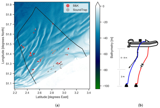
Figure 1.
(a) Data collected, colored according to instrument used. The background represents the bathymetry from the EMODnet bathymetry. The solid black line represents the borders of the Belgian Exclusive Economic Zone; (b) Deployment scheme for two instruments simultaneously. The left instrument setup (blue rope) is the B and K. The black squared box represents the Nexus amplifier and the DR-680 TASCAM recorder attached to the B and K system. The right instrument (red rope) is the SoundTrap.
In this study, a deployment was defined as a measurement interval corresponding to the time when a hydrophone was in the water, without changing any recording parameters or rope length. Each of the deployments consisted of 30 to 60 min of continuous recording, following the current by drifting, with the engines and the plotter turned off, to reduce the noise created by the boat itself. The typical drifting speed was 1 ms. During each deployment, a GPS Garmin with a time resolution of 1s stored the location during the entire deployment, and was synchronized with the instrument clock. The length of the rope was chosen according to the depth, so that the hydrophone would be, on average, between the 1/2 and 1/3 of the water column from the surface (see Figure 1b). The rope length was kept constant during each entire deployment, and it was considered the instrument depth. The instruments used were a SoundTrap ST300HF (Ocean Instruments, Auckland, New Zealand) (sensitivity: 172.8 dB re 1 V/Pa—from now on, SoundTrap) and a Bruel and Kjaer Nexus 2690, with a hydrophone type 8104 (Bruel and Kjaer, Virum, Denmark) (sensitivity: 205 dB re 1 V/Pa—from now on, B and K) together with a DR-680 TASCAM recorder. The amplification in the Nexus was set to 10 mV, 3.16 mV or 1 mV, depending on the loudness of the recording location. The SoundTrap was set to sample at 560 ksps, and the B and K at 192 ksps.
Of the 40 independent tracks recorded, 14 were recorded simultaneously, with two different devices, to confirm their interchangeability: this made for a total of 54 deployments (Figure 1). The metadata were stored in the online repository of the European Tracking Network, under the Underwater Acoustics component (ETN, https://www.lifewatch.be/etn/ (accessed on 19 January 2023)).
2.2.2. Acoustic Processing
Acoustic changes in the soundscape were expected to be found in a small spatial (meters) and temporal (seconds) resolution: for this reason, the data were processed in time windows of 1 s (hereafter, ), with no overlap. Then, these 1-second bins, , were arranged in groups of 5, with an overlap of 60%, (hereafter, ) (Equation (1)). The time window and the overlap were chosen so that the spatial resolution would be of 2 samples every 5 m, considering an average drifting speed of 1 ms.
All the acoustic processing was done using pypam [44], an open-source python tool for processing acoustic files in chunks. Each recorded file was converted to sound pressure, using the calibration factor for the equipment used. For the SoundTrap, the calibration was done according to the value given by the manufacturer. The B and K equipment was calibrated by generating a calibration tone at the beginning of each file, and was afterwards removed from the file. The rest of the recording was processed according to the obtained calibration value. The sound pressure values obtained by the two instruments recording simultaneously were compared, to make sure the calibrations were accurate. Per time window, a Butterworth band pass filter of order 4 was applied between 10 and 20,000 Hz, and the signal was down-sampled to twice the high limit of the filtered band. The frequency band was chosen to cover all the biophony and geophony of interest for this study that we could record, given the sampling frequency limitations of the equipment. After filtering, the root mean squared value of the sound pressure of each one-third octave band (base 2) was computed per each 1-second bin . Then, every 5 s were joined, to create an acoustic sample, , which resulted in 5 × 29 one-third octave bands per time window (1). Each sample was flattened to an array of 145 × 1, for further analysis. One-third octave bands were chosen because of their availability and commonness, and because they are considered to be appropriate for most considerations of environmental impact [45]. Furthermore, they had previously been used to describe soundscapes [46,47,48].
2.2.3. Environmental Data
Each acoustic sample, , was matched to the closest point in time stored in the GPS tracker. If did not have a GPS point closer than 5 s in time, it was eliminated from the dataset. All available environmental data in the BPNS were reviewed, and the selected environmental parameters are shown in Table 1. The list of all the considered parameters is referred to as in Figure 2.

Table 1.
Summary of the all the available environmental variables.
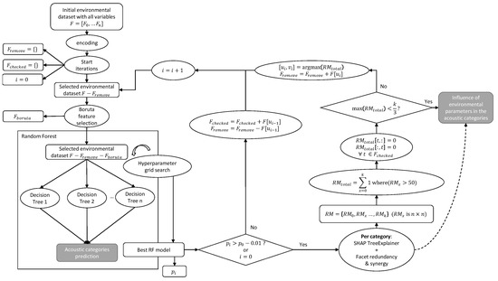
Figure 2.
Diagram of the trained Random Forest and the environmental characteristics assessment: k is the number of categories; i is the iteration number; F are all the available variables; n is the number of available variables; is the performance of iteration i; is the redundancy matrix , with the “perspective” feature as rows; the dashed line illustrates the basis of the influence.
The selected environmental data were paired to each sample, , using the python package bpnsdata [49]. We will refer to the environmental data paired to sample as . Some data were not available in the public environmental datasets during some of the recording periods, so any with a corresponding incomplete was also removed from the dataset.
The cyclic variables, season and moon phase, were split into their cosine and their sine values, with the intention of representing the cyclic continuation of the values. Categorical variables were encoded using the one-hot-encoder function of sklearnDF [50]. Distance to closest shipwreck was converted into logarithmic scale, as its effect was expected to be relevant only at a very close distance, because of the short propagation of the calls of the expected benthic fauna [51]. The decay of sound pressure with distance was expected to be around , and we therefore used the logarithm to linearize. Bathymetry was converted to a positive value. See Table 1 for more details.
2.3. Acoustic Categorization
2.3.1. Dimension Reduction and Acoustic Dissimilarity
A dimension reduction algorithm was applied to the acoustic data. For the outcome to show changes in clusters in a visual way, 2-D was chosen as an appropriate number of dimensions. Uniform Manifold Approximation and Projection (UMAP) was considered appropriate for dealing with the non-linearity of the data [59]. UMAP is a dimension reduction technique that can be used for visualization, similar to t-SNE [60], but also as a general non-linear dimension reduction tool. It models the manifold with a fuzzy topological structure. The embedding is found by searching for a low dimensional projection of the data, which has the closest possible equivalent fuzzy topological structure. UMAP was preferred over t-SNE, because it better preserves the global structure of the data [61]. Different configurations of the UMAP parameters were tested, to try to achieve an optimal distribution of the data, where acoustic sample points were distributed in separated clusters. Using UMAP, the data were represented by more similar points closer to each other, and by more different points further apart: the idea was to exaggerate local similarities, while also keeping a structure for global dissimilarities.
Similar sounds were thus expected to create clusters, and clusters further apart to represent more different sounds than clusters closer together, in the 2D space [28]. The 2D dimension could then be used to compute distances between clusters, as a measure of acoustic dissimilarity between two groups of sounds. However, not all of these clusters represented a soundscape, because specific sounds which had occurred in the dataset multiple times, but were not related to their recording location or time, also formed clusters; therefore, some of the obtained clusters might not represent a soundscape, but only a certain foreground sound. We tackled this distinction using XAI, and we considered soundscape-clusters to be the ones closely linked to the environmental parameters. Clusters not correlated to the environmental parameters were not considered to be soundscape classes in this study.
2.3.2. Data Cleaning: Artifacts Removal
During underwater acoustic deployments, a lot of artifacts can affect the recordings: these do not contain any ecologically relevant information, nor do they mask existing information, and thus they need to be removed. They can be caused by small particles hitting the hydrophone, or by sounds generated by the deployment structure or the instrument itself. In this study, a semi-supervised approach was applied, to remove the artifacts. All the recordings made with the B and K equipment were manually checked for artifacts segments, and were annotated in a non-detailed fashion. Visual inspections of 10-minute spectrograms were conducted in Audacity [62], and artifacts that were clearly visible were annotated. Each annotation comprised the start and end of the artifact event, and the designated label: clipping; electronic noise; rope noise; calibration signal; and boat noise. All the samples which contained more than 1 s of artifact data were labeled with the corresponding tag.
These labels were then plotted in the UMAP space, to check visually if there was any visible clustering. Then, all the data embedded in the 2D space were clustered using Density-Based Spatial Clustering of Applications with Noise (DBSCAN), using the scikit-learn package [63]. This algorithm finds core samples of high density, and expands clusters from them: it is appropriate for data which contain clusters of similar density. Samples that were not close enough to any cluster were considered “noise”, and therefore could not be classified as one particular class. After clustering, the percentage of artifact samples in each of the resulting clusters was assessed. If the ratio of artifact samples in that cluster exceeded 2 times the ratio of total samples labeled as artifacts in the dataset (Equation (2)), it was considered to be an artifact-cluster, and was therefore removed from the dataset. Consequently, all the samples that were clustered in an artifact-cluster, but which had not been manually labeled as artifacts, were also considered artifacts (Figure 3). The DBSCAN “noise” class was also considered a cluster, and treated accordingly.
where represents the samples classified as cluster i, and underscore artifacts means samples classified as any of the artifact labels.
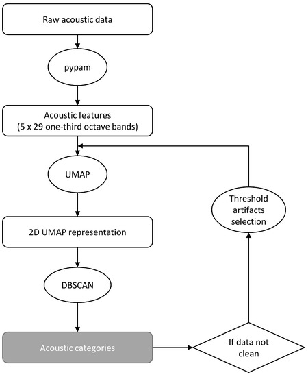
Figure 3.
Flowchart to obtain the acoustic categories.
2.3.3. Acoustic Categories
The UMAP dimension reduction was applied for a second time, to the clean dataset: this was done because the artifact clusters were expected to be acoustically very dissimilar to the environmental clusters; therefore, re-computing the UMAP without them would help obtain clearer distinctions between environmental clusters. The data obtained in the new, embedded 2D space were clustered again, using DBSCAN. Samples classified as noise were removed from the analysis, as they were considered outliers, and could not be classified as one particular acoustic category. The obtained classes after the noise reduction were considered as the different acoustic categories present in the dataset. A diagram of the workflow for artifact removal and final clustering can be seen in Figure 3.
2.4. Characterization of Acoustic Classes
To understand which environmental parameters were correlated to the categorized acoustic environments (clusters), and could be used to describe them, a Random Forest (RF) Classifier was built, with the environmental variables as the independent variables, and the obtained acoustic clusters as the dependent variable. The input variables were encoded, as described in Section 2.2.3. The RF was subsequently analyzed, using the XAI inspector system from the FACET gamma package, which is based on SHAP (SHapley Additive exPlanations) [64]. SHAP is a method of explaining individual predictions of instance X, by computing the contribution of each feature to the prediction. The SHAP explanation method can be used to understand how each feature affects the model decisions, by generalizing local relationships between input features and model output. The python SHAP library contains an algorithm called TreeExplainer, made specifically to interpret tree-based Machine Learning models [65]. For this analysis, the TreeExplainer approach was used, considering a marginal distribution (interventional feature perturbation). However, the output of the SHAP analysis can give misleading conclusions if redundant variables are present in the dataset, because the importance of variables that share information will be split between them, as their contribution to the model is also split: the real impact of that redundant pair—and the ecological phenomena they represent—will therefore not be assessed. To overcome this problem, the model was evaluated for redundancy between variables [66]. In facet-gamma, redundancy quantifies the degree to which the predictive contribution of variable u uses information that is also available through variable v. Redundancy is a naturally asymmetric property of the global information that feature pairs have for predicting an outcome, and it ranges from 0% (full uniqueness) to 100% (full redundancy).
The RF was trained multiple times in an iterative way, where one of the possible redundant variables was removed at each iteration, as displayed in Figure 2. At the start of each iteration, the Boruta algorithm [67] was used, to check if any of the variables were not relevant. Then, to find out the best hyper-parameters for the algorithm, a grid search with cross-validation with 5 folds was run on all the data, with accuracy as the scoring metric. The parameters of the grid can be seen in Table A4. The results given for all the models are considering the cross-validation approach.
To decide if a variable should be removed from the analysis because it was too redundant, the obtained best RF was evaluated for each class, using the FACET [68] package. First, the redundancy matrix was computed per class [68]. Then, we counted in how many classes a variable pair was more than 50% redundant. The pair exceeding the threshold in the highest number of classes was selected for removal, and the “perspective” variable was removed from the dataset in the following iteration. The whole training process was repeated without this variable, and the accuracy of the model was compared to the model from the first iteration. If the performance did not decrease by more than 1%, the variable was excluded from all further iterations. If the performance decreased more than 1%, then the variable was considered too important to be removed, was kept, and was not checked anymore in the following iterations. Iteratively, this process was repeated, until there were no pairs that had a redundancy higher than 50% in more than 1/3 of the classes. The last best RF model obtained was used for further analysis, with all the redundant features already eliminated.
Once all the redundant variables were removed, the last RF model was interpreted, using SHAP to further depict the relative importance of the remaining environmental features, to characterize the acoustic clusters. Using the computed SHAP values, a summary of the most important global features was plotted and analyzed. The SHAP python package incorporates the option to produce beeswarm plots, which allow for checking for feature importance per category, and understanding which values of each feature increase or decrease the probability of belonging to a certain class; therefore, the SHAP values were plotted per category individually: this allowed for assessing why a certain spatiotemporal location was classified as a certain type of acoustic category.
SHAP offers an interactive plot, whereby we can see the probability contribution of each feature per class in time. In these plots, we can visualize the shapely values of each feature value as a force (arrow) that pushes to increase (positive value) or decrease (negative value) the probability of belonging to that specific class.
To test if the deployment settings had a significant influence on the recorded soundscapes, a categorical variable representing each deployment (deployment_id) was added, and the whole process was repeated. The selected variables were compared, and the influence of the deployment_id was compared to the other variables. The performance (total of data explained) of the RF trained with the deployment_id variable was compared to the model obtained, using only environmental variables. If the performance of the model did not improve by adding the deployment_id variable, it was assumed that it was redundant, with the data being already present in the dataset.
Furthermore, to understand whether there were specific clusters that were not understood by the model, because they represented a certain sound not directly linked to the available environmental parameters, the data incorrectly classified by the obtained RF model was plotted in the 2D space, to visually check if the samples wrongly classified grouped together. The percentage of each cluster correctly explained by the model was computed.
3. Results
3.1. Data
In total, 54 tracks were recorded during 10 different days, yielding a total of 40 h 47 min of acoustic data (see Figure 1). After merging the acoustic data with the environmental data, due to some missing data the dataset was reduced to 42,117 samples ().
3.2. Acoustic Categorization
3.2.1. Data Cleaning
A total of 107 artifacts were manually labeled. The labeled data were plotted in a 2D UMAP representation, clearly grouped according to the label (Figure 4), which highlighted that points closer to each other in the UMAP space were similar acoustically (Table A2 for details). The DBSCAN algorithm generated 37 clusters (Table A3 for details): from these clusters, 9 were considered artifacts, and were removed from the dataset. The sum of all the samples of these clusters represented 15.30% of the dataset.
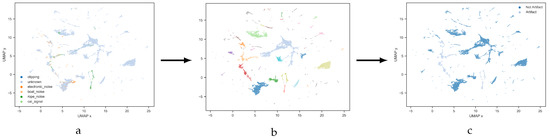
Figure 4.
(a) distribution of the labeled artifacts on the 2D UMAP dimension; (b) obtained 37 clusters after applying DBSCAN; (c) data considered to be artifact.
3.2.2. Acoustic Categories
UMAP was applied to the dataset without artifacts for a second time. The clean data plotted in this second UMAP space also presented clear clusters (Figure 5 and Table A2 for details).
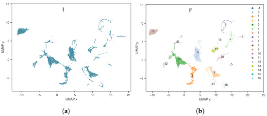
Figure 5.
(a) dimension reduction, using UMAP on the clean dataset; (b) obtained clusters using UMAP projection: −1 represents the noise class.
A DBSCAN algorithm was run on the new UMAP space, and 17 clusters were obtained (Table A3). Of the samples, 6.01% were classified as noise, and therefore they were removed from the dataset, for further analysis (Figure 5). The mean and standard deviations of each cluster’s one-third octave bands evolution can be seen in Table A5.
3.3. Characterization of Acoustic Classes
During the Boruta analysis, seabed_habitat_A5.23 or A5.24 was selected for removal. All the results of the iterative training of the RF and the redundant variables removal are summarized in Table 2. In the final model temperature, new_moon, substrate_Sandy mud to muddy sand and week_n_cos were removed.
Table 2.
Summary of the selected model at each iteration, and their performance with the consequent redundant pairs and the features removed.
The accuracy from the last best RF trained was 91.77%: this percentage represented the proportion of the data that could be explained by the model. In the visual analysis of the data incorrectly classified, it was seen that the data incorrectly classified clearly clustered or were at the border of a cluster (Figure 6): this supported the hypothesis that these clusters represented similar sounds not correlated to the considered environmental parameters. After computing the percentage of each cluster correctly predicted by the model, cluster 14 was discarded as a soundscape, because 0% of its samples were correctly explained by the environmental variables.
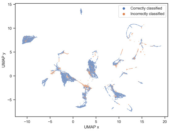
Figure 6.
Samples correctly and incorrectly classified using the RF obtained in the last iteration.
Using the last RF, the SHAP values were computed for the total dataset. The parameters most distinctive between classes globally were day_moment, instrument_depth, coast_dist, salinity and growing_moon (Figure 7). With the obtained plots of SHAP values per class, it could be understood which values were affecting each class. For example, from Figure 8, it can be interpreted that high values of instrument_depth increased the probability of a sample belonging to class 0. With coast_dist it was the other way around, and lower values decreased the probability of a sample belonging to class 0. For class 1, low values of shipping increased the probability of belonging to class 1, and high values of instrument_depth likewise. The SHAP plots per category can be see in Figure A1, and the results are manually summarized in Table 3. To improve visualization, variables corresponding to an encoded value of a categorical variable were grouped, and plotted in gray in the SHAP plots: this was done because categorical variables do not have higher and lower values. In all the interpretations, medium values of week_n_cos were considered summer, because there was no sampling done in winter.
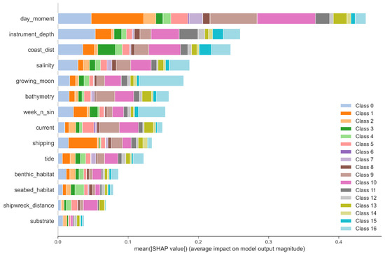
Figure 7.
Global summary of the influence of the environmental parameters on the acoustic categorization in the entire dataset.
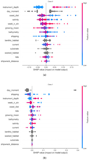
Figure 8.
Summary of the SHAP values for all the environmental parameters for (a) class 0 (b) class 1. The summary of SHAP values for other classes can be seen on Figure A1. Variables in gray are categorical variables.
Table 3.
Manual interpretation of the influence of the environmental variables in cluster differentiation. Because there was no sampling done in winter, medium values of week_n_cos were considered summer.
The total performance of the model, when adding the deployment_id variable, did not improve. It was concluded that deployment_id could safely be removed, and not considered a necessary factor to explain the differences between acoustic categories.
We manually analyzed the output categories in space and time. We observed a variation in the soundscapes recorded across the 40 sites, and also a shift within some individual deployments. The changes were driven by both spatial and temporal features: as an example, we examined a location recorded during different days and moments (Figure 9). The deployment plotted in (a)–(b) fell mostly under class 0, which was characterized as spring. The deployment in (c)–(d) fell under class 1, which was characterized as autumn.
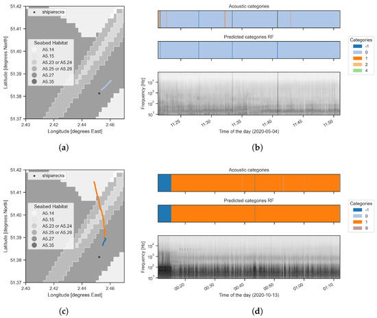
Figure 9.
Deployment in spring plotted spatially (a) and temporally (b). Deployment in autumn, plotted temporally (c) and spatially (d).
Some deployments changed soundscape categories during the deployment, as in Figure 10, in which the deployment started with class 3, then switched to class 13, and then to class 6. Referring to Table 3 and Figure A1, the biggest differences between class 3 and classes 13 and 6 were the current and distance to a shipwreck. This description correlates with the fact that the current was lower when class 3 appeared, and higher during classes 13 and 6. It also correlates with the fact that there was a shipwreck close to class 3, while there were no shipwrecks in the vicinity of class 6 and 13. Furthermore, the change of cluster from class 13 to class 6 may have been due to the change in the sea bottom substrate, where it changed from coarse sediment to sand. These descriptions match the spatial changes (Figure 10a), where class 13 was found usually on coarse sediment bottoms, and class 6 was not defined by the substrate. In the spectrogram, we can also see a clear change in the sound, and some of the last parts were classified as noise, because of the loud shipping noise present. In this particular example, the first time that class 6 appeared for a short time at 11:40, it was not correctly predicted by the model. The same happened with the small jump to class 14, which was not considered a soundscape, and therefore was just a foreground event not considered by the model. Other examples of deployments can be found in Figure A2.
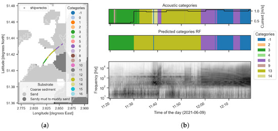
Figure 10.
Zoom of one deployment recorded the 9 June of 2021: (a) plotted on top of a map of the substrate type; (b) plotted in time.
In Figure 11, we can see the interactive "force" plots for the dominant classes from the same deployment as Figure 10, where it is shown how the model predicts these classes over time.
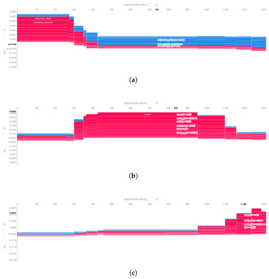
Figure 11.
SHAP plots showing samples’ probability of belonging to classes 3 (a), 13 (b) and 6 (c). The x axis is the time in samples; the y axis is the probability of a sample to be classified as a specific class. Blue probabilities are negative influences, and red probabilities are positive influences of a variable.
4. Discussion
In this study, we showed that by using an unsupervised approach we were able to categorize different marine shallow water soundscapes. In addition, we demonstrated that by using an automatic (supervised) approach, based on Explainable machine learning tools, we were able to characterize these categories ecologically. Our method was able to group soundscapes in different categories, which could be used to understand the spatiotemporal acoustic variations of a dataset. The obtained categories were afterwards proved to be connected to environmental parameters through an RF classifier. To understand the predictions made by the trained RF, SHAP values were used: this allowed for the assessment of the main environmental parameters shaping the acoustic categories in general, but also per category, which provided a practical ecological profile for each soundscape category.
Our results show that the acoustic data analyzed by UMAP and DBSCAN clustered mostly in clear, independent groups. This indicates that there were major and quantifiable differences in BPNS’ underwater soundscapes, and that one-third octave bands encoded enough information to capture these dissimilarities. This was an advantage, due to the current availability of built-in implementations in some recorders, and the different available tools to compute them. We chose the frequency band of study to capture the sound sources of interest, but increasing the frequency range could lead to new clusters. The chosen frequency band captured enough information to obtain distinct clusters, even though increasing the frequency range might have increased the number of clusters. Furthermore, similar artifact sounds clustered together. This was in line with findings from Sethi et al. (2020), where artifacts could be detected by using an unsupervised clustering technique. Accordingly, the semi-supervised process used in this study could be applied to detecting artifacts in acoustic datasets. This would be especially useful for long-term deployments, where exhaustive manual analysis is too time consuming, and it would be a rapid solution for detecting instrument malfunction events.
The RF classifier was able to correctly classify more than 90% of the BPNS’ acoustic data into the 17 relevant soundscape categories: this high accuracy suggests that the environmental parameters included in the analysis were good indicators of the observed acoustic patterns. The SHAP values showed that in our case study, time of the day, instrument depth, distance to the coast, salinity and moon phase were the most important environmental parameters shaping and differentiating the soundscape categories. These results should be carefully interpreted. The importance of the environmental parameters was not necessarily correlated to their influence on the total sound: rather, it described their relevance to discriminating between categories. For example, if all the categories from the study area had had a considerable and equally distributed sound contribution from shipping, the feature would not have had a great effect in differentiating them: as a consequence, it would have had a low importance score in the model. However, if we had expanded the dataset with acoustic data from other areas in the world with less shipping influence, shipping would have become a very dominant feature in explaining the categories’ differences. In addition, the redundant variables that were removed should not be ignored, but should be considered together with the redundant pair. For example, temperature was removed, because of its redundancy with the season (week_n_sin). Consequently, in all the clusters where season has an influence, we would not be able to distinguish if the real effect was the temperature or the season: we would know, however, that these two correlated parameters had an influence on the soundscape. If distinguishing between two redundant features would be relevant, more data should be collected to that effect, in a way that the two variables are not correlated.
Instrument depth showed a strong influence on discriminating between soundscape categories. This result could have been expected: as the recording depth was not kept at the same level and in such shallow environments, acoustic changes in the soundscape occurred at very small spatial scales, and vertically in the water column [45]. It is therefore important to always consider and report the hydrophone depth when comparing different soundscapes, to avoid any misleading conclusions. Furthermore, to exclude the position effect, and in order to better assess the biotic-driven soundscapes in shallow environments, recordings should be taken at a fixed depth.
The obtained categories showed the expected acoustic variation: this reflected the dynamic environment in the BPNS, and the need to study these soundscapes in more detail, in order to better understand this specific marine acoustic environment. Spatial or temporal change in environmental variables could be noticed in the acoustic scenes, and the obtained categories reflected these changes. In general, a greater proportion of spatial environmental parameters were determined to be important by the RF model: this was most likely explained by the fact that we did not record over long periods of time (e.g., over all four seasons or years) and, therefore, many biotic acoustic patterns that are known to be temporally driven [69] were not completely captured in our dataset.
Future work should hold the same analysis on a more extensive dataset with stationary recording stations, such as the dataset from the LifeWatch Broadband Acoustic Network [70]. This would allow for testing the potential to capture circadian, monthly or seasonal cycles. To be able to generalize our conclusions and test the robustness of the method, it should be applied to new long- and short-term data from different underwater acoustic contexts. If these datasets came from ecosystems that were well-studied acoustically, the results would be contrasted. We would thereby be able to assess whether the obtained categories were representative and informative enough, and if they matched the currently existing knowledge or if they complemented it. Furthermore, the incorrectly classified data could also be analyzed manually, to detect specific events, and to have more insight into the missing explanatory parameters.
The method proposed here could be particularly useful in environments where the visual correlation between ecological factors and the underwater soundscape cannot be established: this includes low visibility and other challenging conditions, such as those occurring in remote areas with high latitudes, where the winter season prevents traditional ways of surveying, or in highly exploited areas. In these cases, a rapid and automated tool, capable of characterizing the soundscape, and of monitoring its potential changes in relation to relevant environmental drivers, would be very valuable.
Ecologically characterizing the soundscape categories is only possible if data from all the environmental parameters are available. If not, the method could still be applied to categorize the different recorded soundscapes into acoustically relevant categories that could help guide conservation decisions on, e.g., areas with diver soundscape patterns. It would also be possible to use the categories to optimize the sampling effort, and to only sample for potential drivers where the soundscape categories are, e.g., most distinct. If no environmental data from a specific site were available, it would be possible to train the model on a similar dataset, but with available environmental data. The acoustic data could then be explored, according to the obtained classification, to assess whether there were similarities between the soundscape categories obtained in both datasets, thus establishing a potential relationship with analogous drivers. In addition, the acoustic categories obtained in such an unsupervised way could be manually analyzed and labeled, and subsequently used as a baseline for future monitoring, to assess the acoustic change in time or the spatial acoustic (dis)similarities in a certain environment.
5. Conclusions
Our work constitutes a significant contribution to the development of a methodology for monitoring and characterizing underwater soundscapes in a fast and automatic way, thereby complementing previous works on underwater soundscape analysis [71,72,73].
Classifying soundscapes into categories assigns a label to each acoustic environment: this is an easy way to refer to and identify them, which can be useful for policy or conservation programs. One application of using categories is to analyze long-term data. The categories are able to point out trends, status and seasonal patterns. Working with fully unsupervised acoustic categories creates the potential to assess the dynamic character of the soundscape. The fact that no labeling effort is needed is a step towards solving the problem of coping with the analysis of the increasing amount of acoustic data that the technological advances allow to be collected and stored. In the global context of rapid environmental change and increasing anthropic pressure, it is of critical importance to assess the acoustic research gap, and to study bias towards more accessible ecosystems [2]. The method we propose here constitutes an innovative and practical tool for categorizing and characterizing marine soundscapes, particularly in poorly known acoustic contexts. It could be used for conservation purposes, disturbance detection and ecosystem integrity assessment.
Author Contributions
Conceptualization, C.P., I.T.R., E.D., D.B. and P.D.; methodology, C.P., I.T.R., E.D., D.B. and P.D.; software, C.P.; formal analysis, C.P.; investigation, C.P. and E.D.; resources, E.D.; data curation, C.P.; writing—original draft preparation, C.P.; writing—review and editing, I.T.R., E.D., D.B. and P.D.; visualization, C.P.; supervision, E.D., D.B. and P.D.; project administration, E.D.; funding acquisition, E.D. All authors have read and agreed to the published version of the manuscript.
Funding
This research was funded by LifeWatch grant number I002021N.
Institutional Review Board Statement
Not applicable.
Informed Consent Statement
Not applicable.
Data Availability Statement
The dataset of the processed acoustic data (one-third octave bands) can be found in the Marine Data Archive (https://doi.org/10.14284/586 (accessed on 19 January 2023)).
Acknowledgments
The project was realized as part of the Flemish contribution to LifeWatch. We would like to thank the crew of the RV Simon Stevin. We would also like to thank Jan Vermaut for his essential work in driving the Zeekat drifting all over the BPNS, and the Sailawaywithme sailing team who made it possible to sail to further places and acquire night recordings. We would also like to acknowledge the contribution of Roeland Develter and Klaas Deneudt, for helping with the data collection. The author would also like to thank Peter Rubbens and Olaf Boebel for their advice during the study, and Marine Severin for her help with the manuscript.
Conflicts of Interest
The authors declare no conflict of interest.
Abbreviations
The following abbreviations are used in this manuscript:
| BPNS | Belgian Part of the North Sea |
| XAI | Explainable Artificial Intelligence |
| PAM | Passive Acoustic Monitoring |
| B and K | Bruel and Kjaer |
| RF | Random Forest |
| UMAP | Uniform Manifold Approximation and Projection |
| DBSCAN | Density-Based Spatial Clustering of Applications with Noise |
| SHAP | SHapley Additive exPlanations |
Appendix A
Table A1.
Summary of all the field work days and the equipment used.
Table A1.
Summary of all the field work days and the equipment used.
| Date | Boat | Shipwrecks | SoundTrap | B and K |
|---|---|---|---|---|
| 27 April 2020 | RIB Zeekat | Coast, Loreley, Nautica Ena, Noordster, Paragon, Renilde | 576 kSs | NA |
| 29 April 2020 | RIB Zeekat | Heinkel 111, HMS Colsay, Lola, Westerbroek | 576 kSs | 192 kSs |
| 5 May 2020 | RIB working boat from RV Simon Stevin. | Buitenratel, Killmore, Westhinder | NA | 192 kSs |
| 13 July 2020 | RIB working boat from RV Simon Stevin. | Faulbaums, Grafton | NA | 192 kSs |
| 6 May 2020 | RIB working boat from RV Simon Stevin. | Belwind, CPower | NA | 192 kSs |
| 7 May 2020 | RIB working boat from RV Simon Stevin. | Garden City | NA | 192 kSs |
| 8 May 2020 | RIB working boat from RV Simon Stevin. | G88, Loreley, Nautica Ena, Paragon | NA | 192 kSs |
| 1 to 3 June 2020 | Sailing boat Capoeira. | Birkenfels, Buitenratel, Gardencity, Grafton, Nautica Ena, VG, Westhinder, WK8 | NA | 192 kSs |
| 12 to 13 October 2020 | Sailing boat Capoeira. | Birkenfels, Buitenratel, Faulbaums, Garden city, Grafton, Nautica Ena, VG, Westhinder, WK8 | NA | 192 kSs |
| 9 to 10 June 2021 | Sailing boat Capoeira. | Birkenfels, Buitenratel, Faulbaums, Garden City, Grafton, Nautica Ena, Noordster, VG2, Westhinder, WK8 | 576 kSs | 192 kSs |
Table A2.
Parameters used for UMAP dimension reduction.
Table A2.
Parameters used for UMAP dimension reduction.
| Dataset | Selected Minimum Distance | Selected Number Neighbors |
|---|---|---|
| Full | 0.0 | 10 |
| Clean | 0.0 | 50 |
Table A3.
Parameters used for DBSCAN.
Table A3.
Parameters used for DBSCAN.
| Dataset | Selected Minimum Samples | Selected Epsilon |
|---|---|---|
| Full | 100 | 0.5 |
| Clean | 720 | 0.9 |
Table A4.
Parameters used for the grid search during hyper-parameter tuning for the training of the RF.
Table A4.
Parameters used for the grid search during hyper-parameter tuning for the training of the RF.
| Parameter | Values |
|---|---|
| criterion | gini, entropy |
| min_samples_split | 100, 300, 500 |
| max_depth | 6, 8, 12 |
| min_samples_leaf | 100, 200, 300 |
| max_leaf_nodes | 10, 15, 20 |
Table A5.
Mean and standard deviations of the values of the one-third octave bands, in time per each category.
Table A5.
Mean and standard deviations of the values of the one-third octave bands, in time per each category.
| Cluster | Acoustic Summary |
|---|---|
| 0 |  |
| 1 |  |
| 2 |  |
| 3 |  |
| 4 |  |
| 5 |  |
| 6 |  |
| 7 |  |
| 8 |  |
| 9 |  |
| 10 |  |
| 11 |  |
| 12 |  |
| 13 |  |
| 14 |  |
| 15 |  |
| 16 |  |
| 17 |  |


Figure A1.
Summary of the SHAP values for all the features for class: (a) 0 (b) 1 (c) 2 (d) 3 (e) 4 (f) 5 (g) 6 (h) 7 (i) 8 (j) 9 (k) 10 (l) 11 (m) 12 (n) 13 (o) 14 (p) 15 (q) 16.

Figure A2.
Examples of deployments evolution in time, recorded on the (a) 9 June 2021 (b) 8 May 2020 (c) 4 May 2020 (d) 7 May 2020 (e) 9 June 2021 (f) 29 April 2020.
References
- Schoeman, R.P.; Erbe, C.; Pavan, G.; Righini, R.; Thomas, J.A. Analysis of Soundscapes as an Ecological Tool. In Exploring Animal Behavior Through Sound: Volume 1: Methods; Erbe, C., Thomas, J.A., Eds.; Springer International Publishing: Cham, Switzerland, 2022; pp. 217–267. [Google Scholar] [CrossRef]
- Havlik, M.N.; Predragovic, M.; Duarte, C.M. State of Play in Marine Soundscape Assessments. Front. Mar. Sci. 2022, 9, 919418. [Google Scholar] [CrossRef]
- Krause, B.; Farina, A. Using Ecoacoustic Methods to Survey the Impacts of Climate Change on Biodiversity. Biol. Conserv. 2016, 195, 245–254. [Google Scholar] [CrossRef]
- Pijanowski, B.C.; Villanueva-Rivera, L.J.; Dumyahn, S.L.; Farina, A.; Krause, B.L.; Napoletano, B.M.; Gage, S.H.; Pieretti, N. Soundscape Ecology: The Science of Sound in the Landscape. BioScience 2011, 61, 203–216. [Google Scholar] [CrossRef]
- ISO 18405:2017; Underwater acoustics—Terminology. International Organization for Standardization: Geneva, Switzeland, 2017.
- Gibb, R.; Browning, E.; Glover-Kapfer, P.; Jones, K.E. Emerging Opportunities and Challenges for Passive Acoustics in Ecological Assessment and Monitoring. Methods Ecol. Evol. 2019, 10, 169–185. [Google Scholar] [CrossRef]
- Duarte, C.M.; Chapuis, L.; Collin, S.P.; Costa, D.P.; Devassy, R.P.; Eguiluz, V.M.; Erbe, C.; Gordon, T.A.C.; Halpern, B.S.; Harding, H.R.; et al. The Soundscape of the Anthropocene Ocean. Science 2021, 371, eaba4658. [Google Scholar] [CrossRef] [PubMed]
- Do Nascimento, L.A.; Campos-Cerqueira, M.; Beard, K.H. Acoustic Metrics Predict Habitat Type and Vegetation Structure in the Amazon. Ecol. Indic. 2020, 117, 106679. [Google Scholar] [CrossRef]
- Dröge, S.; Martin, D.A.; Andriafanomezantsoa, R.; Burivalova, Z.; Fulgence, T.R.; Osen, K.; Rakotomalala, E.; Schwab, D.; Wurz, A.; Richter, T.; et al. Listening to a Changing Landscape: Acoustic Indices Reflect Bird Species Richness and Plot-Scale Vegetation Structure across Different Land-Use Types in North-Eastern Madagascar. Ecol. Indic. 2021, 120, 106929. [Google Scholar] [CrossRef]
- Ainslie, M.A.; Dahl, P.H. Practical Spreading Laws: The Snakes and Ladders of Shallow Water Acoustics. In Proceedings of the Second International Conference and Exhibition on Underwater Acoustics, Providence, RI, USA, 5–9 May 2014; p. 8. [Google Scholar]
- McKenna, M.F.; Baumann-Pickering, S.; Kok, A.C.M.; Oestreich, W.K.; Adams, J.D.; Barkowski, J.; Fristrup, K.M.; Goldbogen, J.A.; Joseph, J.; Kim, E.B.; et al. Advancing the Interpretation of Shallow Water Marine Soundscapes. Front. Mar. Sci. 2021, 8, 719258. [Google Scholar] [CrossRef]
- Miksis-Olds, J.L.; Martin, B.; Tyack, P.L. Exploring the Ocean Through Soundscapes. Acoust. Today 2018, 14, 9, 26–34. [Google Scholar]
- Mueller, C.; Monczak, A.; Soueidan, J.; McKinney, B.; Smott, S.; Mills, T.; Ji, Y.; Montie, E. Sound Characterization and Fine-Scale Spatial Mapping of an Estuarine Soundscape in the Southeastern USA. Mar. Ecol. Prog. Ser. 2020, 645, 1–23. [Google Scholar] [CrossRef]
- International Organization for Standardization (ISO). Acoustics—Soundscape—Part 1: Definition and Conceptual Framework; Technical Report; International Organization for Standardization (ISO): Geneva, Switzerland, 2014. [Google Scholar]
- Abeßer, J. A Review of Deep Learning Based Methods for Acoustic Scene Classification. Appl. Sci. 2020, 10, 2020. [Google Scholar] [CrossRef]
- IQOE—Inventory of Existing Standards and Guidelines Relevant to Marine Bioacoustics; Technical Report; IQOE: Neuchatel, Switzerland, 2021.
- Sethi, S.S.; Ewers, R.M.; Jones, N.S.; Sleutel, J.; Shabrani, A.; Zulkifli, N.; Picinali, L. Soundscapes Predict Species Occurrence in Tropical Forests. Oikos 2021, 2022, e08525. [Google Scholar] [CrossRef]
- Schoeman, R.P.; Erbe, C.; Plön, S. Underwater Chatter for the Win: A First Assessment of Underwater Soundscapes in Two Bays along the Eastern Cape Coast of South Africa. J. Mar. Sci. Eng. 2022, 10, 746. [Google Scholar] [CrossRef]
- Nguyen Hong Duc, P.; Cazau, D.; White, P.R.; Gérard, O.; Detcheverry, J.; Urtizberea, F.; Adam, O. Use of Ecoacoustics to Characterize the Marine Acoustic Environment off the North Atlantic French Saint-Pierre-et-Miquelon Archipelago. J. Mar. Sci. Eng. 2021, 9, 177. [Google Scholar] [CrossRef]
- Sueur, J.; Farina, A.; Gasc, A.; Pieretti, N.; Pavoine, S. Acoustic Indices for Biodiversity Assessment and Landscape Investigation. Acta Acust. United Acust. 2014, 100, 772–781. [Google Scholar] [CrossRef]
- Buxton, R.T.; McKenna, M.F.; Clapp, M.; Meyer, E.; Stabenau, E.; Angeloni, L.M.; Crooks, K.; Wittemyer, G. Efficacy of Extracting Indices from Large-Scale Acoustic Recordings to Monitor Biodiversity. Conserv. Biol. 2018, 32, 1174–1184. [Google Scholar] [CrossRef]
- Sueur, J.; Pavoine, S.; Hamerlynck, O.; Duvail, S. Rapid Acoustic Survey for Biodiversity Appraisal. PLoS ONE 2008, 3, e04065. [Google Scholar] [CrossRef]
- Pieretti, N.; Lo Martire, M.; Farina, A.; Danovaro, R. Marine Soundscape as an Additional Biodiversity Monitoring Tool: A Case Study from the Adriatic Sea (Mediterranean Sea). Ecol. Indic. 2017, 83, 13–20. [Google Scholar] [CrossRef]
- Bertucci, F.; Parmentier, E.; Lecellier, G.; Hawkins, A.D.; Lecchini, D. Acoustic Indices Provide Information on the Status of Coral Reefs: An Example from Moorea Island in the South Pacific. Sci. Rep. 2016, 6, 33326. [Google Scholar] [CrossRef]
- Elise, S.; Urbina-Barreto, I.; Pinel, R.; Mahamadaly, V.; Bureau, S.; Penin, L.; Adjeroud, M.; Kulbicki, M.; Bruggemann, J.H. Assessing Key Ecosystem Functions through Soundscapes: A New Perspective from Coral Reefs. Ecol. Indic. 2019, 107, 105623. [Google Scholar] [CrossRef]
- Bohnenstiehl, D.R.; Lyon, R.P.; Caretti, O.N.; Ricci, S.W.; Eggleston, D.B. Investigating the Utility of Ecoacoustic Metrics in Marine Soundscapes. JEA 2018, 2, 1–45. [Google Scholar] [CrossRef]
- Bradfer-Lawrence, T.; Gardner, N.; Bunnefeld, L.; Bunnefeld, N.; Willis, S.G.; Dent, D.H. Guidelines for the Use of Acoustic Indices in Environmental Research. Methods Ecol. Evol. 2019, 10, 1796–1807. [Google Scholar] [CrossRef]
- Sethi, S.S.; Jones, N.S.; Fulcher, B.D.; Picinali, L.; Clink, D.J.; Klinck, H.; Orme, C.D.L.; Wrege, P.H.; Ewers, R.M. Characterizing Soundscapes across Diverse Ecosystems Using a Universal Acoustic Feature Set. Proc. Natl. Acad. Sci. USA 2020, 117, 17049–17055. [Google Scholar] [CrossRef] [PubMed]
- Benocci, R.; Brambilla, G.; Bisceglie, A.; Zambon, G. Eco-Acoustic Indices to Evaluate Soundscape Degradation Due to Human Intrusion. Sustainability 2020, 12, 10455. [Google Scholar] [CrossRef]
- Roca, I.T.; Van Opzeeland, I. Using Acoustic Metrics to Characterize Underwater Acoustic Biodiversity in the Southern Ocean. Remote Sens. Ecol. Conserv. 2020, 6, 262–273. [Google Scholar] [CrossRef]
- Michaud, F.; Sueur, J.; Le Cesne, M.; Haupert, S. Unsupervised Classification to Improve the Quality of a Bird Song Recording Dataset. Ecol. Inform. 2023, 74, 101952. [Google Scholar] [CrossRef]
- Ulloa, J.S.; Aubin, T.; Llusia, D.; Bouveyron, C.; Sueur, J. Estimating Animal Acoustic Diversity in Tropical Environments Using Unsupervised Multiresolution Analysis. Ecol. Indic. 2018, 90, 346–355. [Google Scholar] [CrossRef]
- Hilasaca, L.H.; Ribeiro, M.C.; Minghim, R. Visual Active Learning for Labeling: A Case for Soundscape Ecology Data. Information 2021, 12, 265. [Google Scholar] [CrossRef]
- Phillips, Y.F.; Towsey, M.; Roe, P. Revealing the Ecological Content of Long-Duration Audio-Recordings of the Environment through Clustering and Visualisation. PLoS ONE 2018, 13, e0193345. [Google Scholar] [CrossRef]
- Linardatos, P.; Papastefanopoulos, V.; Kotsiantis, S. Explainable AI: A Review of Machine Learning Interpretability Methods. Entropy 2021, 23, 18. [Google Scholar] [CrossRef]
- Cha, Y.; Shin, J.; Go, B.; Lee, D.S.; Kim, Y.; Kim, T.; Park, Y.S. An Interpretable Machine Learning Method for Supporting Ecosystem Management: Application to Species Distribution Models of Freshwater Macroinvertebrates. J. Environ. Manag. 2021, 291, 112719. [Google Scholar] [CrossRef] [PubMed]
- Belgian Federal Public Service (FPS) Health, Food. Something Is Moving at Sea: The Marine Spatial Plan for 2020–2026; Belgian Federal Public Service (FPS) Health, Food: Brussels, Belgium, 2020. [Google Scholar]
- Vincx, M.; Bonne, W.; Cattrijsse, A.; Degraer, S.; Dewicke, A.; Steyaert, M.; Vanaverbeke, J.; Van Hoey, G.; Stienen, E.; Waeyenberge, J.; et al. Structural and Functional Biodiversity of North Sea Ecosystems: Species and Their Habitats as Indicators for a Sustainable Development of the Belgian Continental Shelf; Technical Report; Belgian Federal Office for Scientific, Technical and Cultural Affairs (OSTC): Brussels, Belgium, 2004. [Google Scholar]
- Zintzen, V.; Massin, C. Artificial Hard Substrata from the Belgian Part of the North Sea and Their Influence on the Distributional Range of Species. Belg. J. Zool. 2010, 140, 20–29. [Google Scholar]
- Derous, S.; Vincx, M.; Degraer, S.; Deneudt, K.; Deckers, P.; Cuvelier, D.; Mees, J.; Courtens, W.; Stienen, E.W.M.; Hillewaert, H.; et al. A Biological Valuation Map for the Belgian Part of the North Sea. Glob. Change 2007, 162, 40–47. [Google Scholar]
- Fettweis, M.; Van den Eynde, D. The Mud Deposits and the High Turbidity in the Belgian–Dutch Coastal Zone, Southern Bight of the North Sea. Cont. Shelf Res. 2003, 23, 669–691. [Google Scholar] [CrossRef]
- Ivanov, E.; Capet, A.; Barth, A.; Delhez, E.J.M.; Soetaert, K.; Grégoire, M. Hydrodynamic Variability in the Southern Bight of the North Sea in Response to Typical Atmospheric and Tidal Regimes. Benefit of Using a High Resolution Model. Ocean. Model. 2020, 154, 101682. [Google Scholar] [CrossRef]
- Lillis, A.; Caruso, F.; Mooney, T.A.; Llopiz, J.; Bohnenstiehl, D.; Eggleston, D.B. Drifting Hydrophones as an Ecologically Meaningful Approach to Underwater Soundscape Measurement in Coastal Benthic Habitats. J. Ecoacoustics 2018, 2, STBDH1. [Google Scholar] [CrossRef]
- Parcerisas, C. Lifewatch/Pypam: Pypam, a Package to Process Bioacoustic Data; Zenodo: Geneva, Switzerland, 2022. [Google Scholar] [CrossRef]
- Robinson, S.; Lepper, P.; Hazelwood, R. Good Practice Guide for Underwater Noise Measurement; Technical Report; National Measurement Office, Marine Scotland, The Crown Estate: Edinburgh, UK, 2014. [Google Scholar]
- Garrett, J.K.; Blondel, P.; Godley, B.J.; Pikesley, S.K.; Witt, M.J.; Johanning, L. Long-Term Underwater Sound Measurements in the Shipping Noise Indicator Bands 63 Hz and 125 Hz from the Port of Falmouth Bay, UK. Mar. Pollut. Bull. 2016, 110, 438–448. [Google Scholar] [CrossRef]
- van der Schaar, M.; Ainslie, M.A.; Robinson, S.P.; Prior, M.K.; André, M. Changes in 63 Hz Third-Octave Band Sound Levels over 42months Recorded at Four Deep-Ocean Observatories. J. Mar. Syst. 2014, 130, 4–11. [Google Scholar] [CrossRef]
- Prawirasasra, M.S.; Mustonen, M.; Klauson, A. The Underwater Soundscape at Gulf of Riga Marine-Protected Areas. J. Mar. Sci. Eng. 2021, 9, 915. [Google Scholar] [CrossRef]
- Parcerisas, C. Lifewatch/Bpnsdata: First Release of Bpnsdata; Zenodo: Geneva, Switzerland, 2021. [Google Scholar] [CrossRef]
- FACET Team at BCG Gamma. Sklearndf; BCG Gamma: Paris, France, 2021. [Google Scholar]
- Radford, A.N.; Kerridge, E.; Simpson, S.D. Acoustic Communication in a Noisy World: Can Fish Compete with Anthropogenic Noise? Behav. Ecol. 2014, 25, 1022–1030. [Google Scholar] [CrossRef]
- EMODnet Bathymetry. EMODnet Digital Bathymetry (DTM 2020); EMODnet: Brussels, Belgium, 2020. [Google Scholar] [CrossRef]
- Rhodes, B. Skyfield: High Precision Research-Grade Positions for Planets and Earth Satellites Generator; Astrophysics Source Code Library: Washington, DC, USA, 2019. [Google Scholar]
- EMODnet Human Activities. Vessel Density; EMODnet: Brussels, Belgium, 2022. [Google Scholar]
- EMODnet Seabed Habitats. Seabed Habitats; EMODnet: Brussels, Belgium, 2018. [Google Scholar]
- MFC ODNature RBINS. Physical State of the Sea—Belgian Coastal Zone—COHERENS UKMO; MFC ODNature RBINS: Brussels, Belgium, 2021. [Google Scholar]
- Vlaanderen. Wrakkendatabank 2.0. Available online: https://wrakkendatabank.afdelingkust.be (accessed on 10 December 2022).
- Flanders Marine Institute. Marine Regions. 2005. Available online: https://fairsharing.org/10.25504/FAIRsharing.5164e7 (accessed on 10 December 2022).
- McInnes, L.; Healy, J.; Melville, J. UMAP: Uniform Manifold Approximation and Projection for Dimension Reduction. arXiv 2020, arXiv:1802.03426. [Google Scholar] [CrossRef]
- van der Maaten, L.; Hinton, G. Visualizing Non-Metric Similarities in Multiple Maps. Mach. Learn. 2012, 87, 33–55. [Google Scholar] [CrossRef]
- Becht, E.; McInnes, L.; Healy, J.; Dutertre, C.A.; Kwok, I.W.H.; Ng, L.G.; Ginhoux, F.; Newell, E.W. Dimensionality Reduction for Visualizing Single-Cell Data Using UMAP. Nat. Biotechnol. 2019, 37, 38–44. [Google Scholar] [CrossRef] [PubMed]
- Team A. Audacity. Team A. Audacity(R): Free Audio Editor and Recorder 1999–2019; Computer Application; Windows: Redmont, WA, USA, 2019. [Google Scholar]
- Pedregosa, F.; Varoquaux, G.; Gramfort, A.; Michel, V.; Thirion, B.; Grisel, O.; Blondel, M.; Prettenhofer, P.; Weiss, R.; Dubourg, V.; et al. Scikit-Learn: Machine Learning in Python. J. Mach. Learn. Res. 2011, 12, 2825–2830. [Google Scholar]
- Lundberg, S.M.; Erion, G.; Chen, H.; DeGrave, A.; Prutkin, J.M.; Nair, B.; Katz, R.; Himmelfarb, J.; Bansal, N.; Lee, S.I. From Local Explanations to Global Understanding with Explainable AI for Trees. Nat. Mach. Intell. 2020, 2, 56–67. [Google Scholar] [CrossRef] [PubMed]
- Molnar, C. Interpretable Machine Learning: A Guide for Making Black Box Models Explainable, 2nd. ed.; Leanpub: Victoria, BC, Canada, 2022. [Google Scholar]
- Ittner, J.; Bolikowski, L.; Hemker, K.; Kennedy, R. Feature Synergy, Redundancy, and Independence in Global Model Explanations Using SHAP Vector Decomposition. arXiv 2021, arXiv:2107.12436. [Google Scholar]
- Kursa, M.B.; Rudnicki, W.R. Feature Selection with the Boruta Package. J. Stat. Softw. 2010, 36, 1–13. [Google Scholar] [CrossRef]
- GAMMA, FACET Team at BCG GAMMA FACET, 2021, Python Package Version 1.1.0. Available online: https://bcg-gamma.github.io/facet/faqs.html (accessed on 13 January 2023).
- Staaterman, E.; Paris, C.B.; DeFerrari, H.A.; Mann, D.A.; Rice, A.N.; D’Alessandro, E.K. Celestial Patterns in Marine Soundscapes. Mar. Ecol. Prog. Ser. 2014, 508, 17–32. [Google Scholar] [CrossRef]
- Parcerisas, C.; Botteldooren, D.; Devos, P.; Debusschere, E. Broadband Acoustic Network; Integrated Marine Information System (IMIS): Ostend, Belgium, 2021. [Google Scholar]
- Merchant, N.D.; Fristrup, K.M.; Johnson, M.P.; Tyack, P.L.; Witt, M.J.; Blondel, P.; Parks, S.E. Measuring Acoustic Habitats. Methods Ecol. Evol. 2015, 6, 257–265. [Google Scholar] [CrossRef] [PubMed]
- Wilford, D.C.; Miksis-Olds, J.L.; Martin, S.B.; Howard, D.R.; Lowell, K.; Lyons, A.P.; Smith, M.J. Quantitative Soundscape Analysis to Understand Multidimensional Features. Front. Mar. Sci. 2021, 8, 672336. [Google Scholar] [CrossRef]
- Lin, T.H.; Fang, S.H.; Tsao, Y. Improving Biodiversity Assessment via Unsupervised Separation of Biological Sounds from Long-Duration Recordings. Sci. Rep. 2017, 7, 4547. [Google Scholar] [CrossRef] [PubMed]
Disclaimer/Publisher’s Note: The statements, opinions and data contained in all publications are solely those of the individual author(s) and contributor(s) and not of MDPI and/or the editor(s). MDPI and/or the editor(s) disclaim responsibility for any injury to people or property resulting from any ideas, methods, instructions or products referred to in the content. |
© 2023 by the authors. Licensee MDPI, Basel, Switzerland. This article is an open access article distributed under the terms and conditions of the Creative Commons Attribution (CC BY) license (https://creativecommons.org/licenses/by/4.0/).