Article

Tuning the Model Winds in Perspective of Operational Storm Surge Prediction in the Adriatic Sea

by
Francesco De Biasio
1,2,* and
Stefano Zecchetto
3,4
1
National Research Council, Institute of Polar Sciences, Via Torino 155, 30170 Venice, Italy
2
Department of Environmental Sciences, Informatics and Statistics, Ca’ Foscari University of Venice, Via Torino 155, 30170 Venice, Italy
3
National Research Council, Institute of Polar Sciences, Corso Stati Uniti 4, 35127 Padua, Italy
4
Faculty of Intelligent Systems Engineering and Data Science, Persian Gulf University, Bushehr 7516913817, Iran
*
Author to whom correspondence should be addressed.
J. Mar. Sci. Eng. 2023, 11(3), 544; https://doi.org/10.3390/jmse11030544
Submission received: 24 December 2022 / Revised: 28 February 2023 / Accepted: 28 February 2023 / Published: 3 March 2023
(This article belongs to the Special Issue Latest Advances in Physical Oceanography)

Abstract

:
In the Adriatic Sea, the sea surface wind forecasts are often underestimated, with detrimental effects on the accuracy of sea level and storm surge predictions. Among the various causes, this mainly depends on the meteorological forcing of the wind. In this paper, we try to improve an existing numerical method, called “wind bias mitigation”, which relies on scatterometer wind observations to determine a multiplicative factor Δ w , whose application to the model wind reduces its inaccuracy with respect to the scatterometer wind. Following four different mathematical approaches, we formulate and discuss seven new expressions of the multiplicative factor. The eight different expressions of the bias mitigation factor, the original one and the seven formulated in this study, are assessed with the aid of four datasets of real sea surface wind events in a variety of sea level conditions in the northern Adriatic Sea, several of which gave rise to high water events in the Venice Lagoon. The statistical analysis shows that some of the seven new formulations of the wind bias mitigation factor are able to lower the model-scatterometer bias with respect to the original formulation. For some other of the seven new formulations, the absolute bias, with respect to scatterometer, of the mitigated model wind field, results lower than that supplied by the unmodified model wind field in 81% of the considered storm surge events in the area of interest, against the 73% of the original formulation of the wind bias mitigation. This represents an 11% improvement in the bias mitigation process, with respect to the original formulation. The best performing of the seven new wind bias mitigation factors, that based on the linear least square regression of the squared wind speed ( L L S R E ), has been implemented in the operational sea level forecast chain of the Tide Forecast and Early Warning Centre of the Venice Municipality (CPSM), to provide support to the operation of the MO.SE. barriers in Venice.

1. Introduction

Storm surges are intense increases in sea level, caused by severe stormy conditions. They are frequent in autumn and winter, in the Adriatic Sea, a semi-enclosed basin of elongated shape in the SE-NW direction, and surrounded by mountain chains. On the other hand, high tides in the northern end of the Adriatic Sea have higher elevations than in the rest of the Mediterranean Sea. These characteristics favour the occurrence of high tides in the northern end, triggered by south-eastern winds such as sirocco, which blows along the Adriatic Sea longitudinal axis. A sketch of the main winds along the Adriatic Sea, and the position of the Venice Lagoon, is reported in Figure 1.
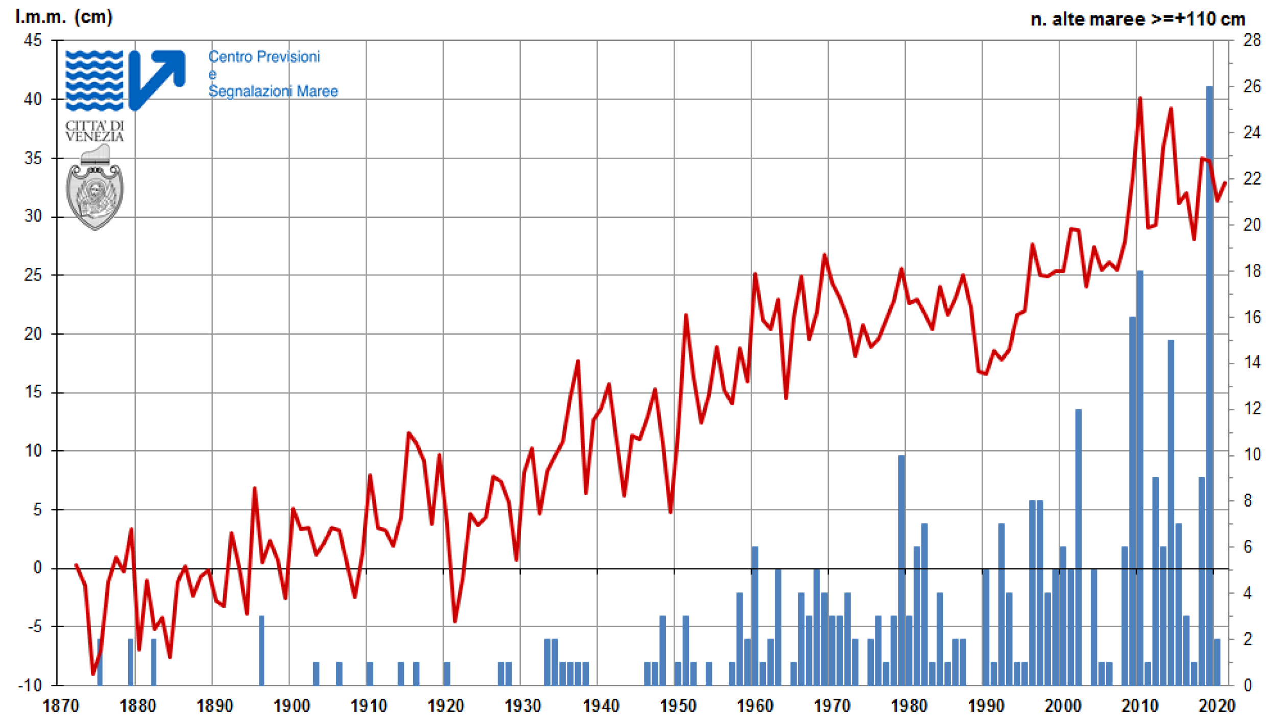
The meteorological condition responsible for the occurrence of the sirocco wind that produces storm surges in the Gulf of Venice is described in [1], among others. It is a deep low-pressure system that moves from west to east of the Adriatic basin, channeling the airflow along the Adriatic and making it interact with the high orography of the surrounding coastal regions, the Apennines to the west and the Dinaric Alps to the east. After the low-pressure system leaves the basin, bora often sets in, sometimes determining water level differences, between the southern and the northern sides of the Venice Lagoon, that may exceed 50 cm [2,3,4]. The complex interaction of the wind flow with the topography of the basin thus requires accurate wind field forecasts, which, on the other hand, often misrepresent the wind pattern observed by in-situ measurements and remotely sensed observations of satellite scatterometers. In the last 150 years, an evident positive trend has been registered in Venice for both the yearly number of high water events and the mean sea level height, as shown in Figure 2 (Courtesy of Centro Previsioni e Segnalazioni Maree, Comune di Venezia(Tide Forecast and Early Warning Centre of the Venice Municipality—CPSM) http://www.comune.venezia.it/it/content/variazioni-livello-medio-mare, accessed on 23 December 2022). The trend is likely to persist in the next decades [5]. The mobile barrier system MO.SE. (http://www.mosevenezia.eu/, accessed on 15 February 2023) has been realized, and has started to protect Venice and its lagoon from flooding since late 2020. Nonetheless, it is still necessary to predict and monitor the storm surges approaching the Gulf of Venice: the closing and opening of the mobile barriers have to be accurately managed to minimize the negative impact on the economic, health and emergency sectors and on the transport of people and goods.
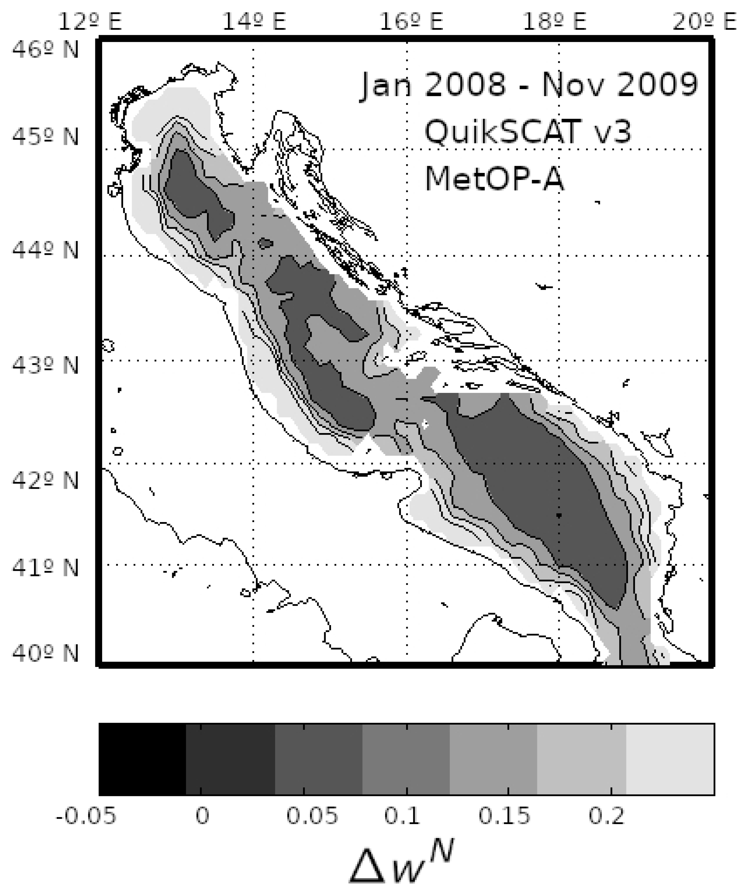
Storm surge models (SSMs) are routinely used to forecast the sea level in the Gulf of Venice and inside the Venice Lagoon. They rely on numerical weather prediction (NWP) model fields of wind and pressure as forcing inputs. The initial conditions of the surge at the beginning of the forecast simulation, namely the sea surface vertical displacement and the water transport zonal and meridional components, are also needed in order to perform realistic simulations of the surge. A relatively simple way to estimate the accuracy of the NWP model sea surface winds is to compare them with scatterometer observations. Satellite-borne scatterometers remotely sense the roughness of the sea surface, which is in equilibrium with the wind, and reveal the wind speed and direction by inversion of the radar backscatter values, using a geophysical model function (GMF) (see, for example, [6]). Scatterometer wind fields have uneven temporal sampling, but spatial extension comparable to that of NWP models. Often, they depict a different pattern of the sea surface wind with respect to NWP models. As an example, the representation of the statistics of the scatterometer-model wind speed bias, averaged over a period of almost two years (January 2008–November 2009), is reported in Figure 3: the relative bias between the European Centre for Medium-Range Weather Forecasts (ECMWF) analysis wind and the remotely sensed wind is always positive (ECMWF underestimates winds with respect to scatterometer), reaching 25% along the coasts [7].
Building on the assumption that scatterometers offer a more realistic representation of the wind field at the sea surface in coastal areas with complex orography, ref. [8] proposed a new methodology, called wind bias mitigation (WBM), for exploiting scatterometer observations to reduce the bias of numerical model wind field predictions with respect to satellite-detected winds. However, such methodology has a drawback, as it could lead to inconsistent results in some cases. The focus of this study is to reformulate the WBM methodology through a set of alternative candidate algorithms that avoid the weaknesses leading to incongruous consequences and to assess the performance of the candidates with respect to the original formulation.
The content of this study is structured as follows: the “Literary review” section gathers all the literature relevant to the contextualization of the research. In the following section, “Materials and Methods”, we describe the satellite and model data used in this study, and recall the original formulation of the methodology. The proposed improvements to the latter, which are the scientific focus of the research, are introduced immediately after through the characterization of the different alternative candidates to the original WBM algorithm. In the “Results” section, we present the statistical analysis, which we briefly discuss in the following “Discussion” section. The second last section is dedicated to the conclusions, while the future perspectives of this research are declared in the last section.

2. Literary Review

Previous works comparing scatterometer observations and NWP model forecasts were based on the analysis of a high number of observed and simulated collocated data. Ref. [9] compared QuikSCAT L2B 25 km observations and wind field forecasts produced by the Quadrics Bologna Limited-Area Model (QBOLAM) over the Mediterranean Sea. They found areas of lower-than-average forecast skill and identified these areas as being semi-enclosed basins surrounded by rough orography. Ref. [10] compared, on a monthly basis, the QuikSCAT 25 km data with “analysis quality” NWP winds (A. Wallcraft, personal communication, 2014) coming from the NOGAPS dataset at 0.5° of resolution in the Mediterranean Sea. Their findings confirmed that small basins surrounded by mountains are areas where the atmospheric modeling performance is lower than in the open ocean. The spatial and temporal structures of the monthly mean wind vorticity fields over the Mediterranean Basin, derived from satellite scatterometers and the ECMWF global atmospheric model winds, respectively, were investigated in [11]. They found a substantial similarity between the model and the scatterometer vorticity at spatial scales larger than 100 km, not confirmed at shorter scales in regions where the variability of the vorticity is influenced by the coastal orography. The mean relative bias and centered root mean square difference of scatterometer and model wind speed fields over the Mediterranean basin were analyzed in [12] and found dependent on the distance from the coast. The significant deviation from neutral values discussed therein was ascribed to the inadequate modeling of the wind flow interacting with the steep and high orography of the coastal regions. Even if scatterometer winds are operationally assimilated into the ECMWF global atmospheric model, it is commonly understood that assimilated winds do not reflect the surface wind patterns at spatial scales below a certain length. Indeed, the coarse spatial strategy (thinning) used in the assimilation process uses a single scatterometer observation (at 50 km spatial resolution) every 100 km [13]. Moreover, the spectral density of kinetic energy associated with the ECMWF model winds in the spatial mesoscale range is underestimated with respect to scatterometer observation [14]. These circumstances ensure that the independence of ECMWF winds from the assimilated scatterometer data, in the spatial mesoscale range can be taken as a reasonable assumption [8]. In the same study, the WBM methodology was delineated and proposed as an operational tool for reducing the bias between the model and scatterometer wind fields, especially in coastal areas. Refs. [7,15,16] take advantage of the methodology described in [8], adapting a combined strategy based on satellite scatterometry and satellite altimetry in order to improve the prediction skills of a hydrodynamic model used for storm surge forecast in the Adriatic Sea and Venice, with positive results. In their study, the surface wind field was provided by the ECMWF numerical atmospheric model, and scatterometer winds were derived from the SeaWinds scatterometer mounted on the American NASA QuikSCAT satellite and from the ASCAT instruments onboard the European MetOP satellites. Altimetry data were provided by the Center for Topographic Studies of the Ocean and Hydrosphere (CTOH) and assimilated in the numerical hydrodynamic model. Separate reanalysis for several historical Storm Surge Events (SEVs) in the Adriatic Sea was conducted using both scatterometer winds and altimetry sea level heights, then only one of the two, and finally without Earth Observation (EO) data (control runs). In almost all of the cases, the reanalysis experiments with EO data performed better than the control runs. Ref. [17] applied a technique similar to that described in [8] to improve the forecast of storm surges, and tested it in three hurricane events landfalling on the US coast. They used the analysis of wind fields produced by the Multi-Platform Tropical Cyclone Surface Wind Analysis (MTCSWA), developed by the National Hurricane Center (Florida, US), as forcing into a storm surge hydrodynamic model. The forcing winds were produced by multiplying the parametric wind field zonal and meridional components by a factor (innovation factor, IF) depending on the parametric and the analysis wind fields at the previous time step. Differently from the studies of the previous authors, that consider wind speed and direction separately, the formulation proposed in these three experiments acts on the zonal and meridional components independently. Apart from this aspect, the mathematical algorithm is analogous. The approaches proposed by [8,17] are similar and can be easily implemented, but little attention has been given, in our knowledge, to the mathematical derivation of the algorithm. In this study, we briefly revisit the bias reduction methodology in the original formulation of the algorithm, and then propose possible alternatives to it. We assess the performances of the original algorithm and of their alternatives, applying them to four datasets that can be seen to form the general phenomenology of storm surges in the northern Adriatic Sea.
The quality of the NWP wind forcing has a direct impact on the accuracy of the modeled surge, as forcing input errors are propagated by the SSM and amplified by the inherent approximations in the SSM formulation and in the hydrodynamic initial and boundary conditions. It is thus essential to supply to the SSMs forcing inputs as close as possible to the real meteorological situation. As diffuse and accurate observations of the sea surface wind are possible today with satellite-borne scatterometers, it is worthwhile to assess a methodology able to exploit satellite wind observations for storm surge modeling purposes. An important achievement of the eSurge-Venice project, funded by the European Space Agency, was the development of the WBM procedure from its initial form to an operational tool. Indeed, the WBM procedure has proven to be able to reduce the model-scatterometer wind bias and improve the performance of a storm surge model [7,15,16]. Regardless of the specific context of sea level forecasts, the WBM process was first introduced in [8], where the performance of WBM was assessed for a dataset consisting of thirty-three cases of high water in Venice in the period 2004–2014. These cases were selected as occurring at the same time as significant storm surges observed in the Gulf of Venice. The assessment regarded the improvements brought by scatterometer observations through the WBM procedure to the sea surface wind forecasts provided by the ECMWF global atmospheric model. In these experiments, the WBM methodology relied on a simple yet effective algorithm to tune the model wind according to its bias with the scatterometer. In [8], as well as in the present study, the hypothesis is that the wind speed derived from the scatterometer observations is the ground truth, while the model wind speed is an estimate that can be improved in order to give a more accurate description of the wind field at the sea surface. As the WBM methodology has reached a decent level of maturity, we decided to extend the WBM approach to different datasets, introducing alternative mathematical formulations of WBM in order to reduce the limitations of its original expression and to assess their performances. The most appropriate among the candidates has been used in the sea-level forecast chain of the Tide Forecast and Early Warning Centre of the Venice Municipality Centro Previsioni e Segnalazioni Maree, Comune di Venezia—CPSM), Venice’s local public agency in charge of issuing tide forecasts.

3. Materials and Methods

3.1. Materials: Model Wind

In this work, we have used the surface wind fields produced by the medium-range, high-resolution (HRES) global deterministic model of the ECMWF Integrated Forecasting System (IFS) at the original resolutions and at synoptic hours, interpolated on a regular grid with 1/8th of a degree pass. The zonal and meridional components of the wind field are given at 10 m height from the surface. The local stability conditions of the air–sea interface are accounted for in the model. The forecast winds used are those for which the valid time is within twenty-four hours of the base time.

3.2. Materials: Scatterometer Wind

In our study, we have used the scatterometer ocean wind vector (OWV) of the NASA QuikSCAT satellite, the EUMETSAT MetOp-A and MetOp-B satellites, and the ISRO Oceansat-2 satellite. For QuikSCAT, the product used is the L2B version 3 (1999–2009) [18]. For MetOp the wind products are multiples: ASCAT-A L2 (2007–2015), ASCAT-A L2 Coastal (2010–present), and ASCAT-A/B L2 Coastal (2010–2021 and 2012–present, respectively) [19]. The ASCAT “coastal” L2B dataset differs from the standard ASCAT L2B dataset as the σ 0 retrievals are filtered with a spatial box instead of a Hamming window so that all the sea data within a 15 km radius of the centroid of the cell contribute to its value, while non-sea retrievals are discarded. After the inversion of σ 0 , winds can be computed up to 15 km from the coast instead of the standard product (non-coastal) that is cut off at 35 km from the coast. For Oceansat-2, the product used is the L2B (2010–2014) [20]. All the scatterometer winds are given at the nominal resolution of 12.5 km. QuikSCAT and Oceansat-2 winds have a minimum distance of 20 km from the coast. The scatterometer ocean wind vector is calculated in equivalent neutral atmospheric conditions. Thus, the scatterometer neutral winds have been corrected for the effects of atmospheric stability, using a boundary layer model [21] as described in [11]. Scatterometers use different sensors, radiation wavelength and observation geometry to measure the sea surface roughness from which the wind is determined by inversion through the GMF. Scatterometer wind data are also distributed by different agencies and research groups using different GMFs. Large biases have been evidenced between disparate sources of sea surface winds (modeled, remotely sensed and observed from various platforms). For example, [22] found that modeled winds can have biases up to several meters per second in strong winds and that observations can differ by similar quantities for winds as strong as 20 ms 1 . However, in the Adriatic Sea, wind speeds > 20 ms 1 are rarely observed [8,23]. Moreover, our study is focused on winds ranging from 10 to 20 ms 1 , as they matter most when storm surges are concerned in this region. In such a range, wind speed differences between the various sensors are within 1–2 ms 1 [22], and they should be negligible in the context of this study. The GMFs that originated the winds in our research are: for QuikSCAT and Oceansat-2 L2B, the Ku2011 GMF of the Remote Sensing System (RSS) [24]; for ASCAT, the CMOD5.n GMF [25]. The scatterometer data were finally interpolated on the same 0.125° regular grid used for ECMWF data, with a Laplacian method, which preserves the statistics of the original wind speed and direction dataset [9].

3.3. Methods: The Wind Bias Mitigation Procedure

The focus of our study is to retrace why and how the WBM procedure, a tool to improve the accuracy of the wind field forecasts introduced in [8], has been designed, as well as the reason why the original formulation could fail to give an acceptable solution in some particular conditions. To outflank such possibilities, alternative formulations are proposed and assessed in order to identify the most suitable for storm surge modeling purposes. As our objectives are operational SSM applications in the Gulf of Venice, we focus on this geographic area. Here, the ECMWF global atmospheric model supplies very high-quality forecast and analysis of sea surface wind fields, which, however, are generally underestimated: ref. [12] have found that scatterometer-model wind biases in the Mediterranean Sea are variable in space and time and increase toward the coast. Refs. [9,11,12] investigated the affinities and disagreements of scatterometer wind observations and their replication given by numerical models by means of the relative wind speed bias δ w N ( i , j , t ) , defined as:
δ w N ( i , j , t ) = w s ( i , j , t ) w m ( i , j , t ) w s ( i , j , t )
where w ( i , j , t ) is the considered quantity (scatterometer or model wind speed) at the grid node ( i , j ) and time t. In our study, we adopt the same 0.125° × 0.125° regular grid on which both scatterometer and model winds are reprojected. The superscript “s” and “m” refer to the scatterometer and model, respectively. The difference in the two wind speeds is taken with respect to the scatterometer wind, which is expected to better represent the meso- and submesoscale variability in coastal zones where the orography contributes to the shape of airflow [9].
Averaging Δ w N over a given period at each node of the grid permits obtaining statistically reliable estimates of the relative wind speed bias:
Δ w N ( i , j ) = w s ( i , j ) w m ( i , j ) w s ( i , j ) = 1 N k = 1 N w k s ( i , j ) w k m ( i , j ) w k s ( i , j )
where the temporal average is represented as the sum over N time steps t 1 , t 2 , . . . , t k , . . . , t N , and the dependence on time has been substituted by the discrete index “k”.
The average number of scatterometer passes over the Adriatic Sea is around 3–4 times a day, with maxima during limited periods of simultaneous operations of QuikSCAT/MetOP-A and Oceansat-2/MetOP-A and -B (4–6 passes a day). With such a low number of collocated scatterometer-model data at each grid point, it is necessary to collect and average scatterometer observations during a period of some days in order to obtain statistically reliable quantities. However, arbitrarily enlarging the averaging window would turn to a loss in correlation between observations pertaining to different meteorological patterns, thus reducing their statistical significance. For the present application, the optimal size of the averaging period resulted in three days [8].
The scatterometer model’s relative bias, calculated in Equation (2), comes in handy for performing a tuning of the NWP wind field in order to reduce the model bias with respect to the remotely sensed wind. Such a procedure, which we call wind bias mitigation, has been investigated from the perspective of storm surge forecasting by [8]. In such a study, the relative wind speed bias Δ w N ( i , j ) was used as a counteracting term in order to nudge the model output toward the satellite retrievals, i.e.,
w m ( i , j ) = w m ( i , j ) 1 + Δ w N ( i , j )
In Equation (3) the primed quantities represent the model winds after the application of the bias mitigation procedure, while the quantity 1 + Δ w N is called the bias mitigation factor (BMF).
The relative wind speed bias, determined by the running averaging window of three days, is used to tune the model wind fields of the day after the end of the averaging window. The process is replicated for all of the days in the period under study until a time series of wind bias mitigation factor daily maps covering that period is generated.
In our study, the surge events (SEVs, or "cases") are defined as a sequence of three days: for each of these three days (say d 1 , d 2 and d 3 ), a single wind bias mitigation map is formed, accounting for the relative bias between the collocated model analysis and scatterometer wind retrievals of the three days preceding each of them, as described by Equation (2): (d 2 ,d 1 , d 0 ) for d 1 . Analogously for d 2 (d 1 ,d 0 , d 1 ) and d 3 (d 0 ,d 1 , d 2 ). Then, the bias-mitigation map is used to mitigate the bias of the model forecast wind speed of days d 1 , d 2 and d 3 separately, as prescribed by Equation (3). Finally, the three days d 1 , d 2 and d 3 are considered together, and statistical analysis of the bias-mitigated model forecast, the original model forecast and the scatterometer observations are performed.

3.4. Methods: Original and Alternative Mathematical Approaches for the Calculation of the Bias Mitigation Factor

The original formulation of the model wind speed correction factor ( 1 + Δ w N ) in Equation (3) [8], henceforth indicated as “Original Formulation” (OF)), was developed heuristically. As a consequence, its definition is weak, as it could occasionally also take negative values. Omitting the spatial indexes ( i , j ) in the following discussion, we have:
1 + Δ w O F N = 1 + w s w m w s = 1 + 1 N k = 1 N w k s w k m w k s = 2 1 N k = 1 N w k m w k s
When k = 1 N w s ( t k ) m o d e l w s ( t k ) s c a t t > 2 N the factor ( 1 + Δ w N ) in Equation (4) is oddly defined, as it becomes negative and determines negative values of the model wind speed when used in Equation (3). Indeed, for a small number of collocated model and scatterometer observations at the same location ( i , j ) , and/or for small wind speeds and/or particularly unfortunate predictions, or when the meteorological conditions change drastically during the same SEV in a short period of time, it is not unlikely that many or all of the terms in the sum k = 1 N w s ( t k ) m o d e l w s ( t k ) s c a t t are greater than two, so that they add-up to something > 2 N . A partial solution to this problem is to perform the mitigation process based on thresholds that can be adapted easily in order to prevent such a situation. Nonetheless, as we will see, Equation (3) works rather well, putting a lower threshold of 0 to the values in the bias-mitigation maps.
In our opinion, however, it is more desirable to formulate alternative and well-defined algorithms in order to obtain consistently defined mitigation factors (MF). This led us to consider alternative mathematical definitions for the WBM procedure, which can ensure analytical consistency in the algorithm. They are:
  • AF1 and AF2—surrogates of the original algorithm: based on the definition of the OF, but with a regularized denominator, preventing the anomalous behavior of OF when k = 1 N w s ( t k ) m o d e l w s ( t k ) s c a t t > 2 . AF1, the first surrogate, uses the model wind speed instead of the scatterometer wind speed as the denominator in Equation (5), while the denominator of the second (AF2) is the mean value of the scatterometer and model wind speed (Equation (6)):
    1 + Δ w A F 1 N = 1 + w s w m w m
    1 + Δ w A F 2 N = 1 + w s w m 1 2 ( w s c + w m )
    In AF1, the wind speed increment is relative to the model wind instead to the scatterometer wind. This choice entails a better definition than OF, as 1 + Δ w A F 1 N = 1 N k = 1 N w k s w s k m , i.e., it is positively defined unless some of the model wind speeds are equal to zero.
    In AF2, the increment in wind speed is relative to the average of the two wind speeds at each step t k . As one can easily see, in such case the mitigation factor 1 + Δ w A F 1 N is equal to 2 N k = 1 N w k s w k ¯ , where w k ¯ = w k s + w k m 2 , and the result is always 0 and well-defined unless at least one of the w k ¯ is zero;
  • Analytical solution (AS): It is determined from the definition of bias-mitigated model wind (Equation (3)):
    w k m = w k m 1 + Δ w N ,
    and constraining to zero the relative difference between the scatterometer and the mitigated model wind (primed quantities are the mitigated ones):
    w s w m w s = 1 w m w s = 0 .
    Substituting the expression of Equation (3) for w m in Equation (7), we have:
    k = 1 N w k s 1 + Δ w N w k m w k s = N 1 + Δ w N k = 1 N w k m w k s = 0
    and thus:
    1 + Δ w A S N = 1 N k = 1 N w k m w k s 1
  • Least square regression approach: A vast class of optimal solutions to the bias-mitigation procedure comes from the least square regression approach (LSR). In the following, we consider two classes of solutions; the first is “linear”, the second is “relative”, obtained by minimizing specific functions of the residuals, which depend on the wind speed of the scatterometer and model, and parameter α :
    δ α = f ( w k s , w k m , α ) δ α α = 0
    -
    Least square regression of linear type (LLSR and LLSR E ): a LSR of linear form is used in the minimization of the sum of the squared residuals of the differenced scatterometer minus model determinations, with respect to parameter α , which corresponds to Δ w N to be determined.
    The first approach considered in this study is the simplest: the function to be minimized is the squared sum of the residuals formed by the scatterometer and the bias-mitigated model wind speeds. Parameter α is hidden in the definition of the latter:
    δ α = k = 1 N w k s w k m 2 = k = 1 N w k s ( 1 + α ) w k m 2
    the solution, in this case, is given by:
    1 + Δ w L L S R N = k = 1 N w k m w k s k = 1 N ( w k m ) 2
    The second of the linear LSR approaches (LLSR E ) takes into consideration the dependence of the sea surface wind stress on the squared wind speed [26], as well as the dependence of the surge level on the squared wind speed in theoretical [26] and empirical [27] models. This requirement is formalized in the formula by inserting the squared instead of the linear wind speeds:
    δ α = k = 1 N ( w k s ) 2 ( w k m ) 2 2 = k = 1 N ( w k s ) 2 ( 1 + α ) 2 ( w k m ) 2 2
    and the solution is:
    1 + Δ w L L S R E N = k = 1 N ( w k m ) 2 ( w k s ) 2 k = 1 N ( w k m ) 4 1 2
    -
    Least square regression of relative form (RLSR and RLSR E ): it has been suggested that, in cases where relative variations are more significant than absolute variations, a relative form of LSR is more suitable then a direct one [28]. This indication perfectly fits the problem we are facing in our study. Even in the Relative LSR we adopted two minimization approaches: in the first (RLSR), the minimization is performed on the sum of the squared residuals, weighted by the inverse of the scatterometer wind speed:
    δ α = k = 1 N w k s w k m w k s 2 = k = 1 N w k s ( 1 + α ) w k m w k s 2
    with solution:
    1 + Δ w R L S R N = k = 1 N w k m w k s k = 1 N w k m w k s 2
    In the second formulation (RLSR E ), the wind speeds in the numerator appear squared, while the weights are the same as in the linear case:
    δ α = k = 1 N ( w k s ) 2 ( w k m ) 2 w k s 2 = k = 1 N ( w k s ) 2 ( 1 + α ) w k m 2 w k s 2
    with solution:
    1 + Δ w R L S R E N = k = 1 N ( w k m ) 2 k = 1 N ( w k m ) 4 ( w k s ) 2 1 2
In some cases, the algorithms of the WBM give wind speeds beyond the physical limits found in the Mediterranean Sea. To avoid such unrealistic values of the mitigated wind speeds, we apply two sets of thresholds: the first filters out insufficient or excessive values of the MFs, setting each MF value outside the interval [0.9 1.2] to the nearest of the two limits: 58% of the MF values are in this range. The second set of thresholds acts on the wind speeds, limiting too low or too high winds in input and output. The thresholds are: for scatterometer wind speed, a minimum of 3 and maximum of 33 ms 1 ; the minimum number of observations per grid point is 4; for model wind speed, the minimum is 0 and the maximum is 33 ms 1 .

3.5. Methods: Statistical Analysis and Parameters Used in the Comparison

The performance of the WBM procedure is assessed by comparing mitigated and non-mitigated forecast wind speeds against the scatterometer-collocated ones, which in our analysis, represent the ground truth. It is important to underline that we compare (modified) model wind fields against scatterometer wind fields, and the statistical analysis is based exclusively on such comparison: we do not take into consideration observed or expected surge levels in the assessment but only scatterometer and NWP forecast winds.
The statistical analysis has been conducted on four different datasets:
  • D1: a historical dataset of 29 Storm Surge Events (SEVs) occurred between 2004 and 2014 in the Adriatic Sea, which triggered high water in the Venice lagoon, with an observed surge of >40 cm. This dataset has been considered here as it was first used by [8] and thus represents a natural test bed for the alternative mathematical approaches that we will introduce later. In our processing, the overlapping SEVs in D1 have been removed;
  • D2: a second dataset has been arranged to integrate D1 with more recent SEVs, for a total of 48 cases (observed surge > 40 cm) between 2013 and 2016. In such a period, Venice experienced an unusually high number of high waters. Note that, while in 2004–2014, we count 29 SEVs, i.e., 2.6 SEV per year, in 2013–2016, this figure has risen to 12.0 SEV per year;
  • D3: the third dataset is formed by 364 cases of random sea level conditions in the same years as the second (2013–2016) and has been included to test the wind bias mitigation procedure in operational-like conditions, to assess the behavior of the WBM procedure with respect to false positivity. Cases are picked up once every four days so that wind conditions are random and completely unrelated to storm surge occurrence;
  • D4: the fourth is formed by the seven SEVs, between 2012 and 2016, the worst predicted by the Tide Forecast and Early Warning Centre of the Venice Municipality (A. Tosoni, 2017—personal communication).
For the comparison, the following statistical parameters have been used:
  • centered root mean square difference (cRMSD): the cRMSD is the root mean square difference (RMSD) of two series after removing their means;
  • standard deviation: standard deviation of each series;
  • Person’s linear correlation coefficient: linear correlation of two series;
  • bias: difference of the mean values of two series;
  • success rate (SR): in this context, it is the percentage of times in which the SEV averages of the mitigated model winds were closer to that of the observed winds compared to the average of the non-mitigated model winds;

4. Results

To exemplify how the wind bias mitigation changes the model winds with respect to the scatterometer retrievals and the standard model forecast, in Figure 4, we report the distribution of the wind speed of the scatterometer, standard forecast and the eight mitigated model forecasts, as they are defined by the mitigation procedure and by the eight different formulations of the mitigation factor, for the SEVs of dataset D4. The black solid line is the distribution of all the scatterometer winds that fall into the D4 dataset. The black dash-dotted line represents the distribution of the standard forecast wind speed. The original formulation is plotted as the purple dotted line with diamond markers. The winds related to the seven new formulations of the MF are plotted in other colors as per the legend. The underestimation of the standard forecast with regard to the scatterometer winds is evidenced by the drop in the forecast distribution at ∼12 ms 1 with respect to the black solid line. The mitigated forecasts compensate for the drop in the standard forecast in the region 11−20 ms 1 . They follow the troughs and crests of the scatterometer line, even if they underestimate the scatterometer wind in the region 3−11 ms 1 . However, in this region, the winds are feeble, and possible biases weigh less than in the region of stronger winds. As we omit scatterometer winds below 3 ms 1 , in the range 0−3 ms 1 , mitigated and non-mitigated winds are overlayed.
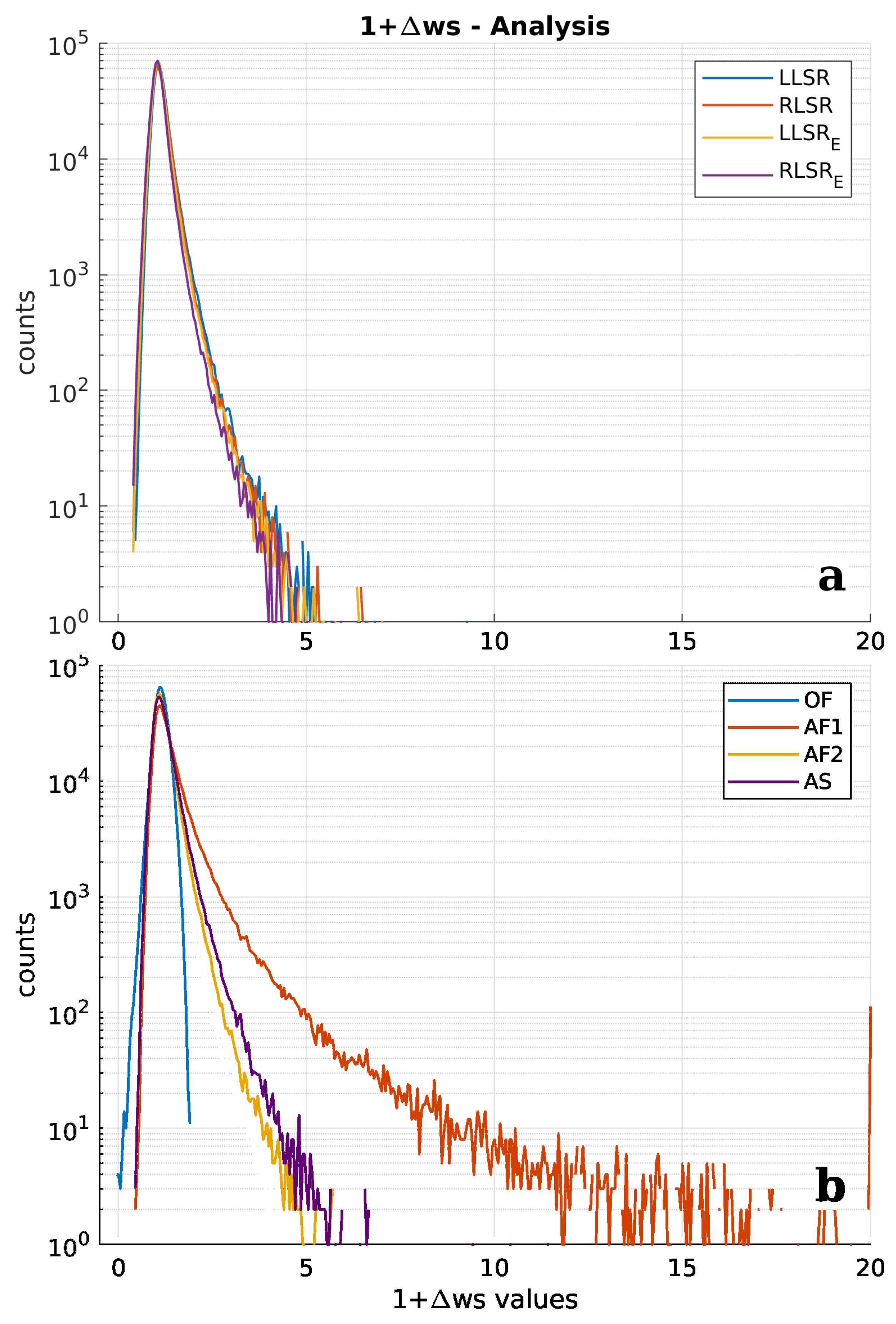
The probability distribution of the MFs ( 1 + Δ w N ) for the D3 dataset, as an example, is depicted in Figure 5: on the upper panel, the distributions of the MF for the LSR methods are reported, while the bottom panel shows the MFs of the other four methods (OF, AF1, AF2 and AS), all in a log scale on the y-axis. The values shown here have not yet been thresholded to facilitate discussion. The anomalous behavior of the OF MF distribution is evidenced by the plots of the right panel of the figure: it allows negative values, and exhibits a characteristic profile, different from the other MFs, falling down to zero at (near) 2: this value is derived directly from Equation (4), when all the w k m are equal to zero. All the other MF distributions do not take negative values and extend toward much higher values on the positive side of the x-axis.
The statistical summary reported in Table 1 shows that the distribution of the OF MF is the only one with negative skewness. It is also the one that most follows a normal distribution (skewness −0.01, kurtosis 3.71). The probability distribution of all the other MFs have positive and higher skewness and much higher kurtosis. This is particularly the case for the distribution of the AF1 MF, which, having the model wind speed as the denominator in the MF expression (Equation (5)), evidences how the model wind is often underestimated with respect to the scatterometer wind and results in having the longest and most populated right side tail among all the MFs, as demonstrated by its highest skewness, kurtosis and standard deviation.
We now consider Taylor’s diagram [29] relative to the D3 dataset, which had the worst performance among the four datasets considered, as an example. Taylor’s diagram allows a synoptic view of three statistical estimators: the standard deviation, the centered root mean square difference (cRMSD) and Pearson’s linear correlation coefficient of a set of experimental data with respect to a reference. In our context, the scatterometer is taken as a reference, while the non-mitigated and the mitigated model wind speeds form the data set to be assessed. The position of the mitigated forecast values for the eight different WBM approaches, in terms of cRMSD, linear correlation coefficient and standard deviation, are found in Taylor’s diagram of Figure 6, not far from the unmodified forecast. The non-mitigated and mitigated forecast indicators are colored according to their bias with respect to the scatterometer observations: the non-mitigated ones are yellowish, while the mitigated ones are blue to green. The color bar on the diagram’s side reports the mapping between the bias color and its value. Figure 6 shows the values of the four statistical indicators considering all the collocated model-scatterometer pairs, independent of scatterometer pass or SEV. Original and mitigated forecasts have very similar statistics in terms of standard deviation, cRMSD and linear correlation: they are aligned very close in the diagram, indicating that the statistical properties of the mitigated winds are conserved, whichever algorithm is considered. However, it strongly affected the fourth estimator, the wind speed bias of the mitigated forecasts with respect to the non-mitigated one. The lower value of the bias of the mitigated forecasts with respect to the non-mitigated model wind is a good indication that the WBM methodology effectively nudges the model wind closer to the observations. While the biases remain substantially similar, whether the statistics are calculated on the series of individual pairs or the pairs are grouped by SEV beforehand, the other three statistical indicators, namely cRMSD, correlation and standard deviation, improve when calculated as the averages of each SEV. This detail is encouraging because the effect of the wind on the surge depends on the average over large regions rather than on particular local behaviors.
Table 2 (fourth row for the D3 dataset) reports the biases between the scatterometer set of observations and the corresponding set of the standard forecast in the third column, and from the fourth to the eleventh columns, reports the bias between the scatterometer and the eight mitigated forecast solutions. For all the datasets, the bias of the standard forecast with respect to scatterometer observations ranges from 0.84 ms 1 , while for the mitigated forecasts, its maximum value is 0.46 ms 1 (minimum −0.50 ms 1 ). In general, the mitigated forecasts have lower bias, in modulus, than the standard forecast.
The results for the RMSD of the mean wind speed of the scatterometer and original forecast, and of the scatterometer and the eight different formulations of the mitigated forecasts, grouped in SEVs, are reported in Table 3. All the RMSD of the mitigated forecast winds are lower in all eight different flavors of the mitigation, with respect to the original forecasts, for all four datasets. It could seem that such a lower difference in the mean wind speed values between mitigated and non-mitigated model winds has a small relevance. Actually, for storm surge modeling applications, the prominent quantity is the wind stress, which is proportional to the square of the wind speed: the relative change in the drag exerted by the wind on the sea surface is twice as large as the relative bias of the wind speed that caused it. Thus, even a small reduction in the wind speed bias between the model and observations brings significant improvements, especially when the NWP data are employed to force hydrodynamic applications through the wind stress drag on the sea surface [30].
Table 4 reports the success rate for the four datasets and the eight mitigation flavors. It is worth noting that the mitigated winds have a success rate ranging from 70% to 100% (mean SR: 76%). Among them, the LLSR E WBM approach has the highest score in all datasets.
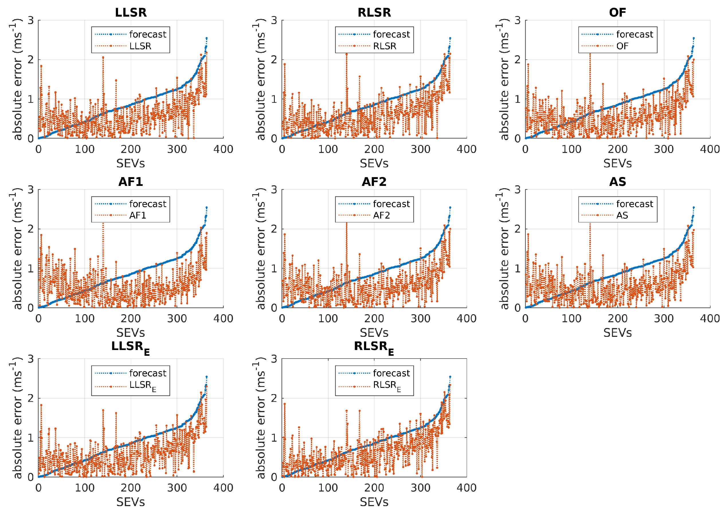
The numbers reported in Table 4 for the D3 dataset are derived from the data plotted in Figure 7.
Here, the absolute error of the mean mitigated forecast and the scatterometer winds for each SEV of dataset D3, are plotted in orange and ordered by increasing the absolute error of the mean standard forecast and the scatterometer winds. The latter are reported in blue (they are the same in all eight plots). In practice, SR is the number of orange markers above the blue markers divided by the total number of SEVs, multiplied by one hundred. Very small differences are seen from plot to plot, and the SR of the LLSR E MF is the same as the OF, AF2 and AS. However, the LLSR E approach performs best in all four datasets, indicating the superior overall performance of this MF over the others. Another feature of the LLSE E and RLSR E MFs is that both show lower absolute errors with respect to the other MFs where the standard forecast absolute error is low (first 100 or so). On the other hand, AF1 performs better for the SEVs from 200 up to 364.

5. Discussion

In the previous section, we have reported the results of the bias mitigation procedure, realized by using eight different mathematical formulations of the mitigation factor, expressed by three different statistical indicators: bias, RMSD and SR. Finally, we report here two tables, summarizing the results for the most significant statistical indicators, which are bias and SR, as the RMSD and Pearson’s linear correlation coefficient does not change significantly across the four datasets and the eight mitigation approaches.
In Table 5, we report the bias and FR averaged over the four datasets (by column), where the averages are weighted by the number of cases in each dataset. Table 6 is very similar to the previous one, with the exception that the datasets considered are D1, D2 and D4 only, i.e., the datasets populated with only real SEV events: D3 dataset is omitted as it does not contain real SEVs, contrary to the other three. In each row of the two tables, we have marked the two best results of the row in bold to facilitate the verification of the mitigation factor that gave the best performance.
The weighted averages used to calculate the two indicators in Table 5 and Table 6 present the performance more accurately, as the results of the statistical indicators have been weighted by the number of events populating each individual dataset. Indeed, the number of events varies dramatically across the four datasets. Moreover, Table 5 is suitable for representing the best mitigation approach for generic situations in which real storm surge events (strong wind) alternate with weak wind events. On the contrary, Table 6, considering only the three datasets formed by real storm surge events, evidences the mitigation approach preferred in the case of strong winds. In the first case (balanced occurrence of strong and weak wind), two mitigation approaches perform better than the others: AS and LLSR E ; in the second (strong wind and thus optimized for storm surges), four approaches perform almost equally well: LLSR E , AF2, AS and LLSR. Thus, LLSR E and AS resulted in the best-performing and most versatile mitigation approaches. Of the two, LLSR E is preferred when the success rate is critical.

6. Conclusions

In this study, we have analyzed the structural and statistical aspects of a method designed to reduce the bias between the sea surface wind observed by the scatterometers and that forecasted by a state-of-the-art numerical model in coastal regions. The method, called “bias mitigation”, exploits scatterometer observations of the sea surface wind to determine a correction factor ( 1 + Δ w N ) to modulate the standard model wind as w m o d e l = w m o d e l ( 1 + Δ w N ) and to nudge the wind forecast closer to observations. We compared eight different mathematical formulations for deriving the factor Δ w N , and assessed these eight formulations over four datasets (D1–D4), using five statistical parameters: cRMSD, Pearson’s linear correlation coefficient, standard deviation, bias and success rate. We found that the standard forecast and the eight mitigated forecasts have similar centered CRMSD (scatt-model), comparable Pearson’s linear correlation coefficient and similar standard deviation. However, the mitigated forecasts have, in general, a significantly smaller bias, with respect to the scatterometer observations, than the standard forecast. The cRMSD, Pearson’s correlation coefficient and the standard deviation are almost constant across the four datasets and the eight mitigation methods, evidencing low sensitivity in this respect. For this reason, the final conclusions are based mostly on the bias and the success rate statistical parameters. The biases of the eight mitigated forecasts range between −0.50 and 0.46 ms 1 (Table 2), and are always lower than the standard forecast, which results in the underestimation of the scatterometer observations by 0.84 to 0.97 ms 1 (dataset averages, Table 2). The success rate of the mitigated forecasts also remains high (>70%) across the four different datasets and the eight mitigation factors. More accurate wind forecasts mean better prediction of the surge levels: a circumstance of the utmost importance for the delicate equilibrium in which water and land coexist along the coast of the Gulf of Venice and the Venice Lagoon. Here, daily life depends on the correct prediction of the high waters, even now that the MO.SE. barriers have been put into operation. Among the eight formulations of the mitigation factor considered, AS and LLSR E have similar performances, while the other formulations (OF, AF1, AF2, LLSR, RLSR and RLSR E ) performed slightly worse, still getting closer to remotely sensed winds than the non-mitigated forecasts. As seen in Table 5, LLSR E does not lower the bias with respect to the original formulation, OF (0.31 vs. 0.16 ms 1 ), while AS does (0.10 vs. 0.16 ms 1 ). In our opinion, such small differences in bias between the MFs are not significant. The success rate of these three MFs (OF, AS and LLSR E ) are also the same (Table 5). When the success rate is critical, however, we believe that the LLSR E approach should be preferred over the others: the biases of the three MFs (OF, AS and LLSR E ) are 0.05, −0.02 and 0.40 ms 1 , respectively, while the success rates are 73.74, 76.26 and 81.89. For LLSR E , the relative increment in success rate with respect to OF is 11% ( S R L L S R E S R O F S R O F ). A similar performance is reached by LLSR. The analysis shows a misleading result about biases: they are small, with no or little improvement with respect to OF. However, the overall bias is not the whole story, as every SEV has a different distribution of the wind, and a MF can have a success rate notably higher than another even if their overall biases are similar. In our analysis, the wind bias mitigation procedure brings clear advantages when storm surges are favored by meteorological conditions. Likewise, the mitigation procedure is also effective in standard or non-critical meteorological conditions, even with slightly worse performances. For these reasons, CPSM has adopted the mitigation procedure in the LLSR E formulation for the operational storm surge prevision chain, where timeliness is critical: scatterometer observation sare acquired with a ∼3 h latency, while ECMWF model fields are received twice a day with higher latency (∼7 h).

7. Perspectives

The wind direction bias has been partially considered in [7,15] using a single algorithm for the derivation of the mitigation strategy. Further investigations are ongoing about the possibility of using circular statistics strategies to obtain statistical estimators of the wind direction bias, using, for example, the methods discussed in [31,32]. The absence of a suitable mechanism to take into account the effects of the wind direction on the representation of the surface wind field is clearly an issue in the present formulation of bias mitigation. For this reason, the impact of wind direction bias correction schemes will be analyzed and presented in a future study. Likewise, the performances of the bias mitigation method need to be assessed in a wider geographical context: a challenging task to be addressed with limited resources. On the other hand, the reasons for the residual failures of the WBM scheme have not yet been addressed but deserve full attention and will be faced soon. Finally, the impact of the mitigation strategy on the operational storm surge prevision made at CPSM, the only direct and straightforward way to assess the effectiveness of the WBM procedure, will soon be investigated.

Author Contributions

Conceptualization, F.D.B. and S.Z.; methodology, F.D.B.; software, F.D.B.; validation, F.D.B.; formal analysis, F.D.B.; investigation, F.D.B.; resources, F.D.B.; data curation, F.D.B. and S.Z.; writing—original draft preparation, F.D.B.; writing—review and editing, F.D.B. and S.Z.; visualization, F.D.B.; supervision, F.D.B.; project administration, F.D.B.; funding acquisition, S.Z. All authors have read and agreed to the published version of the manuscript.

Funding

This work has been partially supported by the European Space Agency (ESA) in the framework of the project Storm Surge for Venice (eSurge-Venice, http://due.esrin.esa.int/page_user472.php, accessed 23 December 2022) as part of its Data User Element (DUE) programme, contract number 4000104485/11/I-LG. It has been also partially supported by the Flagship Project RITMARE (https://maritime-spatial-planning.ec.europa.eu/projects/la-ricerca-italiana-il-mare, accessed 23 December 2022) funded by the Italian Ministry of University and Research.

Data Availability Statement

The satellite winds have been downloaded from the NASA Physical Oceanography Distributed Active Archive Center (PO.DAAC) at the Jet Propulsion Laboratory/California Institute of Technology (http://podaac.jpl.nasa.gov/, accessed 15 January 2017). The NWP model fields have been obtained from ECMWF thanks to the authorization from the Aereonautica Militare Italiana.

Acknowledgments

The QuikSCAT and Oceansat-2 winds have been processed by the Jet Propulsion Laboratory/California Institute of Technology; the ASCAT winds by the EUMETSAT Ocean and Sea Ice Satellite Application Facility (OSI-SAF). This study has been conducted in the framework of the Technical and Scientific Collaboration Agreement between the Institute of Polar Sciences of the National Research Council of Italy and the Tide Forecast and Early Warning Centre of the Venice Municipality. All images in this document except the image in Figure 1 have been made with MathWorks MATLAB© software, versions R2022a and R2022b. We kindly thanks MDPI for the economic support in publishing this research.

Conflicts of Interest

The authors declare no conflict of interest. The funders had no role in the design of the study; in the collection, analyses, or interpretation of data; in the writing of the manuscript; or in the decision to publish the results.

References

  1. Lionello, P.; Cavaleri, L.; Nissen, K.; Pino, C.; Raicich, F.; Ulbrich, U. Severe marine storms in the Northern Adriatic: Characteristics and trends. Phys. Chem. Earth Parts A/B/C 2012, 40–41, 93–105. [Google Scholar] [CrossRef]
  2. Zecchetto, S.; Umgiesser, G.; Brocchini, M. Hindcast of a storm surge induced by local real wind fields in the Venice Lagoon. Cont. Shelf Res. 1997, 17, 1513–1538. [Google Scholar] [CrossRef]
  3. Mel, R.; Carniello, L.; D’Alpaos, L. Addressing the effect of the Mo.S.E. barriers closure on wind setup within the Venice lagoon. Estuarine, Coast. Shelf Sci. 2019, 225, 106249. [Google Scholar] [CrossRef]
  4. Lionello, P.; Barriopedro, D.; Ferrarin, C.; Nicholls, R.J.; Orlić, M.; Raicich, F.; Reale, M.; Umgiesser, G.; Vousdoukas, M.; Zanchettin, D. Extreme floods of Venice: Characteristics, dynamics, past and future evolution. Nat. Hazards Earth Syst. Sci. 2021, 21, 2705–2731. [Google Scholar] [CrossRef]
  5. Church, J.A.; Clark, P.U.; Cazenave, A.; Gregory, J.M.; Jevrejeva, S.; Levermann, A.; Merrifield, M.A.; Milne, G.A.; Nerem, R.S.; Nunn, P.D.; et al. Sea Level Change. In Climate Change 2013: The Physical Science Basis. Contribution of Working Group I to the Fifth Assessment Report of the Intergovernmental Panel on Climate Change; Stocker, T.F., Qin, D., Plattner, G.K., Tignor, M., Allen, S.K., Boschung, J., Nauels, A., Xia, Y., Bex, V., Midgley, P.M., Eds.; Cambridge University Press: Cambridge, UK; New York, NY, USA, 2013; Chapter 13; pp. 1137–1216. [Google Scholar]
  6. Verspeek, J.; Stoffelen, A.; Portabella, M.; Bonekamp, H.; Anderson, C.; Saldana, J.F. Validation and Calibration of ASCAT Using CMOD5.n. IEEE Trans. Geosci. Remote Sens. 2010, 48, 386–395. [Google Scholar] [CrossRef]
  7. De Biasio, F.; Vignudelli, S.; della Valle, A.; Umgiesser, G.; Bajo, M.; Zecchetto, S. Exploiting the potential of satellite microwave remote sensing to hindcast the storm surge in the Gulf of Venice. IEEE J. Sel. Top. Appl. Earth Obs. Remote Sens. 2016, 9, 5089–5105. [Google Scholar] [CrossRef]
  8. Zecchetto, S.; della Valle, A.; De Biasio, F. Mitigation of ECMWF–scatterometer wind biases in view of storm surge applications in the Adriatic Sea. Adv. Space Res. 2015, 55, 1291–1299. [Google Scholar] [CrossRef]
  9. Accadia, C.; Zecchetto, S.; Lavagnini, A.; Speranza, A. Comparison of 10-m Wind Forecasts from a Regional Area Model and QuikSCAT Scatterometer Wind Observations over the Mediterranean Sea. Mon. Weather Rev. 2007, 135, 1945–1960. [Google Scholar] [CrossRef]
  10. Kara, A.B.; Wallcraft, A.J.; Martin, P.J.; Pauley, R.L. Optimizing surface winds using QuikSCAT measurements in the Mediterranean Sea during 2000–2006. J. Mar. Syst. 2009, 78, 119–131. [Google Scholar] [CrossRef]
  11. Zecchetto, S.; De Biasio, F.; Accadia, C. Scatterometer and ECMWF-derived wind vorticity over the Mediterranean Basin. Q. J. R. Meteorol. Soc. 2013, 139, 674–684. [Google Scholar] [CrossRef]
  12. Zecchetto, S.; Accadia, C. Diagnostics of T1279 ECMWF analysis winds in the Mediterranean basin by comparison with ASCAT 12.5 km winds. Q. J. R. Meteorol. Soc. 2014, 140, 2506–2514. [Google Scholar] [CrossRef]
  13. De Chiara, G.; English, S.; Janssen, P.; Bidlot, J.R. ASCAT Ocean Surface Wind Assessment; ECMWF: Reading, UK, 2016. [Google Scholar]
  14. Zecchetto, S.; De Biasio, F. Wavenumber spectra of the Mediterranean Sea winds derived from the NASA QuikSCAT data. In Proceedings of the IGARSS 2003—2003 IEEE International Geoscience and Remote Sensing Symposium, Toulouse, France, 21–25 July 2003; Volume 3, pp. 1907–1909. [Google Scholar] [CrossRef]
  15. De Biasio, F.; Bajo, M.; Vignudelli, S.; Umgiesser, G.; Zecchetto, S. Improvements of storm surge forecasting in the Gulf of Venice exploiting the potential of satellite data: The ESA DUE eSurge-Venice project. Eur. J. Remote Sens. 2017, 50, 428–441. [Google Scholar] [CrossRef] [Green Version]
  16. Bajo, M.; De Biasio, F.; Umgiesser, G.; Vignudelli, S.; Zecchetto, S. Impact of using scatterometer and altimeter data on storm surge forecasting. Ocean Model. 2017, 113, 85–94. [Google Scholar] [CrossRef]
  17. Byrne, D.; Horsburgh, K.; Zachry, B.; Cipollini, P. Using remotely sensed data to modify wind forcing in operational storm surge forecasting. Nat. Hazards 2017, 89, 275–293. [Google Scholar] [CrossRef] [Green Version]
  18. JPL. QuikSCAT Level 2B Version 3, Guide document, version 1.0; Jet Propulsion Laboratory: Pasadena, CA, USA, 2013. [Google Scholar]
  19. OSISAF. ASCAT Wind Product User Manual, version 1.22; Technical Report SAF/OSI/CDOP/KNMI/TEC/MA/126; Eumetsat: Darmstadt, Germany, 2012. [Google Scholar]
  20. JPL. Oceansat-2 Level 2B User Guide, Guide document, version 1.0; Jet Propulsion Laboratory: Pasadena, CA, USA, 2013. [Google Scholar]
  21. Liu, W.T.; Katsaros, K.B.; Businger, J.A. Bulk parameterization of air–sea exchange of heat and water vapor including the molecular constraints at the interface. J. Atmos. Sci. 1979, 36, 1722–1735. [Google Scholar] [CrossRef]
  22. Pineau-Guillou, L.; Ardhuin, F.; Bouin, M.N.; Redelsperger, J.L.; Chapron, B.; Bidlot, J.R.; Quilfen, Y. Strong winds in a coupled wave–atmosphere model during a North Atlantic storm event: Evaluation against observations. Q. J. R. Meteorol. Soc. 2018, 144, 317–332. [Google Scholar] [CrossRef] [Green Version]
  23. Drobinski, P.; Alpert, P.; Cavicchia, L.; Flaounas, E.; Hochman, A.; Kotroni, V. Strong winds: Observed trends, future projections. In The Mediterranean Region under Climate Change: A Scientific Update; Moatti, J., Thiébault, S., Eds.; IRD Éditions: Marseille, France, 2016; Chapter 1.3.2; pp. 115–122. [Google Scholar] [CrossRef]
  24. Fore, A.; Stiles, B.; Chau, A.; Williams, B.; Dunbar, R.; Rodriguez, E. Point-Wise Wind Retrieval and Ambiguity Removal Improvements for the QuikSCAT Climatological Data Set. Geosci. Remote Sens. IEEE Trans. 2014, 52, 51–59. [Google Scholar] [CrossRef]
  25. Hersbach, H. CMOD5.N: A C-Band Geophysical Model Function for Equivalent Neutral Wind; Technical Report Technical Memorandum No. 554; ECMWF: Reading, UK, 2008. [Google Scholar]
  26. Pugh, D.T. Tides, Surges and Mean Sea Level: A Handbook for Engineers and Scientists; John Wiley and Sons: Chichester, UK, 1987; p. 472. [Google Scholar]
  27. Silvester, R. Computation of storm surge. In Proceedings of the 12th Conference on Coastal Engineering, Washington, DC, USA, 13–18 September 1970; pp. 1995–2010. [Google Scholar] [CrossRef]
  28. Tofallis, C. Least Squares Percentage Regression. J. Mod. Appl. Stat. Methods 2008, 7, 526–534. [Google Scholar] [CrossRef]
  29. Taylor, K.E. Summarizing multiple aspects of model performance in a single diagram. J. Geophys. Res.-A 2001, 106, 7183–7192. [Google Scholar] [CrossRef]
  30. Chelton, D.; Freilich, M. Scatterometer-based assessment of 10-m wind analyses from the operational ECMWF and NCEP numerical weather prediction models. J. Geophys. Res. 2005, 133, 409–429. [Google Scholar] [CrossRef] [Green Version]
  31. Yamartino, A. A comparison of several “single-pass” estimators of the standard deviation of wind direction. J. Climate Appl. Meteor. 1984, 23, 1362–1366. [Google Scholar] [CrossRef]
  32. Weber, R.O. Estimators for the Standard Deviation of Horizontal Wind Direction. J. Appl. Meteorol. 1997, 36, 1403–1415. [Google Scholar] [CrossRef]
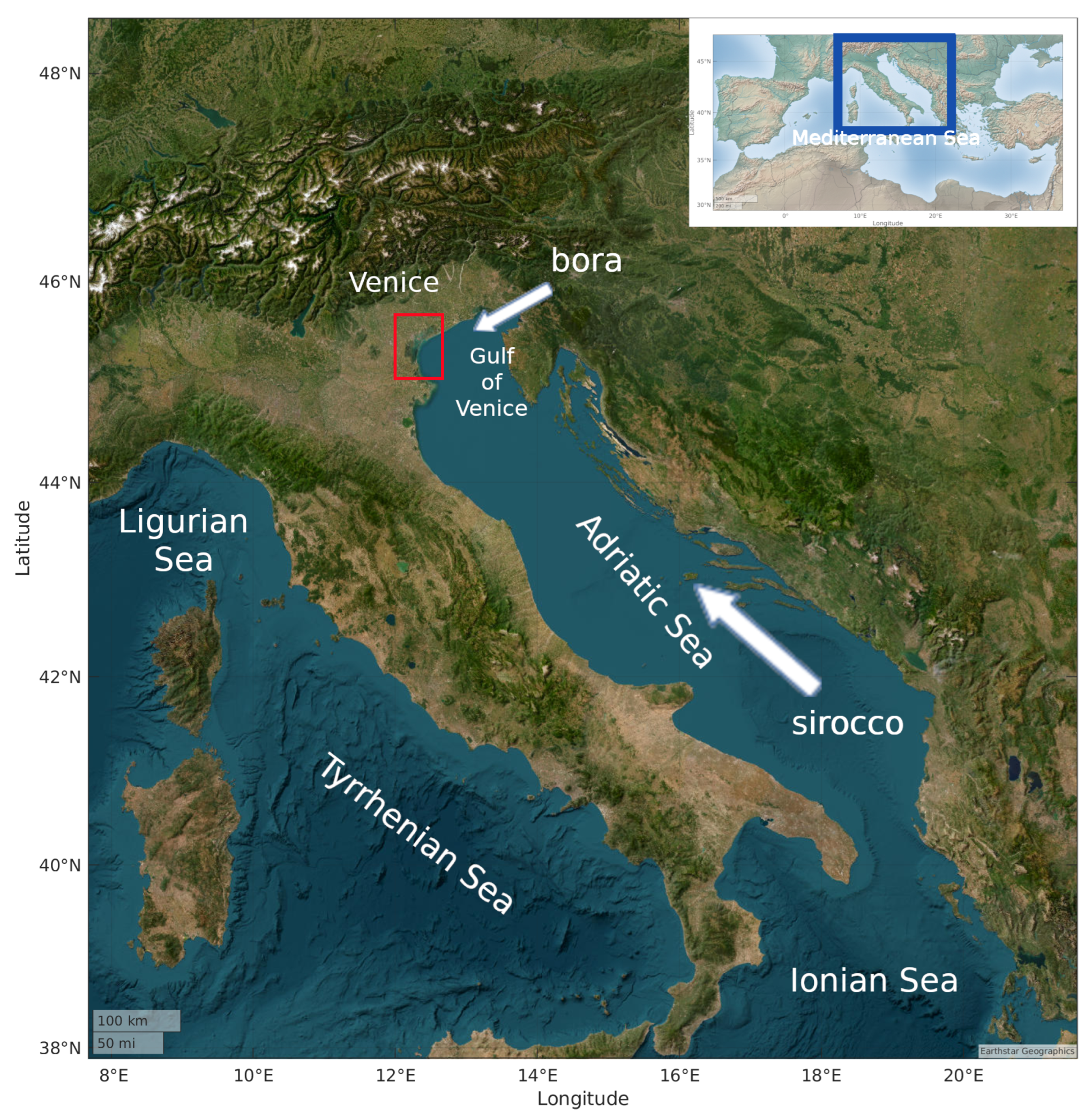
Figure 1. The Adriatic Sea bathymetry and its geographical orientation. Sirocco blows from the southeast, and bora from the northeast. In the northern part of the Adriatic Sea, the Gulf of Venice gathers the water pushed by storms from the southeast and northeast, triggering the high water at the coast and inside the Venice Lagoon. The red box marks the position of Venice and its lagoon. The inset map in the upper right corner shows the position of the Adriatic Sea inside the Mediterranean area, delimited by the blue box. Images by MathWorks MATLAB© software.
Jmse 11 00544 g001
Figure 2. The mean sea level and the annual number of high tides ≥ 110 cm registered in Venice in the period 1872–2021. Note: the MO.SE. system has been operational since December 2020 (Courtesy of Centro Previsioni e Segnalazioni Maree, Comune di Venezia).
Jmse 11 00544 g002
Figure 3. Scatterometer-ECMWF wind speed relative bias for the period January 2008 to November 2009. Scatterometer observations are from QuikSCAT and MetOP-A missions. Adapted from Figure 8 of [7].
Jmse 11 00544 g003
Figure 4. Distributions of the wind speed of scatterometer, standard forecast and the eight mitigated model forecasts for the SEVs of dataset D4. Black solid line: distribution of all the scatterometer winds falling into the D4 dataset. Black dash-dotted line: distribution of the standard forecast wind speeds. Other colors: winds related to the eight formulations of the MF, as per the legend.
Jmse 11 00544 g004
Figure 5. Mitigation factor ( 1 + Δ w N ) for the forecast of dataset D3. Ordinates in log scale. (a) MFs plot of the LLSR, RLSR, LLSR E and RLSR E mitigation approaches. (b) MFs plot of the other approaches.
Jmse 11 00544 g005
Figure 6. Taylor’s diagram showing the statistical indicators (cRMSD, linear correlation, standard deviation and bias) for the D3 dataset. Statistical indicators are calculated by considering all the pairs of observation-model as independent.
Jmse 11 00544 g006
Figure 7. Absolute error of the mitigated forecast and the scatterometer winds (SEV average) for dataset D3. The mitigated forecasts are drawn in orange and ordered by increasing absolute error of the standard forecast and the scatterometer winds (SEV average, in blue).
Jmse 11 00544 g007
Table 1. Summary of the statistical characteristics of the MF probability distributions. From left to right: model name, mean value, standard deviation, median value, skewness and kurtosis.
ModelMeanStd. Dev.MedianSkewnessKurtosis
L L S R 1.150.251.113.1736.79
R L S R 1.120.251.092.7131.28
L L S R E 1.120.231.093.0134.97
R L S R E 1.080.221.062.7532.90
O F 1.130.181.13−0.013.71
A F 1 1.411.061.2261.879531.17
A F 2 1.190.271.142.6126.16
A S 1.210.311.153.0532.90
Table 2. Bias of the wind speed of scatterometer and original forecast, and of the scatterometer and the eight different formulations of the mitigated forecasts (in ms 1 ). ( * ) SF stands for Standard Forecast.
Dataset#SF * LLSRRLSROFAF1AF2ASLLSR E RLSR E
D1290.950.110.210.04−0.21−0.01−0.030.240.38
D2480.970.160.300.10−0.150.060.030.270.45
D33640.840.240.340.19−0.020.160.130.330.46
D470.84−0.22−0.08−0.28−0.50−0.32−0.35−0.080.12
Table 3. RMSD of the mean wind speed of the scatterometer and original forecast, and of the scatterometer and the eight different formulations of the mitigated forecasts, grouped in SEVs (in ms 1 ).
Dataset#SFLLSRRLSROFAF1AF2ASLLSR E RLSR E
D1291.000.600.630.600.670.610.610.610.68
D2480.910.540.590.560.610.570.570.530.59
D33640.820.560.590.560.540.550.550.580.63
D470.780.390.370.430.510.430.430.380.37
Table 4. Success rate (%) of the eight formulations of the mitigation factor (in the columns) for each individual dataset (in the rows).
Dataset#LLSRRLSROFAF1AF2ASLLSR E RLSR E
D1297972727676767976
D2487973737175758175
D33647171737173737370
D4786718657868610086
Table 5. Bias and FR averaged over datasets and weighted by the number of cases in each dataset. Best performing cases are marked bold.
LLSRRLSROFAF1AF2ASLLSR E RLSR E
BIAS0.220.320.16−0.050.130.100.310.45
SR72.6171.2873.1471.1073.6173.6174.6771.17
Table 6. Bias and SR averaged over datasets D1, D2 and D4 and weighted by the number of cases in each dataset. Best performing cases are marked bold.
LLSRRLSROFAF1AF2ASLLSR E RLSR E
BIAS0.110.240.05−0.200.00−0.020.230.40
SR79.5872.4973.7471.5676.2676.2681.8976.26
Disclaimer/Publisher’s Note: The statements, opinions and data contained in all publications are solely those of the individual author(s) and contributor(s) and not of MDPI and/or the editor(s). MDPI and/or the editor(s) disclaim responsibility for any injury to people or property resulting from any ideas, methods, instructions or products referred to in the content.