Cause of Double-Peak Spectrum in Hyuga-Nada by the HF Radar

Abstract

High-frequency (HF) radar is a land-based instrument that can observe the radial distribution of oceanographic information, such as surface currents, wave heights, and wind directions. The first-order echo peak of the Doppler spectrum is often splits in this observation, and the levels of the split peaks are of approximately the same magnitude. We call this the double-peak spectrum. Because such a spectral shape may affect the derivation of oceanographic information, we examined the factors that cause double-peak spectra. The Kuroshio Current flows near the observation area of this study’s radar, which may have caused the double-peak spectrum. By mapping the spatial distribution of the double-peak spectra, we found areas in which the double-peak spectra occur relatively often at each radar station. The area of high vorticity ahead of the northeastward Kuroshio Current coincided with the area in which the double-peak spectra occurred, indicating the complexity of the currents occurring there; furthermore, more than two current velocity patterns can be mapped. These results show that the distance and directional continuity of the double-peak spectra can be used to calculate the flow-changing region with better spatial resolution.

1. Introduction

HF radar emits radio waves from antennas installed on land, ships, or other ocean platforms and receives the reflected signals. By analyzing the received reflected signals, it can observe surface currents, wave heights, wind directions, etc. with high spatiotemporal resolution.

Crombie [1] first observed a large, narrow peak within $\pm$1 Hz of the transmitted frequency in the spectrum of the reflected waves received from the ocean surface of HF-band radio waves. He concluded that this was a result of backscattering from ocean-surface waves traveling radially from the antenna with a half-wavelength relative to the wavelength of the transmitted radio wave, with the Doppler frequency corresponding to the phase velocity of the ocean surface waves.

Subsequently, the theoretical basis for backscattering at the ocean surface was established by Barrick [2,3], Hasselmann [4], and others. Stewart and Joy [5] used multiple frequencies and observed that the difference between the phase speed of backscattered radio waves and that of ocean waves over still water varied with the frequency. They showed good agreement between the observed current velocities and measured velocities of the drogue placed at that depth. These early studies established principles for measuring surface current velocities with HF radar and developed a system for mapping surface currents (e.g., Barrick et al. [6], Lipa and Barrick [7], Gurgel et al. [8]).

The Doppler spectrum of the backscattered signal obtained by the HF radar has two sharp peaks, called first-order echoes, around the Doppler frequency $\pm F_b$ corresponding to the phase velocity of ocean waves that satisfy the Bragg scattering resonance condition. These two first-order echoes were caused by waves propagating toward and away from the radar site. The Doppler frequency of the first-order echo corresponds to the speed of ocean wave movement; therefore, the difference between $\pm F_b$ values can be used to determine the surface current velocity in the radial direction of an observation cell.

The size of the HF radar observation cell can be determined by the distance and angular resolution. If a vortex or strong velocity shear is present in the observation cell, the first-order echo, which is usually a sharp peak, may broaden and split [9,10]. Double-peak spectra are often observed with this HF radar, where the first-order echo peak splits, and the levels of the split peaks are of approximately the same magnitude. A similar double-peak spectrum was also observed by Oshiro et al. [11] on an HF radar with a center frequency of 24.5 MHz, which was also located in Miyazaki.

Second-order harmonic peaks (SHPs) are a type of peak with high scattering intensities. Ivonin and Shrira [12] showed that SHPs are mainly caused by water waves that have the same wavelength as the transmitted radio waves and propagate parallel to the radar beam. The SHP appears at approximately $\sqrt{2}$ times the Doppler frequency from the first-order echo peak, and its power is approximately 20 dB lower than that of the first-order echo peak [13,14]. However, the observed double-peak spectrum is different from that of SHP because it is a strong power within approximately 10 dB of the first-order echo peak and does not necessarily appear at the $\sqrt{2}$-fold position.

When operating HF radar from a ship or other ocean platform, additional peaks appear in the Doppler spectrum that rival the first-order peaks, due to the motion of that platform [15,16]. However, that is not the cause of the double-peak spectrum because the HF radar used in this study is land-based.

One reason for the broadening of the first-order echo is the spatial variation in radial current velocity [17]. One possibility is that the antenna beam pattern may have caused broadening or splitting of first-order echoes. However, in the radar used in this study, the side lobes were more than 15 dB lower than the main lobes at all angles. Therefore, it is unlikely that the Doppler spectrum owing to the flow in the direction of the side lobes would appear as the second peak. The other is the spatial variation in the current velocity in the observation cell. The Kuroshio Current, a western boundary current of the North Pacific Ocean, flows near the observation area. Complex currents such as vortices and countercurrents can occur at the Kuroshio Current front. Double-peak spectra were observed when these events occurred in the observation area.

The purpose of this study is to examine the factors that cause the double-peak spectra observed by the 13.5 MHz radar from January 2019 to August 2021 and to show the possibility of mapping higher-resolution current velocities. First, we classified the double-peak spectra from the observed data to determine the incidence of occurrence. Next, we compared the monthly occurrence incidence of double-peak spectra with the positional relationship to the Kuroshio Current axis, which is a possible cause of the double-peak spectra. The spatial distribution of the double-peak spectrum was then calculated and compared with vorticity. Finally, we discuss the impact of the surface current measurements by mapping the surface current, assuming that each of the splitting peaks is a first-order echo.

2. Site and Dataset

2.1. Radar Specifications

The HF radar used in this study was installed in 2018 in Miyazaki Prefecture in Kyushu, Japan, and observed the Hyuga-Nada in the offshore area of eastern Kyushu Island. The radar system specifications of the two stations are listed in

Table 1. Specifications of two HF radar stations installed in Miyazaki Prefecture.

Center Frequency	13.5 MHz
Frequency sweep interval	0.5 s
Modulation method	Frequency Modulated Interrupted Continuous Wave
Sweep bandwidth	50 kHz
Beam-forming method	Multi-beam DBF in broadside array
Bearing resolution	±60° in step of 7.5°
Range resolution	3.0 km
Velocity resolution	4.34 cm/s
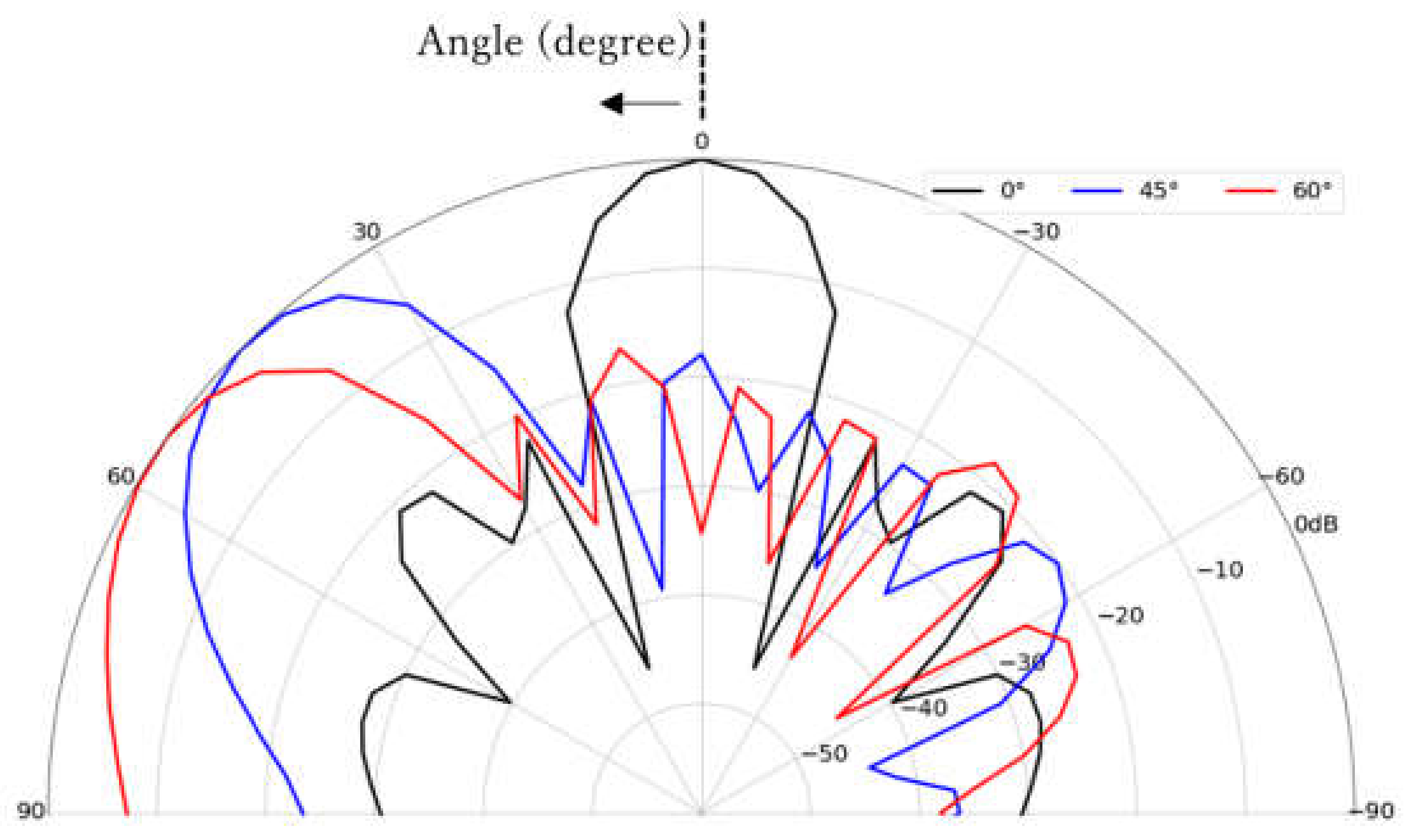
Antenna type	1 transmission of a 3-element Yagi and 8 receiving antennas of 2-element Yagis

. Each radar station consisted of one transmitting antenna and eight receiving antennas. The modulation method was a frequency-modulated interrupted continuous wave type, with a center frequency of 13.5 MHz and a sweep bandwidth of 50 kHz. Therefore, it had a range resolution of 3 km. The radar uses digital beamforming to observe an area of ±60° with $7.5°$ bearing resolution. The receive array antenna beam pattern is shown in Figure 1. It shows the antenna pattern when directivity is given to a boresight direction of 0 degrees (black line), 45 degrees (blue line), and 60 degrees (red line). At all angles, the side lobes are more than 15 dB lower than the main lobe.

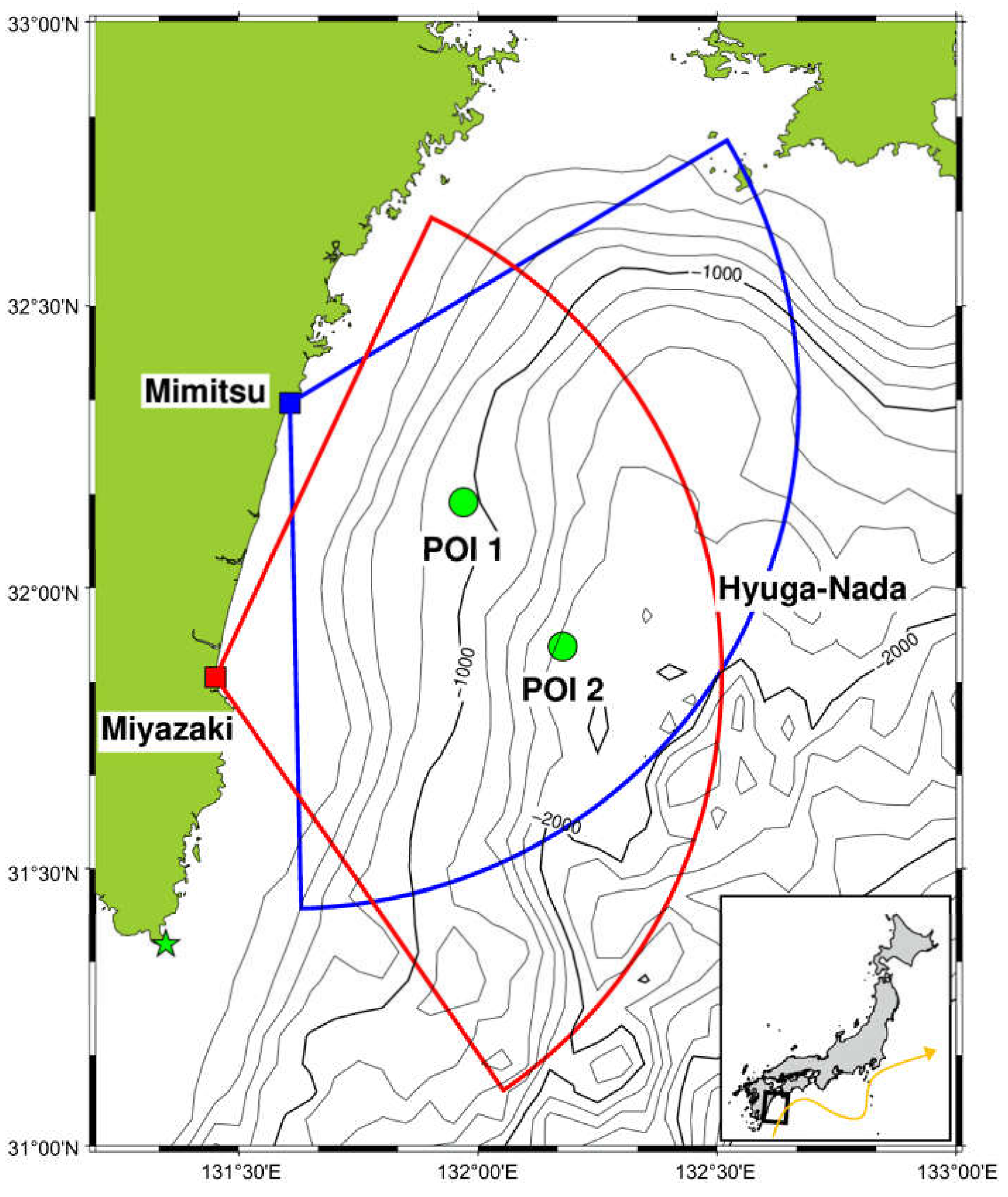
The locations and observation areas of the two radar stations are shown in Figure 2. The two radar stations are referred to as the Miyazaki and Mimitsu stations. The location of Miyazaki Station is indicated by a red square and that of Mimitsu Station is indicated by a blue square; the observation areas in all 17 azimuths are indicated by a fan shape. Each radar conducts observations hourly and maps surface currents and wave heights. Here, we report an analysis of the dataset obtained by these two radar stations from January 2019 to August 2021.

2.2. Example of the Double-Peak Spectrum

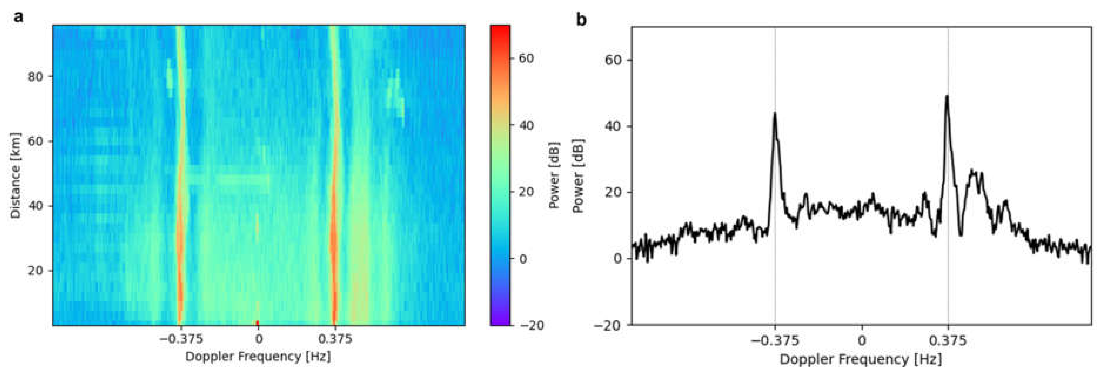
Figure 3 shows a typical Doppler spectrum. Figure 3a shows the Doppler spectrum from 3 to 96 km (range-Doppler spectrum) of beam 8 at 08:00 (JST) on 2 November 2020 at Miyazaki Station. The horizontal axis represents the Doppler frequency [Hz], the vertical axis represents the distance from the radar [km], and the color bar represents the signal power [dB]. The beam number was set to 0 for the direction of the most southerly radio-wave radiation and 16 for the most northerly. In Figure 3a, first-order peaks appear in the positive and negative frequency regions at each distance. Figure 3b shows the Doppler spectrum of Figure 3a at 51 km. The horizontal axis represents the Doppler frequency [Hz], and the vertical axis represents the signal power [dB]. A sharp peak caused by Bragg scattering resonance is observed around ±${\mathit{F}}_{\mathit{b}}$, which is calculated from the phase velocity of the ocean waves satisfying the Bragg resonance condition, as in the following equation:

$${\mathit{F}}_{\mathit{b}}=\frac{\mathbf{2}\mathit{f}}{\mathit{c}}\times \sqrt{\frac{\mathit{g}\mathit{\lambda }}{\mathbf{4}\mathit{\pi }}}=\frac{\mathbf{2}\times \mathbf{13.5}\times {\mathbf{10}}^{\mathbf{6}}}{\mathbf{3}\times {\mathbf{10}}^{\mathbf{8}}}\times \sqrt{\frac{\mathbf{9.8}\times \mathbf{22.2}}{\mathbf{4}\times \mathit{\pi }}}\cong \mathbf{0.375},$$

(1)

where $\mathit{f}$ is the center frequency of the transmitted radio wave, $\mathit{c}$ is the radio wave velocity, $\mathit{g}$ is the acceleration due to gravity, and $\mathit{\lambda }$ is the wavelength of the transmitted radio wave.

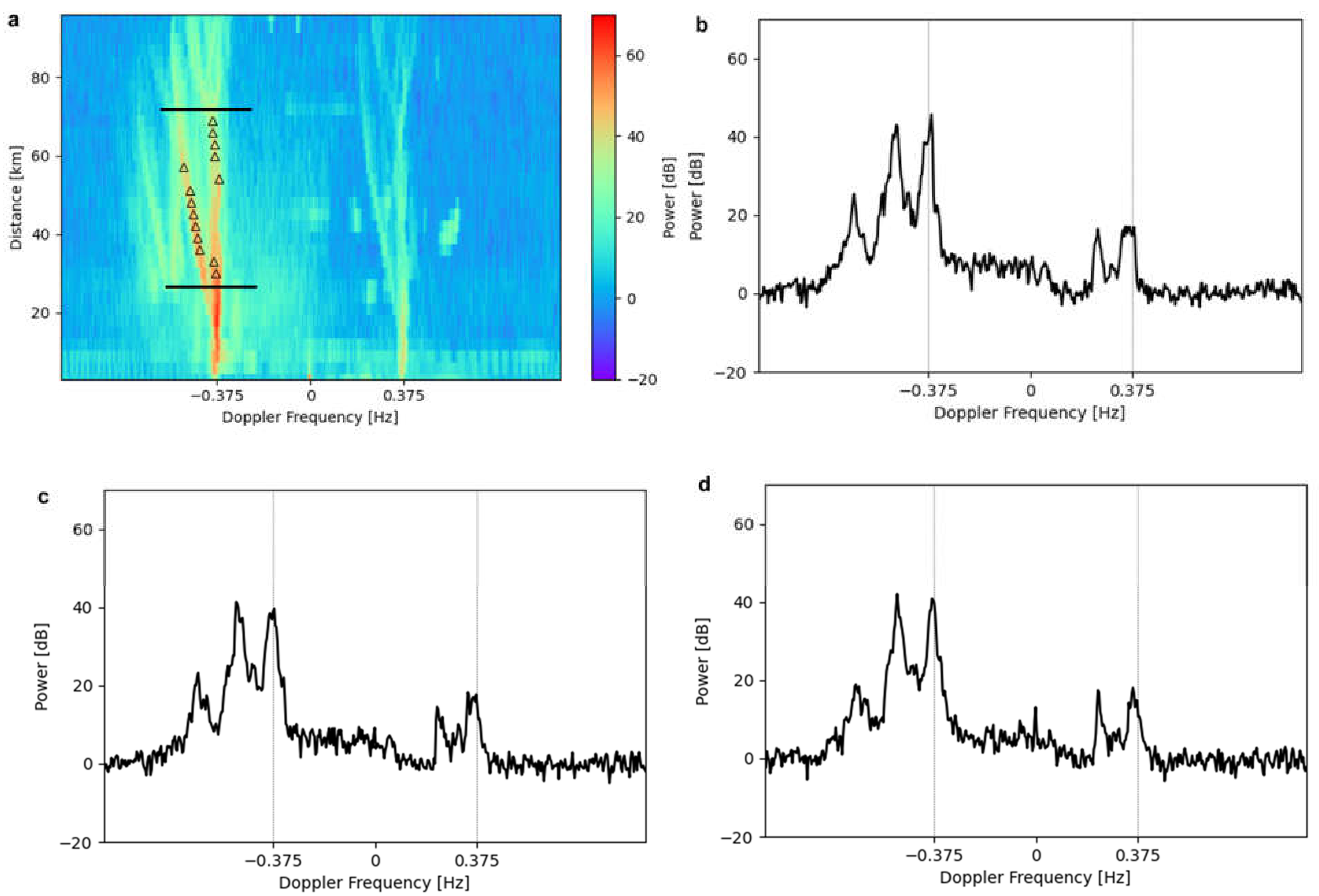
Figure 4 shows an example of the observed double-peak spectrum. Figure 4a shows the range-Doppler spectrum of beam 12 at 14:00 (JST) on 19 January 2019 at the Miyazaki Station. In Figure 4a, the peak splits from approximately 30 km, and another peak with almost the same power as the first-order peak can be observed until approximately 70 km. Figure 4b–d show the Doppler spectra of the 54, 57, and 60 km points in Figure 4a, where a peak near $\pm {\mathit{F}}_b$ and another peak away from it can be seen. The split peaks changed with each distance. Therefore, when deriving oceanographic information such as the current velocity, the calculation results will change with distance. For example, if the radial velocity $\mathit{V}$ is obtained from the first-order peak at each distance using the following equation, Figure 4b is 8.67 cm/s, Figure 4c is −147.42 cm/s, and Figure 4d is −8.67 cm/s. As such, there was a large difference in the flow velocity at successive distances. Equation (2) demonstrates this as follows:

$$\mathit{V}=\frac{\mathit{c}}{\mathbf{2}\mathit{f}}\left({\mathit{f}}_{\mathbf{1}}\mathit{\pm }{\mathit{F}}_{\mathit{b}}\right)=\frac{\mathbf{3}\mathit{\times }{\mathbf{10}}^{\mathbf{8}}}{\mathbf{2}\times \mathbf{13.5}\times {\mathbf{10}}^{\mathbf{6}}}\times \left({\mathit{f}}_{\mathit{1}}\pm \mathbf{0.375}\right),$$

(2)

where ${\mathit{f}}_{\mathbf{1}}$ denotes the Doppler frequency of the first peak at each distance. The $\pm$ sign in Equation (2) is positive when ${\mathit{f}}_{\mathbf{1}}<\mathbf{0}$ and negative when ${\mathit{f}}_{\mathbf{1}}>\mathbf{0}$.

3. Analysis of Double-Peak Spectrum

3.1. Classifying Double-Peak Spectra

To calculate the incidence and spatial distribution of the double-peak spectra, it is necessary to classify them within the dataset. However, the observed data were generated for 17 azimuths per hour; that is 400,000 per station from January 2019 to August 2021, which is enormous. Therefore, the following algorithm was used to classify the double-peak spectra, where $\mathit{i}$ is the cell number in the distance and $\mathit{j}$ is the number of points in the Doppler frequency (1–512 points). The power of the first-order peak is ${\mathit{P}}_{\mathbf{1}}\left(\mathit{i}\right)$, that of the second-order peak is ${\mathit{P}}_{\mathbf{2}}\left(\mathit{i}\right)$ at each distance, and that at each point in the Doppler frequency is $\mathit{P}\left(\mathit{i},\mathit{j}\right)$. The algorithm is:

i.

Smoothing of the Doppler frequency to remove small noise disturbances. In this study, the number of moving averages in smoothing was five;

ii.

Detecting ${\mathit{P}}_{\mathbf{1}}\left(\mathit{i}\right)$ and ${\mathit{P}}_{\mathbf{2}}\left(\mathit{i}\right)$ within the ±2 m/s range in radial velocity;

iii.

The observed data showed a sharp first peak in most cases, at least up to 60 km. We recorded the difference between ${\mathit{P}}_{\mathbf{1}}\left(\mathit{i}\right)$ and the mean value of power outside the ±2 m/s range in the radial velocity for one year and calculated its mean ${\mathit{\mu }}_{\mathbf{60}}$ and standard deviation ${\mathit{\sigma }}_{\mathbf{60}}$ at 60 km. Comparing the ${\mathit{P}}_{\mathbf{1}}\left(\mathit{i}\right)$ with the average value of power outside the ±2 m/s range in the radial velocity to determine whether the following conditions are met:

$${\mathit{P}}_{\mathbf{1}}\left(\mathit{i}\right)>\frac{{{\displaystyle \sum }}_{\mathit{j}=\mathbf{1}}^{\mathit{j}=\mathbf{114}}\mathit{P}\left(\mathit{i},\mathit{j}\right)+{{\displaystyle \sum }}_{\mathit{j}=\mathbf{208}}^{\mathit{j}=\mathbf{306}}\mathit{P}\left(\mathit{i},\mathit{j}\right)+{{\displaystyle \sum }}_{\mathit{j}=\mathbf{400}}^{\mathit{j}=\mathbf{512}}\mathit{P}\left(\mathit{i},\mathit{j}\right)}{\mathbf{417}}+\left({\mathit{\mu }}_{\mathbf{60}}-\mathbf{2}{\mathit{\sigma }}_{\mathbf{60}}\right);$$

In this study, ${\mathit{\mu }}_{\mathbf{60}}-\mathbf{2}{\mathit{\sigma }}_{\mathbf{60}}$ was set at 25dB.

iv.

Comparing the ${\mathit{P}}_{\mathbf{1}}\left(\mathbf{i}\right)$ with the average value of power within the ±2 m/s range in the radial velocity to determine whether the following conditions are met:

$$\begin{gathered} \mathrm{if} {\mathit{f}}_{\mathbf{1}}<\mathbf{0} {\mathit{P}}_{\mathbf{1}}\left(\mathit{i}\right)>\frac{{{\displaystyle \sum }}_{\mathit{j}=\mathbf{115}}^{\mathit{J}=\mathbf{207}}\mathit{P}\left(\mathit{i},\mathit{j}\right)}{\mathbf{47}}+\mathbf{10} dB, \\ \mathrm{if} {\mathit{f}}_{\mathbf{1}}>\mathbf{0} {\mathit{P}}_{\mathbf{1}}\left(\mathit{i}\right)>\frac{{{\displaystyle \sum }}_{\mathit{j}=\mathbf{307}}^{\mathit{J}=\mathbf{399}}\mathit{P}\left(\mathit{i},\mathit{j}\right)}{\mathbf{47}}+\mathbf{10} dB; \end{gathered}$$

v.

Comparing the ${\mathit{P}}_{\mathbf{1}}\left(\mathbf{i}\right)$ with the power outside the ±2 m/s range in radial velocity to determine whether the following conditions are met:

$${\mathit{P}}_{\mathbf{1}}\left(\mathit{i}\right)>\mathit{P}\left(\mathit{i},\mathit{j}\right)+\mathbf{10} dB \left(\mathbf{1}\le \mathit{j}\le \mathbf{114} and \mathbf{208}\le \mathit{j}\le \mathbf{306} and \mathbf{400}\le \mathit{j}\le \mathbf{512}\right),$$

Use these iii, iv, and v conditions to remove cases where not enough peaks appear or where there is too much noise;

vi.

Because the split peaks in the double-peak spectrum have nearly the same power, determine whether the following conditions are met:

$${\mathit{P}}_{\mathbf{2}}\left(\mathit{i}\right)>{\mathit{P}}_{\mathbf{1}}\left(\mathit{i}\right)-\mathbf{10}dB;$$

vii.

Assuming that the double-peak spectrum is a spectrum in which the first-order echo peak splits into two, not noise that appears around the first-order echo peak. We think that the spectrum between the peaks is the shape of a valley and determine whether the power minimum ${\mathit{P}}_{\mathit{m}\mathit{i}\mathit{n}}$ between the first-order and second-order peaks in the frequency direction satisfies the following conditions:

$${\mathit{P}}_{\mathit{m}\mathit{i}\mathit{n}}\left(\mathit{i}\right)<{\mathit{P}}_{\mathbf{2}}\left(\mathit{i}\right)-\mathbf{5}dB;$$

viii.

Assuming that the double-peak spectrum is continuous in distance, determine whether the double-peak spectrum occurs continuously at a total of three points at that distance and at the front and rear distances.

Table 2. Classification results for double-peak spectra from January 2019 to August 2021.

Year	Mimitsu Station		Miyazaki Station
	Number	Rate [%]	Number	Rate [%]
Jan.–Dec. 2019	20,843	14.02	26,934	18.42
Jan.–Dec. 2020	16,138	10.82	17,288	11.72
Jan.–Aug. 2021	11,784	11.89	12,686	12.86

shows the results of classifying the double-peak spectra using the data observed at the two stations from January 2019 to August 2021. The number of double-peak spectra for both stations was less than 20% in all years, with Miyazaki Station observing more instances than Mimitsu Station did.

3.2. Relationship to the Kuroshio Current Axis

We defined the incidence of double-peak spectra ${\mathit{D}}_{\mathit{a}}\left(\mathit{t}\right)$ at each radar station as the ratio of the number of occurrences to the number of observations during the selected period:

$${\mathit{D}}_{\mathit{a}}\left(\mathit{t}\right)=\frac{{{\displaystyle \sum }}_{\mathit{t}}{{\displaystyle \sum }}_{\mathit{\theta }}\mathit{N}\left(\mathit{\theta },\mathit{t}\right)}{{\mathit{N}}_{\mathit{a}\mathit{l}\mathit{l}}},$$

(3)

where ${\displaystyle \sum }_{\mathit{t}}{\displaystyle \sum }_{\mathit{\theta }}\mathit{N}\left(\mathit{\theta },\mathit{t}\right)$ is the number of double-peak spectrum occurrences during the selected period for each radar station. $\mathit{\theta }$ is the azimuth angle, and $\mathit{t}$ is the period. ${\mathit{N}}_{\mathit{a}\mathit{l}\mathit{l}}$ denotes the maximum number of numerators. For example, ${\mathit{N}}_{\mathit{a}\mathit{l}\mathit{l}}$ when calculating ${\mathit{D}}_{\mathit{a}}\left(\mathit{t}\right)$ for January 2019 is 17 azimuths × 24 h × 31 days, which is 12,648.

Figure 5 shows ${\mathit{D}}_{\mathit{a}}\left(\mathit{t}\right)$ for each month. The vertical axis shows the occurrence incidence, the horizontal axis shows the monthly change, and the blue and red lines show the monthly incidences of Mimitsu Station and Miyazaki Station, respectively. The monthly incidence of double-peak spectra at both stations showed the same trend of change. The 2019 fluctuation trend was lowest in August and very high in January and December. In 2021, the incidence was high in January and February but was sharply lower in March.

The Kuroshio Current axis location was similar to the change in ${\mathit{D}}_{\mathit{a}}\left(\mathit{t}\right)$. Figure 6 shows the distance to the Kuroshio Current axis and the incidence of the double-peak spectra from January 2019 to August 2021. The green line shows the distance to the Kuroshio Current axis from Cape Toi by the Japan Coast Guard [18], and the red line shows the daily ${\mathit{D}}_{\mathit{a}}\left(\mathit{t}\right)$ at Miyazaki Station. The correlation coefficient was −0.4791, indicating a negative correlation. In January and December 2019, when many double-peak spectra occurred, the distance to the Kuroshio Current axis was close to the shore, whereas, in July and August 2019, when few double-peak spectra occurred, the Kuroshio Current axis was away from the shore. In 2021, the Kuroshio Current axis was close to the shore in January and February but moved away from the shore significantly in March, showing a large change in a short period of time, similar to the incidence of the double-peak spectrum. As shown above, the incidence of the double-peak spectra and the Kuroshio Current axis location are similar in their characteristic changes.

3.3. Spatial Distribution

We defined the incidence of double-peak spectra ${\mathit{D}}_{\mathit{c}}\left(\mathit{m}, \mathit{\theta }, \mathit{t}\right)$ in each observation cell (denoted by the distance $\mathit{m}$ from each radar station and azimuth angle $\mathit{\theta }$) as the ratio of the number of occurrences to the number of observed data points during the selected period $\mathit{t}$ in each observation cell:

$${\mathit{D}}_{\mathit{c}}\left(\mathit{m},\mathit{\theta },\mathit{t}\right)=\frac{{{\displaystyle \sum }}_{\mathit{t}}\mathit{N}\left(\mathit{m},\mathit{\theta },\mathit{t}\right)}{{\mathit{N}}_{\mathit{a}\mathit{l}\mathit{l}}},$$

(4)

where ${\displaystyle \sum }_{\mathit{t}}\mathit{N}\left(\mathit{m},\mathit{\theta },\mathit{t}\right)$ is the number of occurrences of the double-peak spectra in the selected period for each observation cell. 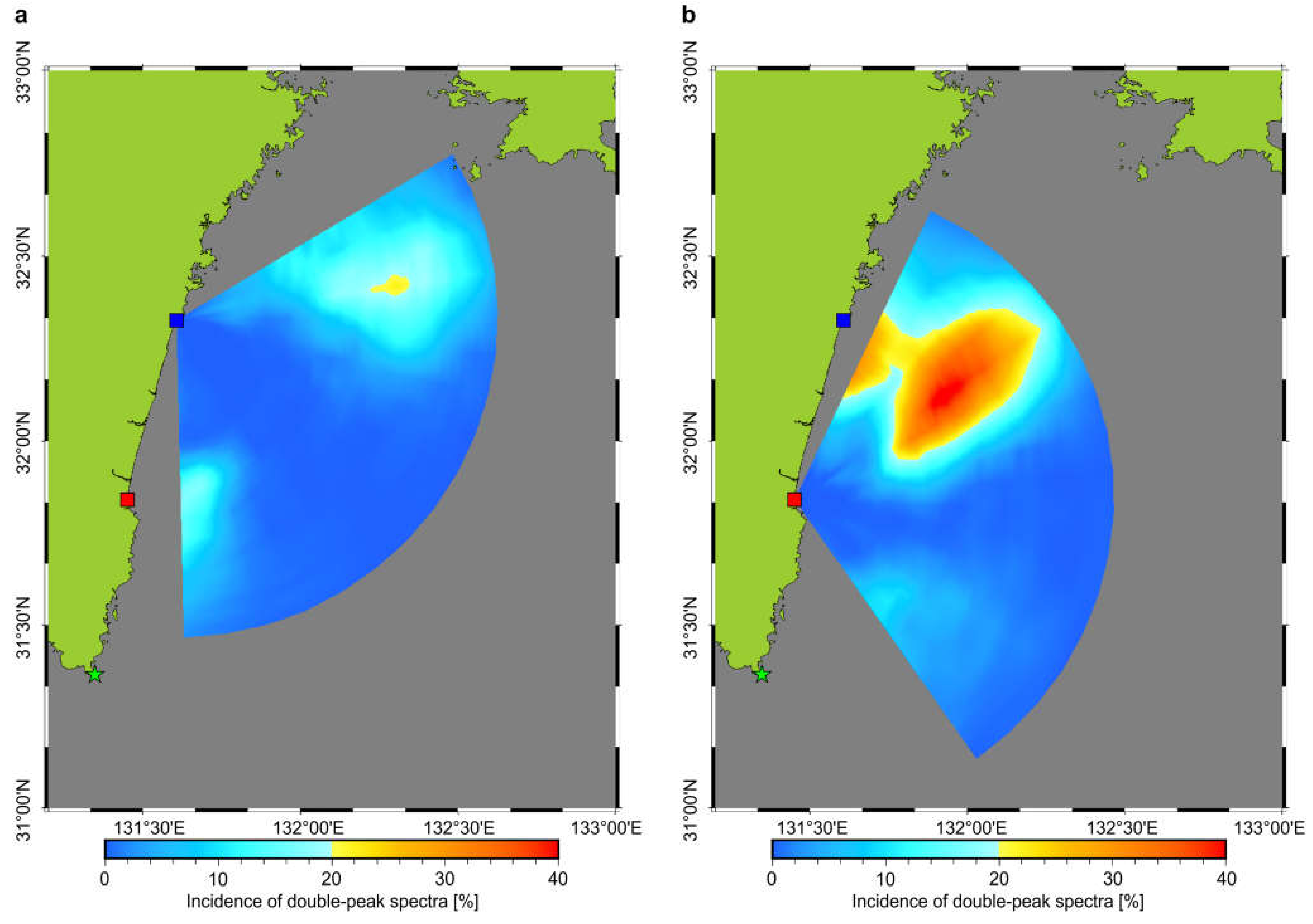The spatial distribution plot of the double-peak spectrum for January 2019 created by ${\mathit{D}}_{\mathit{c}}\left(\mathit{m}, \mathit{\theta }, \mathit{t}\right)$ calculated for each observation cell is shown in Figure 7. Figure 7a,b show the results for Mimitsu and Miyazaki Stations, in which the incidence is higher on the north side for both cases. An area with a high incidence of double-peak spectra in Figure 7b existed in the direction of the bore site in Figure 7a, but almost no double-peak spectra were generated. However, the distant area in the direction of its high incidence in Figure 7b also had high incidence in Figure 7a.

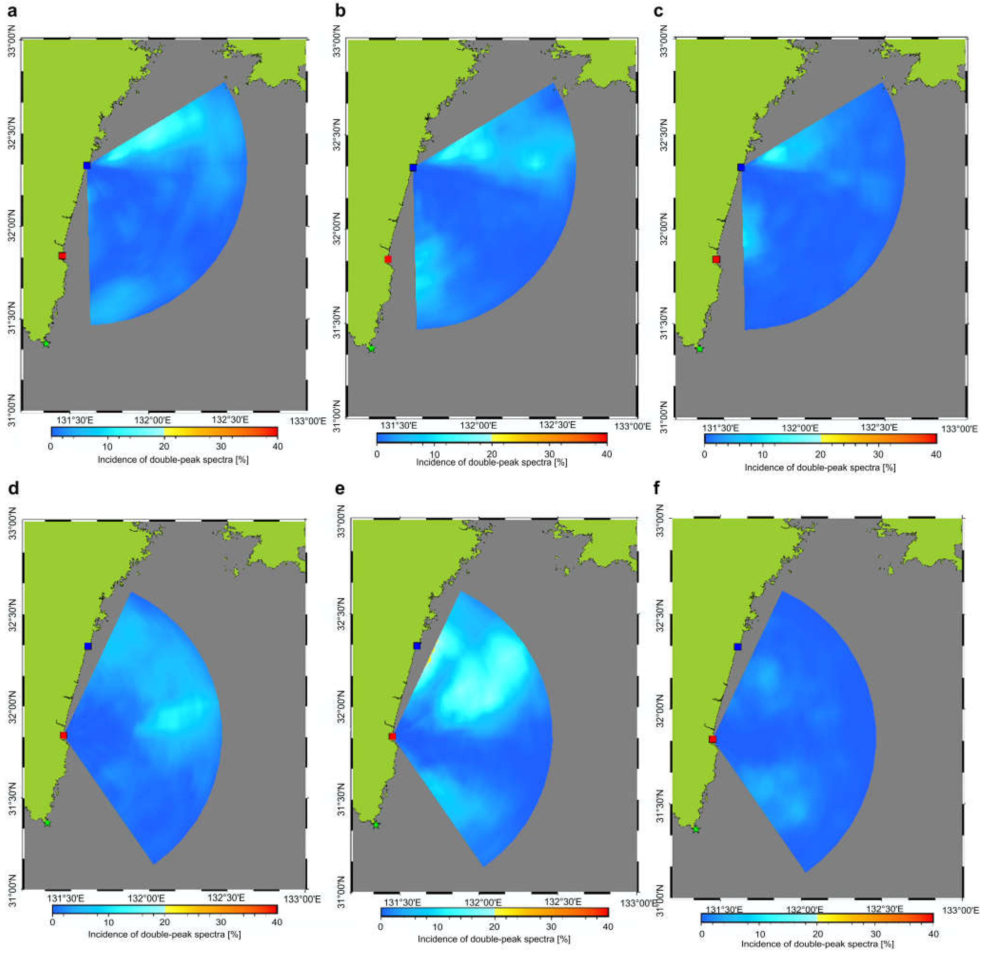
Figure 8 shows the change in the spatial distribution of the double-peak spectrum every two months for period ① shown in Figure 6. In period ① of Figure 6, the Kuroshio Current axis moves away from the shore as a change from March to July 2019. In Figure 8, the area with a high incidence of double-peak spectra disappears, and the number of occurrences decreases. Figure 9 shows the change in the spatial distribution of the double-peak spectrum for period ② shown in Figure 6. In period ② of Figure 6, the Kuroshio Current axis moves close to the shore as a change from January to February 2021, and then it moves away from the shore significantly in March 2021. Figure 9 shows that the area with a high incidence of double-peak spectra moved close to the shore from January to February. However, in March 2021, an area with a high incidence of double-peak spectra was no longer observed in the study area. Thus, the double-peak spectrum does not occur in a specific area, and the area with a high incidence changes with the position of the Kuroshio Current axis.

There are two possible reasons for areas in which the incidence of double-peak spectra is high at Miyazaki Station but low at Mimitsu Station in Figure 7, Figure 8 and Figure 9. First, the current can be seen differently, depending on the radar location and azimuth angle. There are cases in which the currents can be perceived as two different currents, as shown in Figure 10a, and cases in which they can be perceived as almost the same current, as shown in Figure 10b. The second factor is related to the size of the HF radar observation cell. As shown in Figure 11, the observation cell is spread out, and two currents are observed at a far distance, but only one current may be observed in the near distance because the observation cell is narrower.

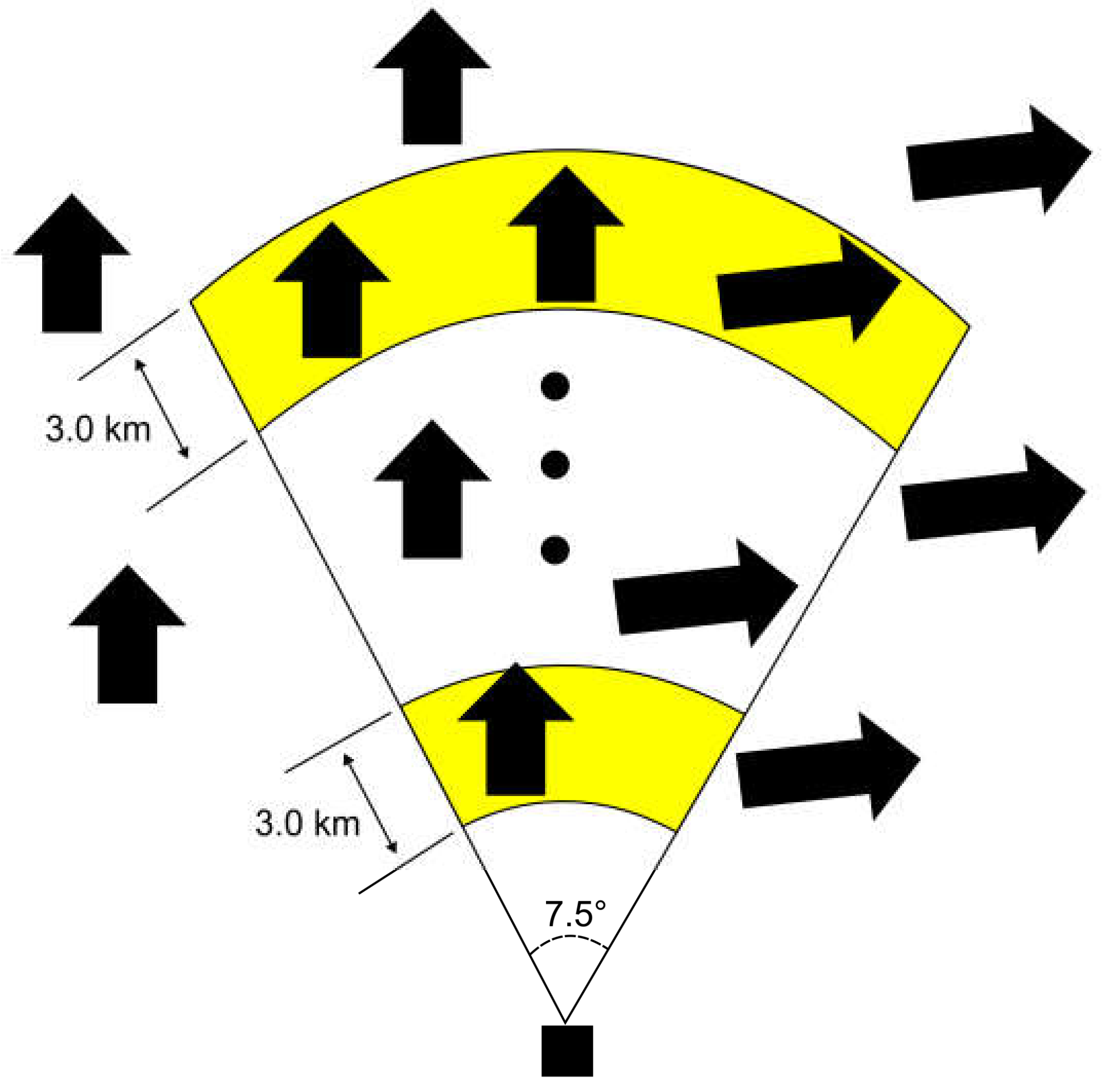
3.4. Vorticity and Incidence of Double-Peak Spectra

We discuss the relationship between the area in which the flow changes and the area in which the double-peak spectrum is generated in terms of vorticity because the double-peak spectrum is considered to observe vortex or velocity shear. The vorticity $\mathit{\zeta }\left[{\mathit{s}}^{-\mathbf{1}}\right]$ was calculated at each grid point for which the current was sought using the following equation:

$$\begin{array}{c}\hfill \Delta \mathit{V}={\mathit{V}}_{\mathit{east}}-{\mathit{V}}_{\mathit{west}}\\ \hfill \Delta \mathit{U}={\mathit{U}}_{\mathit{north}}-{\mathit{U}}_{\mathit{south}},\\ \hfill \mathit{\zeta }\left[{\mathit{s}}^{-\mathbf{1}}\right]=\frac{\Delta \mathit{V}}{\Delta \mathit{x}}-\frac{\Delta \mathit{U}}{\Delta \mathit{y}}\end{array}$$

(5)

where $\Delta \mathit{x}$ and $\Delta \mathit{y}$ are 6 km, and ${\mathit{V}}_{\mathit{e}\mathit{a}\mathit{s}\mathit{t}}$ and ${\mathit{V}}_{\mathit{w}\mathit{e}\mathit{s}\mathit{t}}$ are the V components of the current 3 km to the west and east from the point at which the vorticity is calculated. ${\mathit{U}}_{\mathit{s}\mathit{o}\mathit{u}\mathit{t}\mathit{h}}$ and ${\mathit{U}}_{\mathit{n}\mathit{o}\mathit{r}\mathit{t}\mathit{h}}$ are the U components of the current 3 km south and north, respectively, from the point at which the vorticity is calculated. 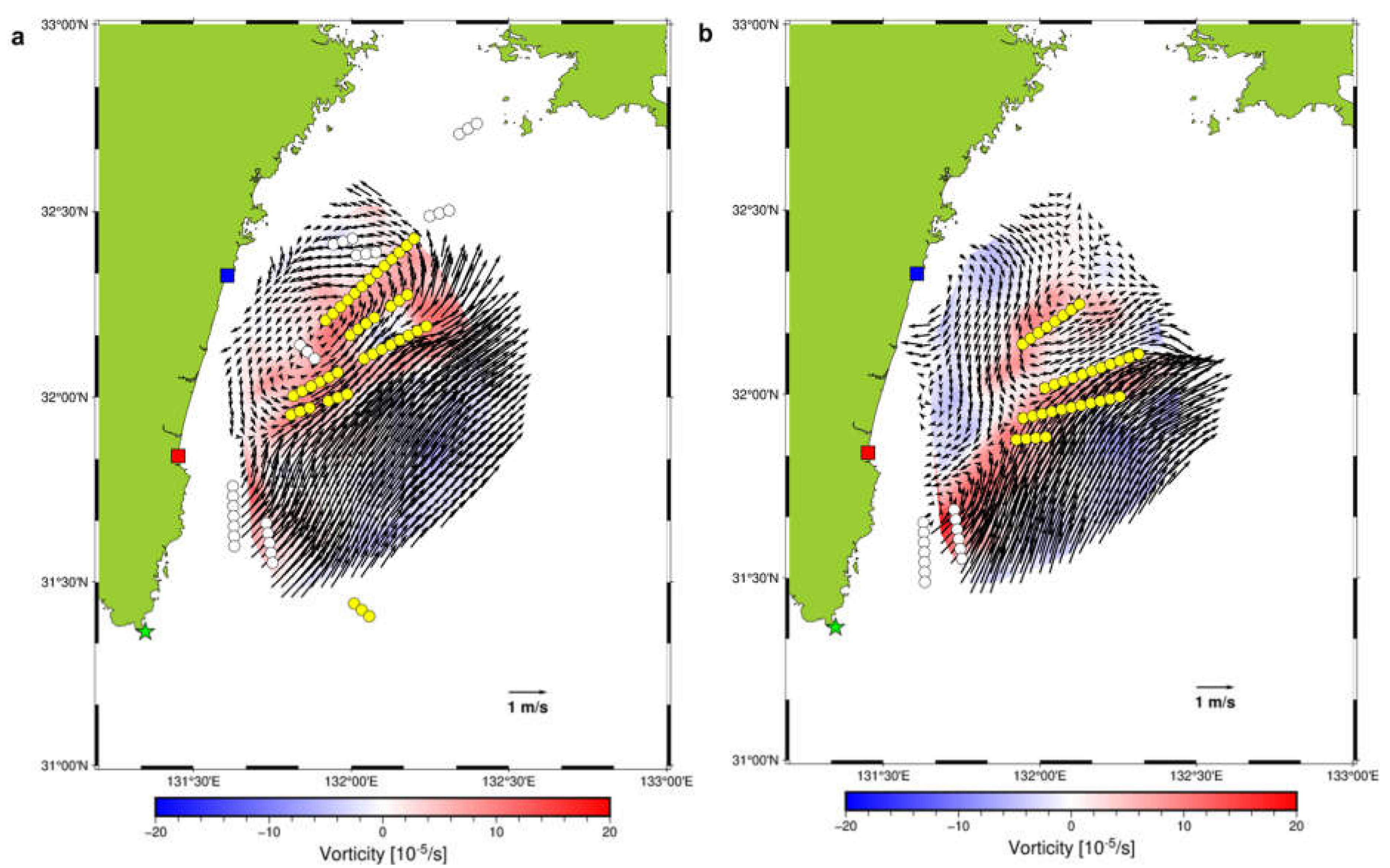Figure 12 shows an example of a vorticity map calculated at each grid point. The black arrows are the current velocities, the colored bars are the vorticity, and the yellow and white circles are the areas in which the double-peak spectra occurred at the Miyazaki and Mimitsu stations. In both Figure 12a,b, the vorticity was higher in areas at which the Kuroshio Current—flowing close to the shore—significantly changed the current. This area coincided with the area at which the double-peak spectra occurred. The areas in which double-peak spectra occurred at Miyazaki Station are in particularly good agreement with the areas of high vorticity. This is thought to be because the front area of the Kuroshio Current when close to the shore is parallel to the beam direction at Miyazaki Station, and there are many situations in which there are two currents in the observation cell at consecutive distances.

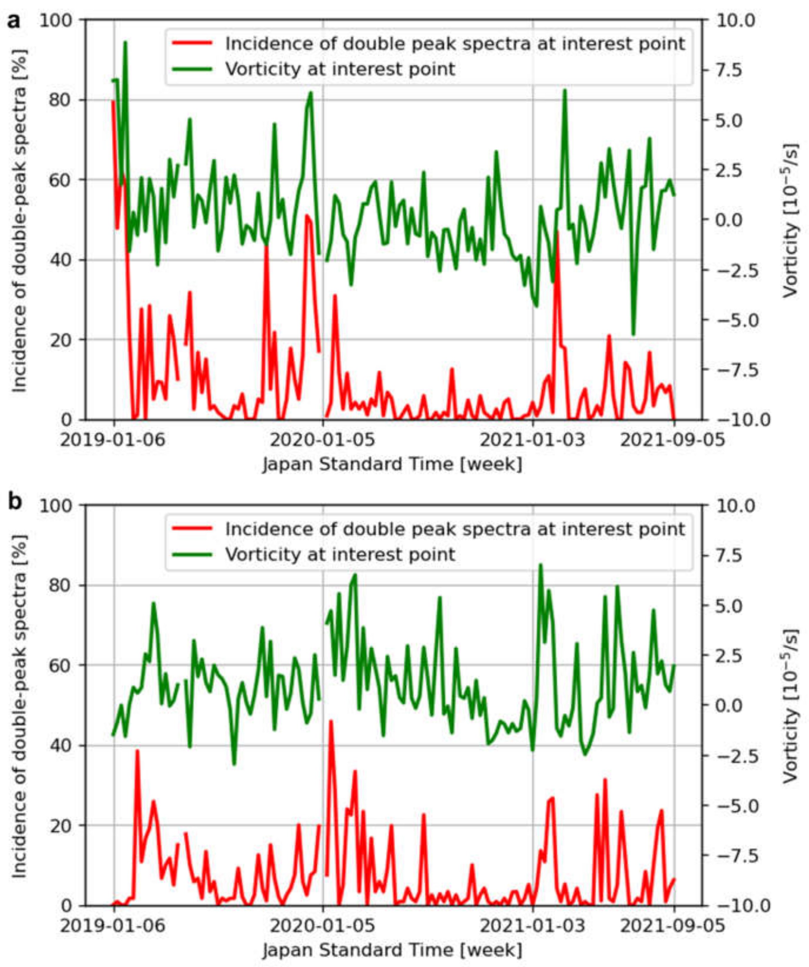
Figure 13 compares the vorticity and double-peak occurrence rate of Miyazaki Station on a weekly average basis, focusing on POI 1 and POI 2 in Figure 2. Figure 13a shows the results at POI 1 with a correlation coefficient of 0.5779. High vorticity periods, such as January and December 2019, coincide with periods when the Kuroshio Current flows close to the shore, and the incidence of double-peak spectra tends to be higher at those times. Figure 13b shows the results for POI 2, with a correlation coefficient of 0.5617. In Figure 13a, both the vorticity and double-peak spectra were higher in January 2019, whereas, in Figure 13b, both were lower in January 2019, and both were higher in March 2019. Similarly, for other periods, Figure 13b shows that the period when both vorticity and double-peak spectra incidence are high is approximately two months later than that in Figure 13a. This is thought to be because the incidence of double-peak spectra increases when the Kuroshio Current front area coincides with the area of interest.

Figure 14 shows the results of mapping the current velocity in the area where the double-peak spectrum occurred in Figure 13a using the first and second peaks. The areas in which the currents were different in Figure 14a,b, owing to the effect of the double-peak spectra, were divided into three areas. AREA1 and AREA2 are the composite results of the radial velocity obtained from the two peaks observed at Miyazaki Station and the first peak observed at Mimitsu Station. AREA3 is the result of compositing the radial velocity obtained from the first peak observed at Miyazaki Station and the two peaks observed at Mimitsu Station. In AREA1 and AREA3, Figure 14a shows the Kuroshio Current in a northeasterly direction, while Figure 14b shows the current in a southerly or southwesterly direction. In AREA 2, the same northeastward current is approximately 0.5 m/s in Figure 14a but more than 1 m/s in Figure 14b, showing a significant difference in current strength. These results indicate that more than one current was present in the area in which the double-peak spectra occurred.

4. Conclusions

We used data from 13.5 MHz radars observing the Hyuga-Nada Sea off the eastern coast of Kyushu, Japan. In general, the Doppler spectrum obtained from observations has a sharp peak called the first-order echo; however, in this observation area, the Doppler spectrum often splits this peak and has another peak with almost the same power as the first-order echo peak. We call this the double-peak spectrum. The reason for the broadening and splitting of the first-order echo spectrum is thought to be the presence of a vortex or velocity shear in the observation cell. In this study, we examined the factors that cause the observed double-peak spectra using its incidence rate, spatial distribution, and comparison with vorticity.

First, we defined the conditions for the double-peak spectra and classified them based on the observed data of two stations from January 2019 to August 2021. The classification results showed that the incidence of double-peak spectra was higher at Miyazaki Station than at Mimitsu Station for all years. The monthly variations in the incidence of the double-peak spectra at the two stations were the same. In 2019, the incidence of the double-peak spectrum was higher in January and December but lowest in August. In 2021, the incidence of the double-peak spectrum was high in January and February but decreased significantly in March. Resembling this fluctuation trend was the Kuroshio Current axis position. According to the Japan Coast Guard, the distance from Cape Toi to the Kuroshio Current axis was close to the shore in January and December 2019 and away from the shore in July and August. In January and February 2021, it was close to the shore, but significantly away from the shore in March. It was found that the double-peak spectrum is related to the distance of the Kuroshio Current from the shore because the characteristics of the change are consistent with each other.

By creating a monthly spatial distribution of the double-peak spectra, we found that there are areas in which double-peak spectra occur more often for each radar station and that these areas change from month to month. Both radar stations have many double-peak spectra in the northern part of the observation area. There were areas in which many double-peak spectra were observed at one radar station but almost no double-peak spectra were observed at the other radar station. This could be attributed to two reasons. One is the possibility that two currents in one observation cell may be perceived as almost the same current, depending on the location of the radar station and beam direction. Another possibility is that two currents are observed at far distances because the observation cell is spread out, but only one current is observed at close distances because the observation cell is narrower.

We verified that double-peak spectra were observed in areas of changing currents by comparing the areas in which double-peak spectra were observed with the vorticity distribution. In this area, the Kuroshio Current flows toward the northeast; therefore, the vorticity tends to be high in its front area. The areas in which double-peak spectra were observed coincided well with the areas of high vorticity. Comparing the incidence of double-peak spectra and vorticity from January 2019 to August 2021 at the points of interest, the periods when both were high coincided with each other. This suggests that the incidence of the double-peak spectra increases when the Kuroshio front area coincides with the area of interest.

We revealed the spatial distribution of the current velocity using each peak of the double-peak spectrum. As a result, there were areas where the northeastward Kuroshio Current and the southward current could be observed simultaneously, as well as areas where the direction of the current was the same but the speeds were very different. This indicates that the double-peak spectra observed by this radar mainly occurred when areas with large velocity differences at the front of the Kuroshio Current were present in the observation cell.

As further research, we would like to identify the area where the flow in the observation cell changes according to continuity of distance, direction, and time in the area where the double-peak spectrum is occurred. To identify this, we are also considering using high-resolution direction-finding methods such as MUSIC to investigate the azimuth angle of each peak in the double-peak spectrum. This would allow us to obtain higher spatial resolution by using both the first and second peaks of the double-peak spectrum to determine the current velocity.