


Normal Operating Performance Study of 15 MW Floating Wind Turbine System Using Semisubmersible Taida Floating Platform in Hsinchu Offshore Area


Abstract
1. Introduction
2. Wind Turbine System Design
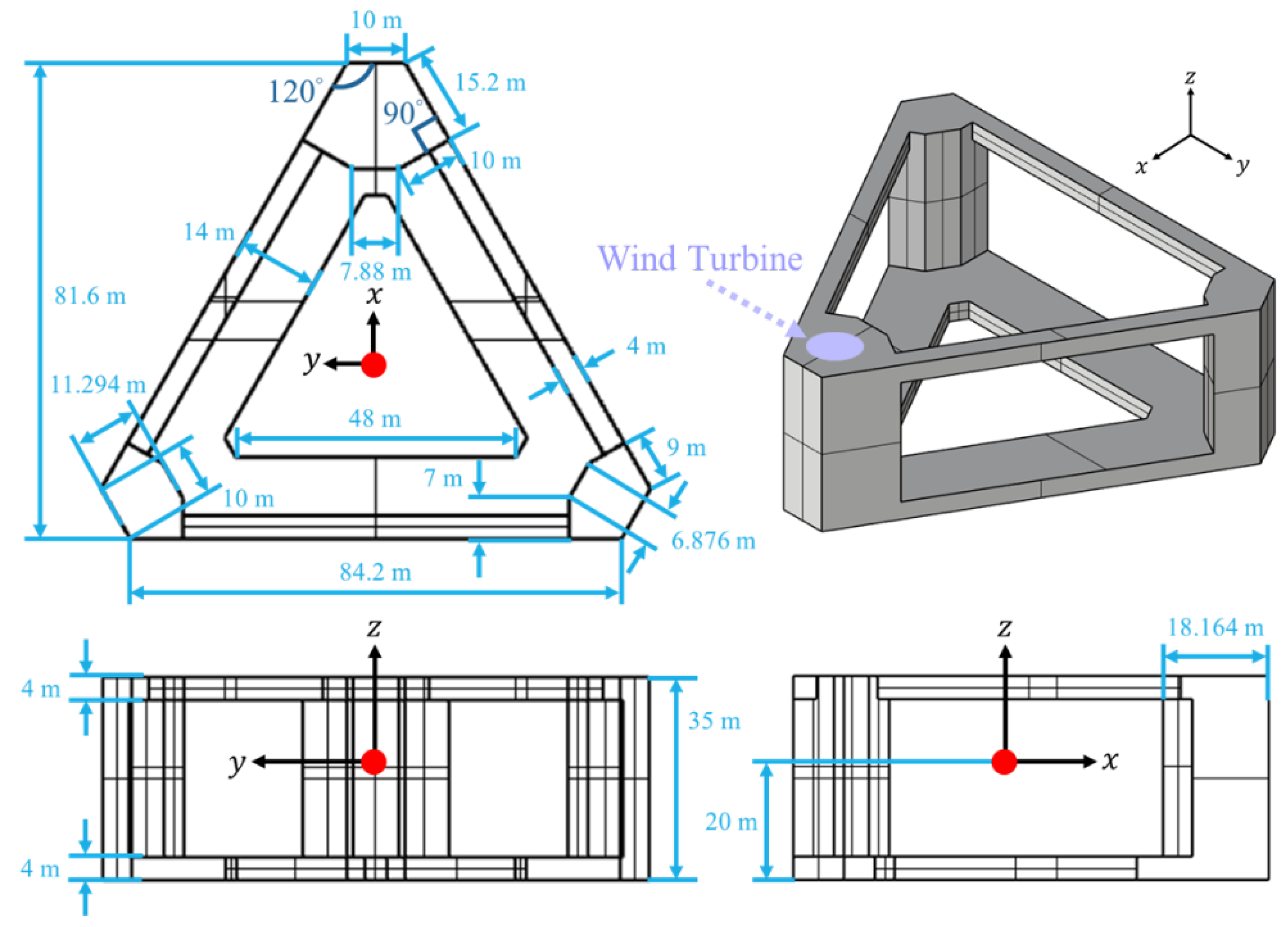
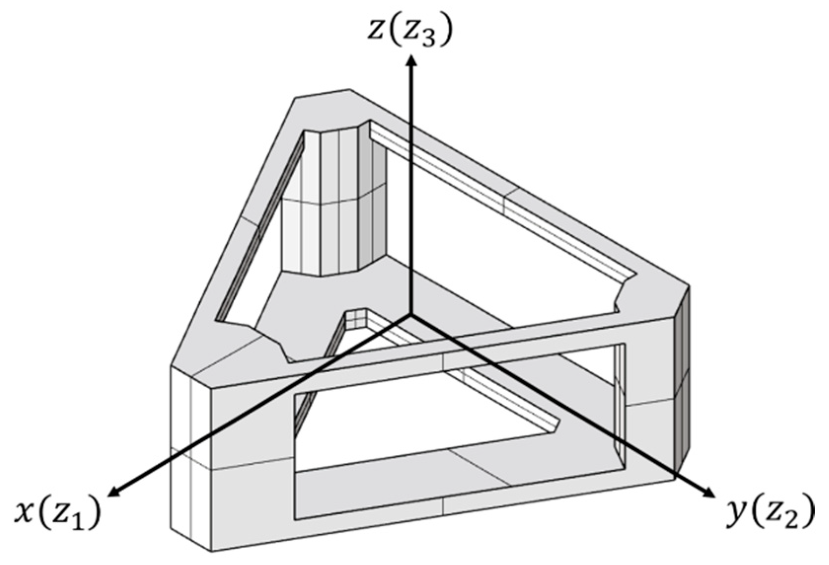
2.1. Floating Platform Design
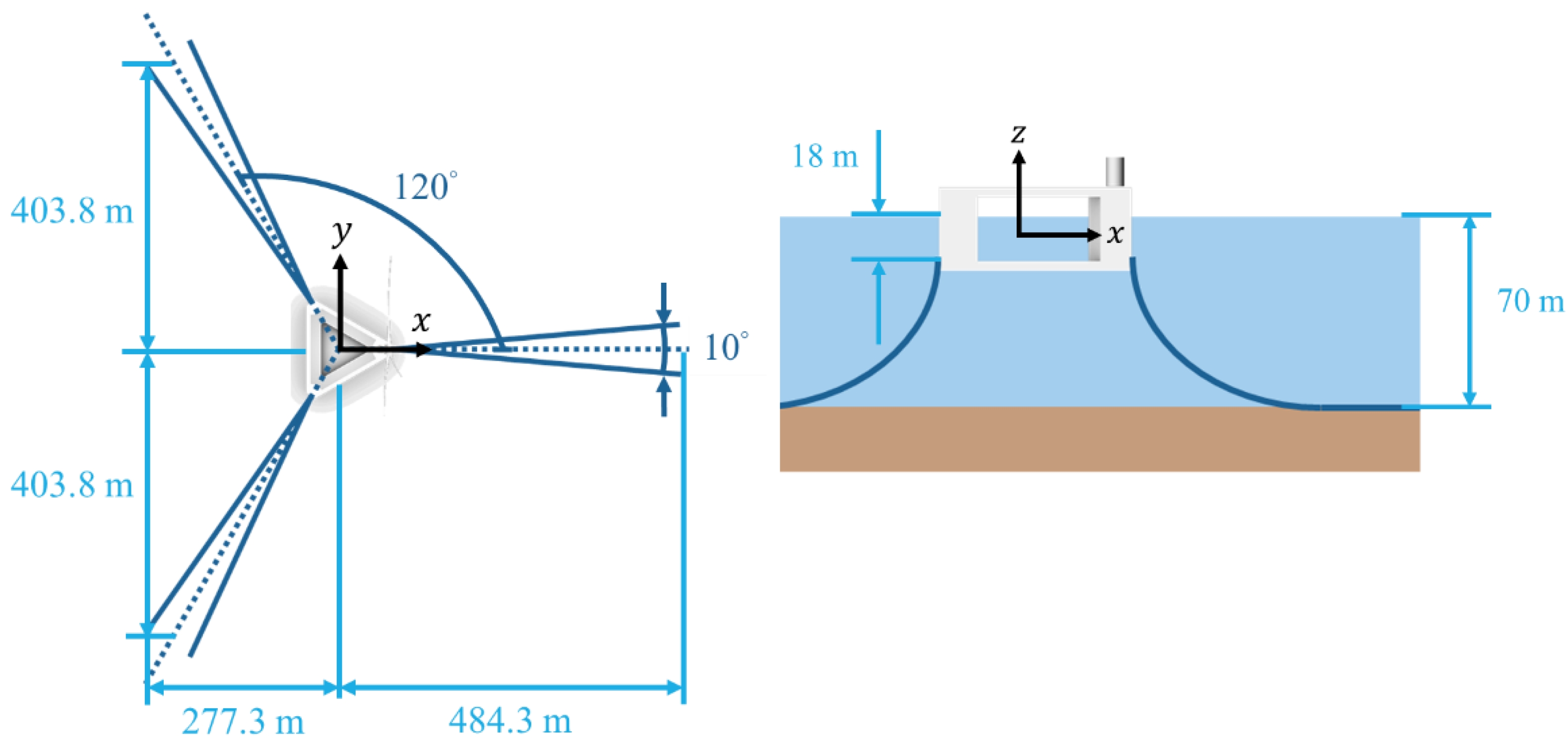
2.2. Mooring Design
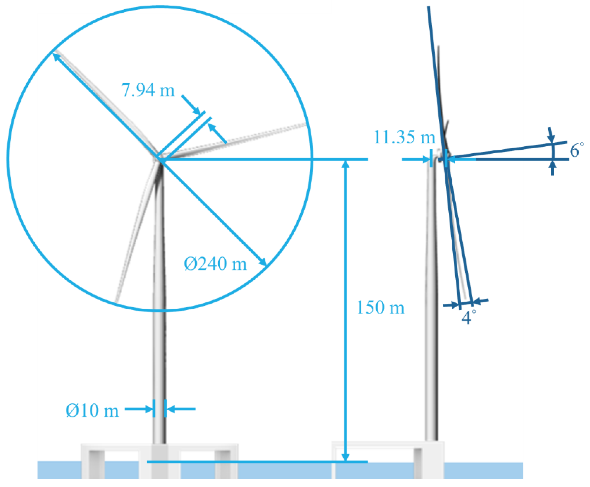
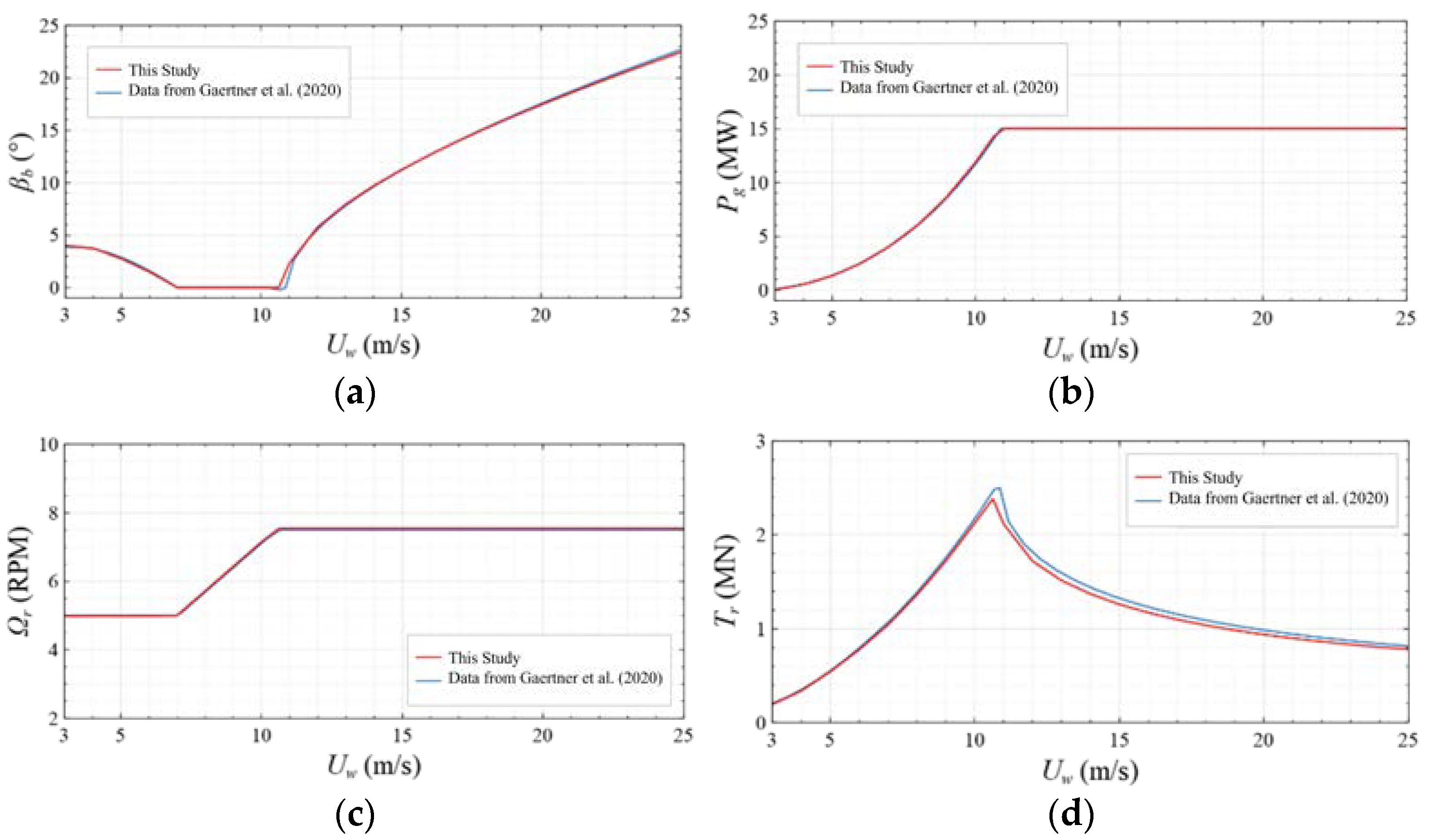
2.3. Wind Turbine Design
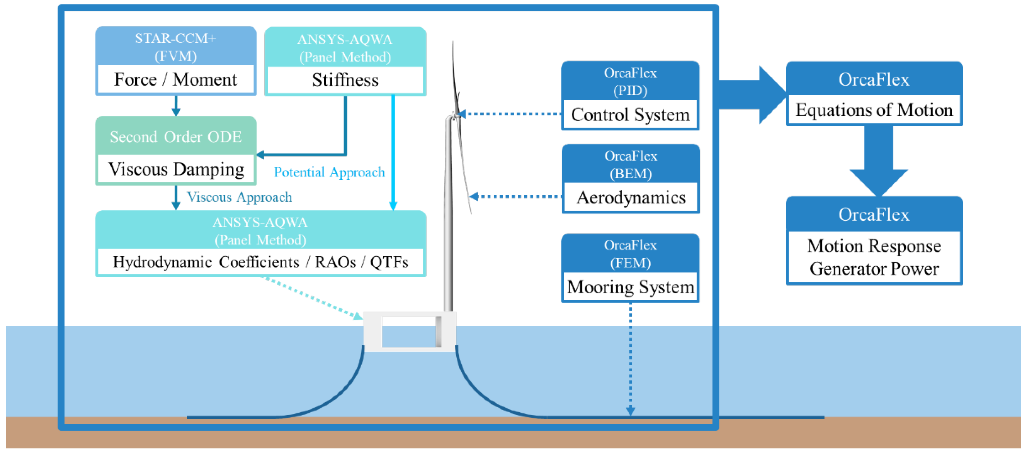
3. Numerical Methods
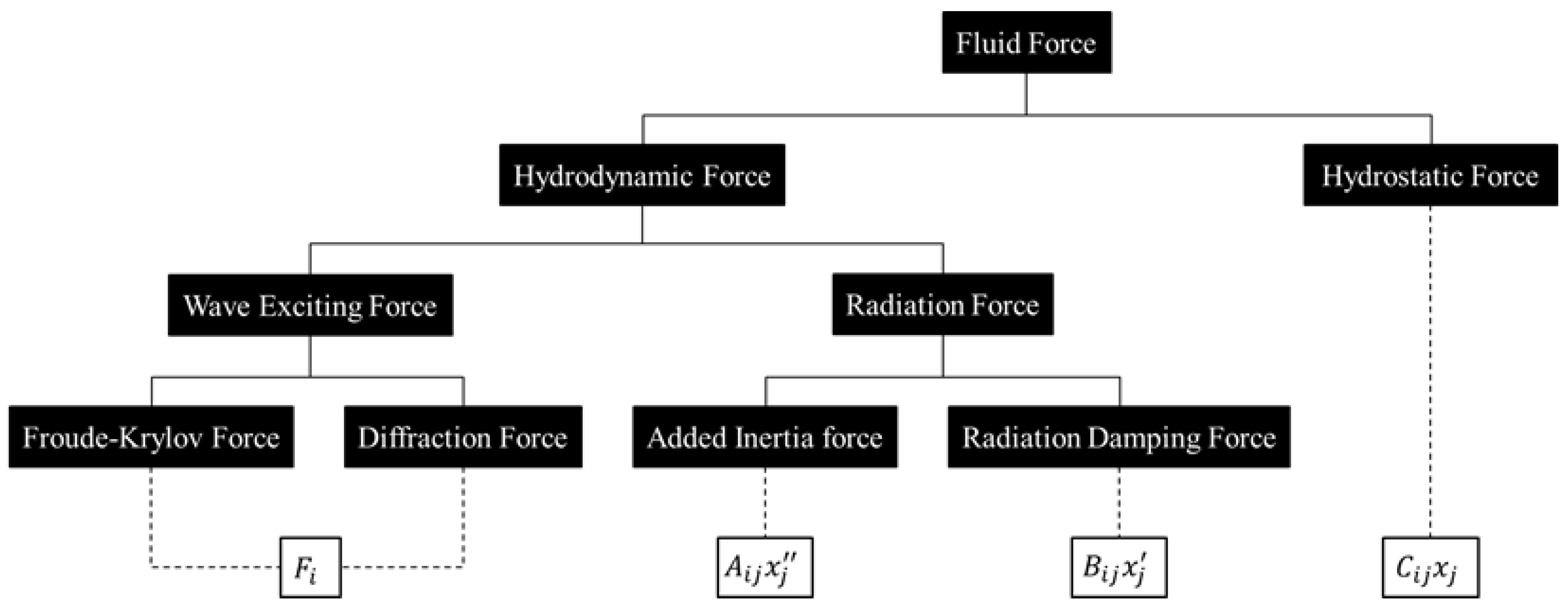
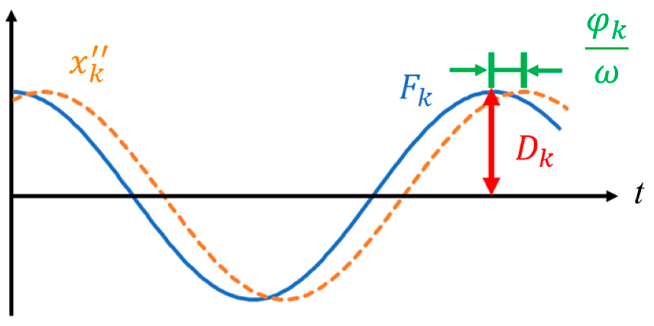
3.1. Equations of Motion
3.2. Potential-Flow Modeling
3.3. Viscous Damping
3.4. Modeling of Floating Wind Turbine System
3.4.1. Aerodynamic Modeling
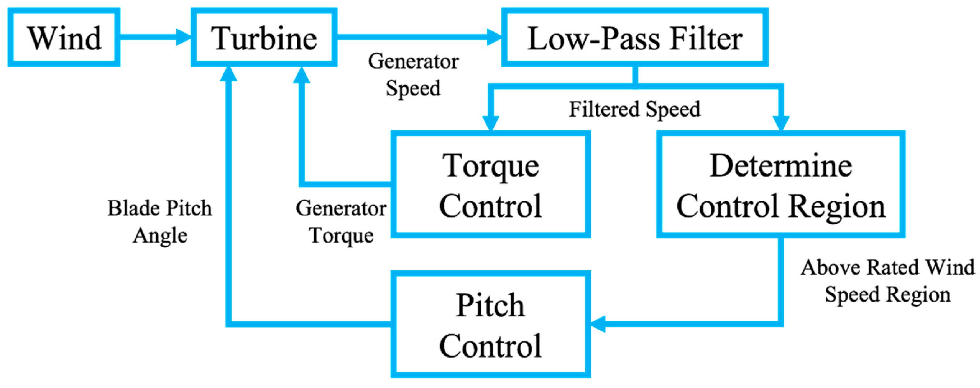
3.4.2. Control System Modeling
3.4.3. Mooring Modeling
4. Performance Prediction
4.1. Case Description
4.2. Hydrodynamic Properties
4.3. Motion Response and Generator Power
4.3.1. Common Wave Condition
4.3.2. High Wave Condition
4.4. Mooring Line Tension
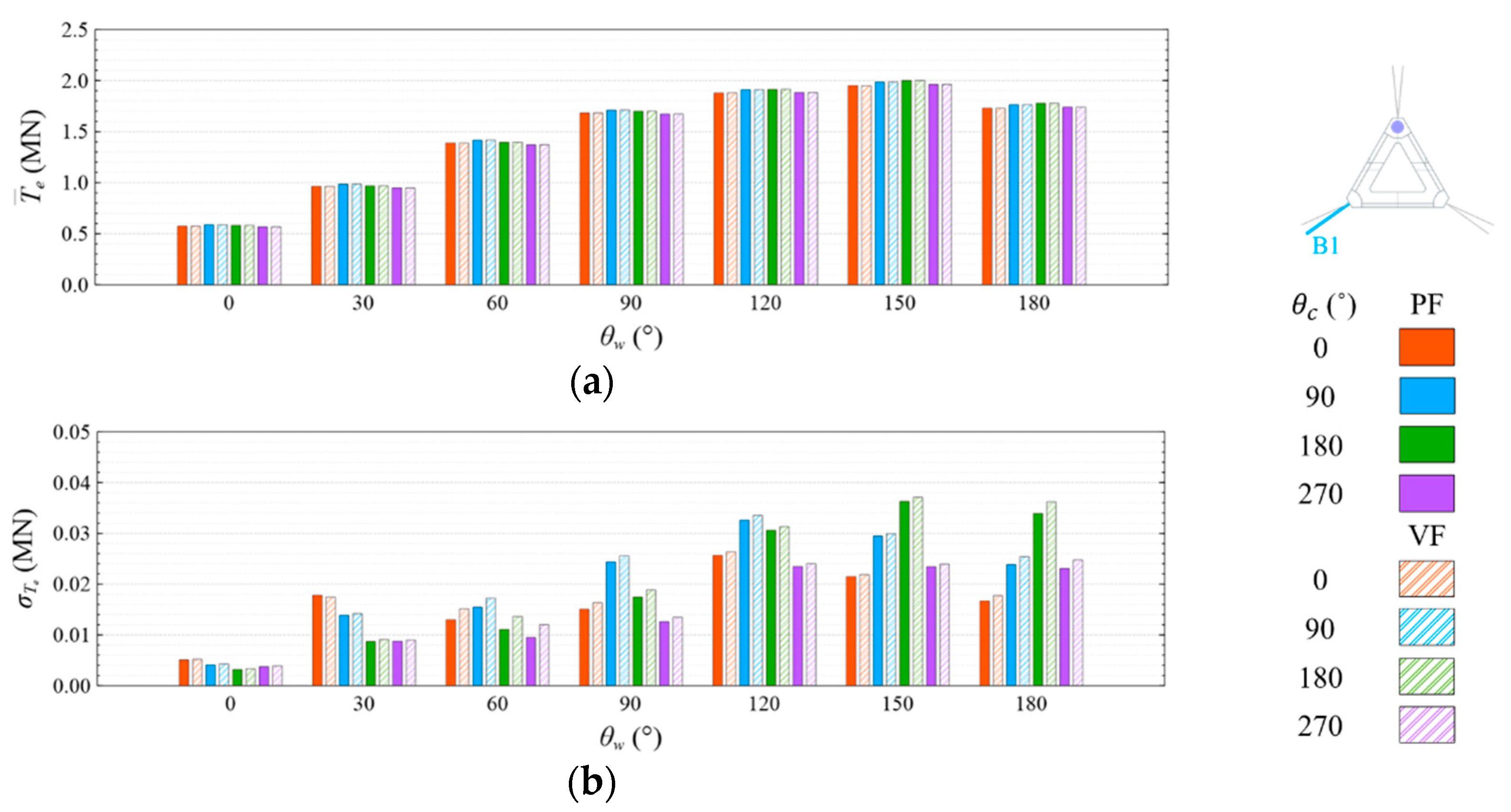
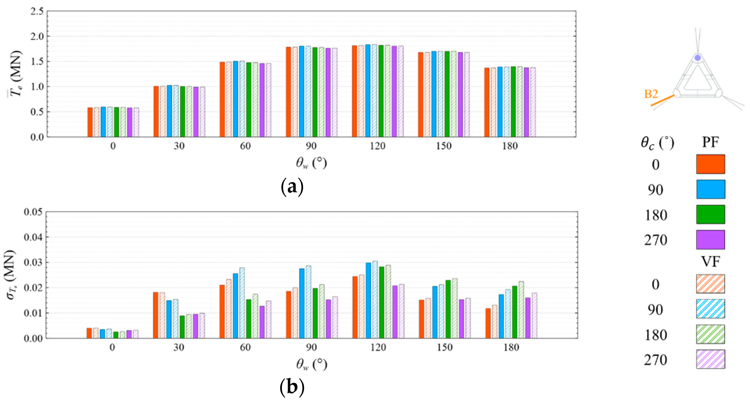
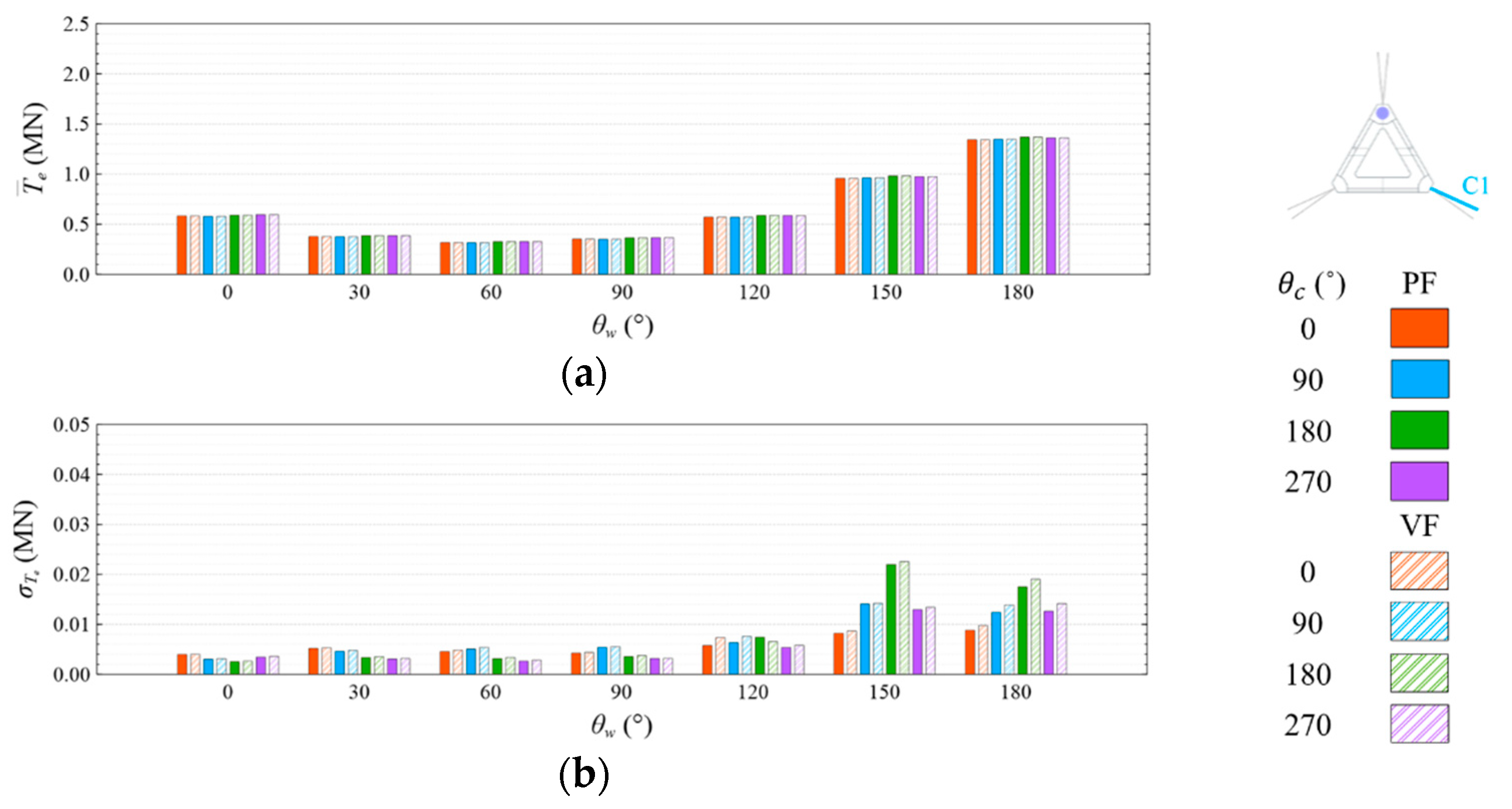
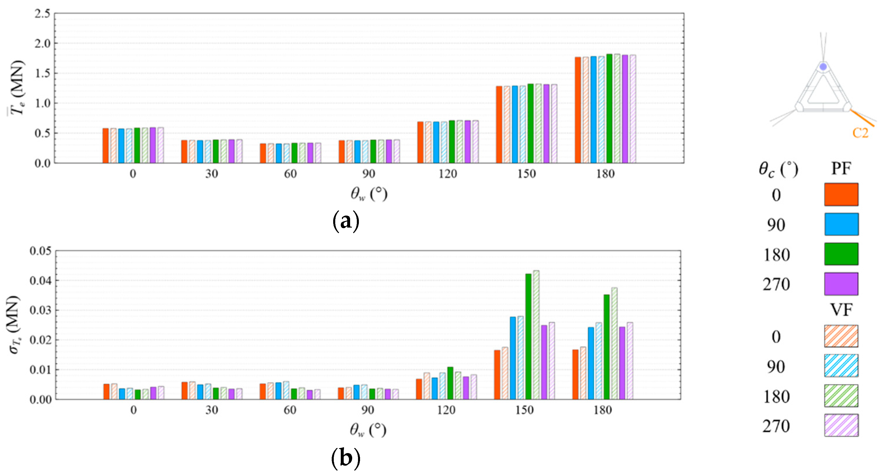
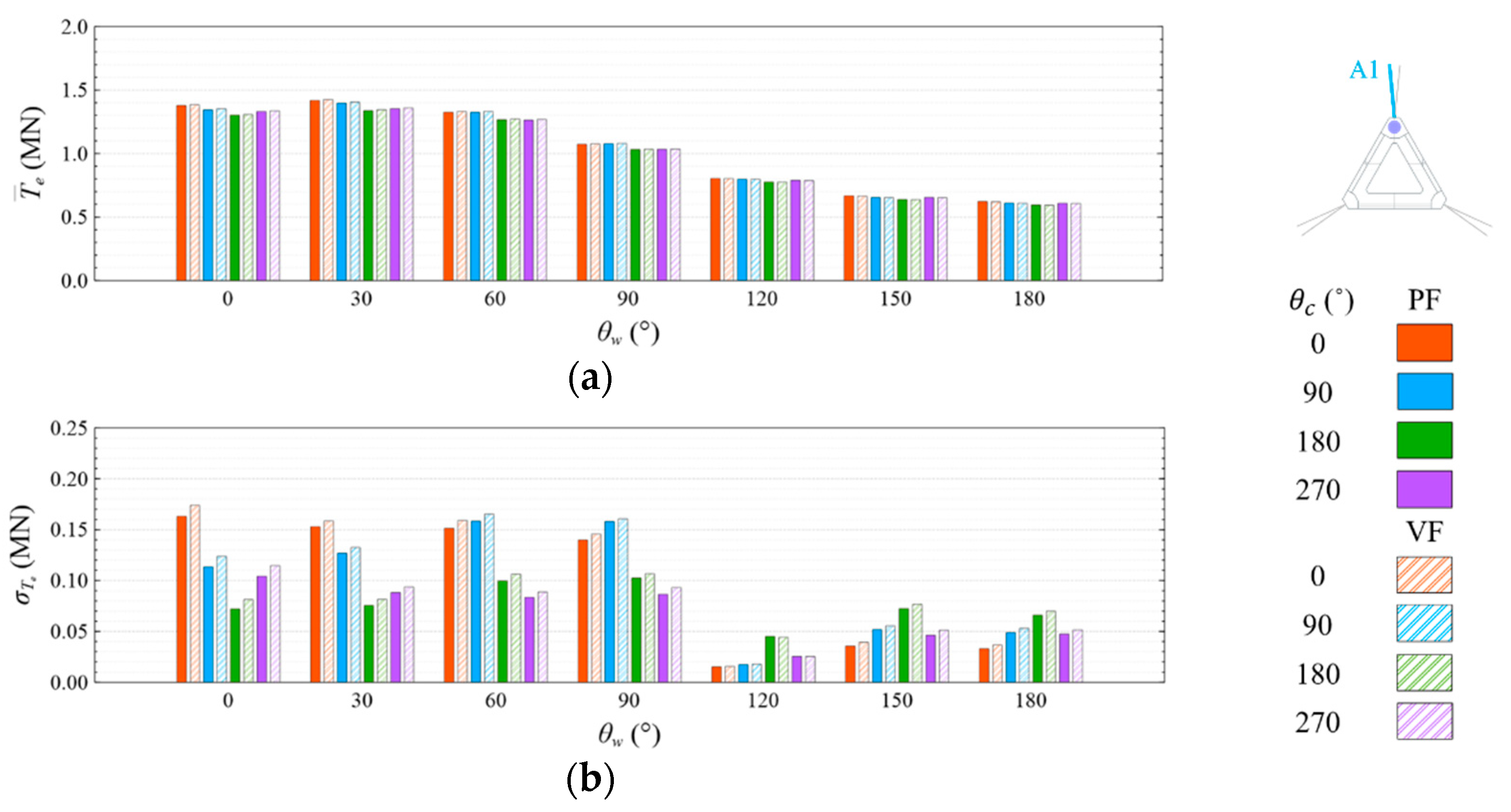
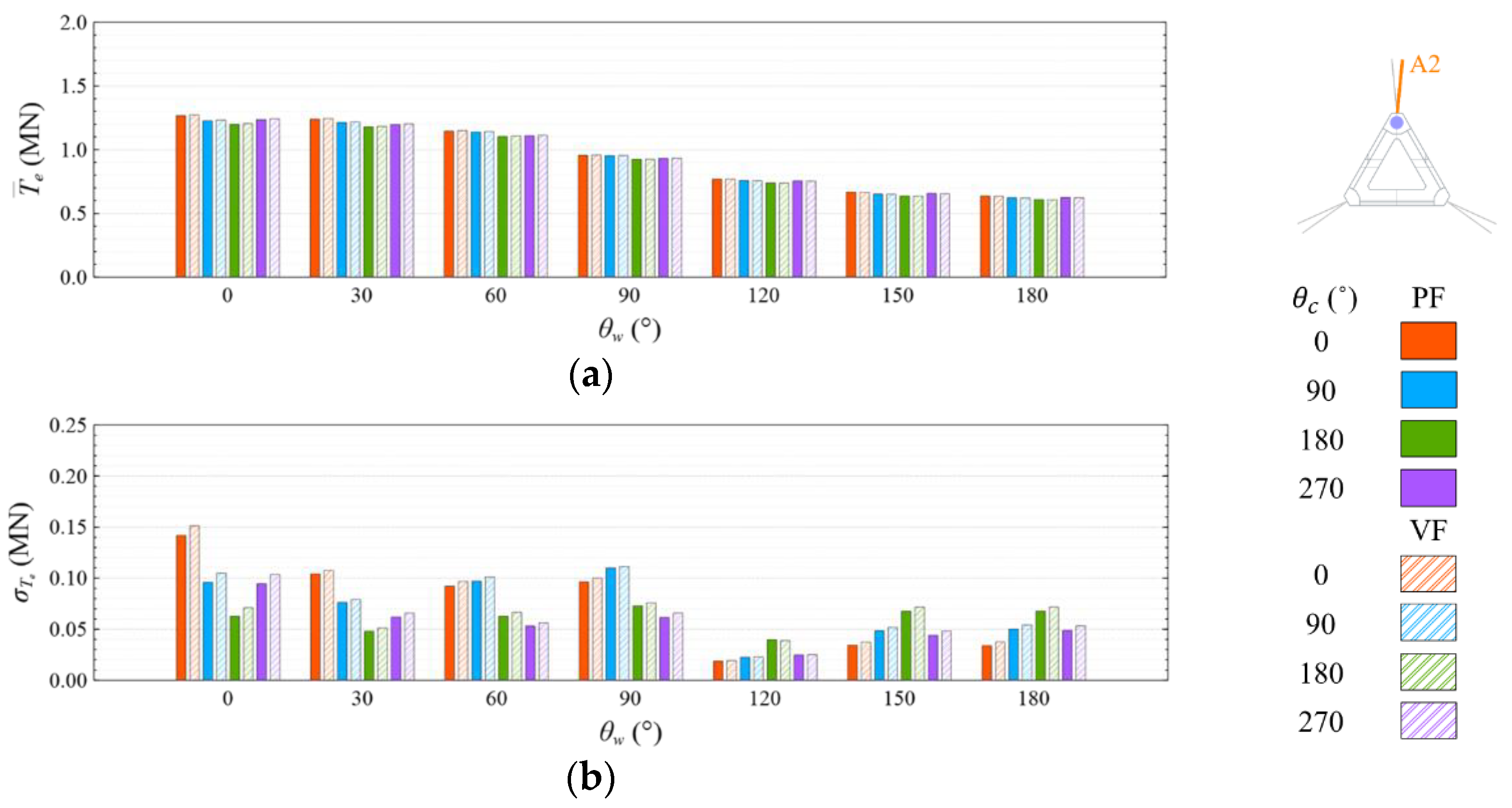
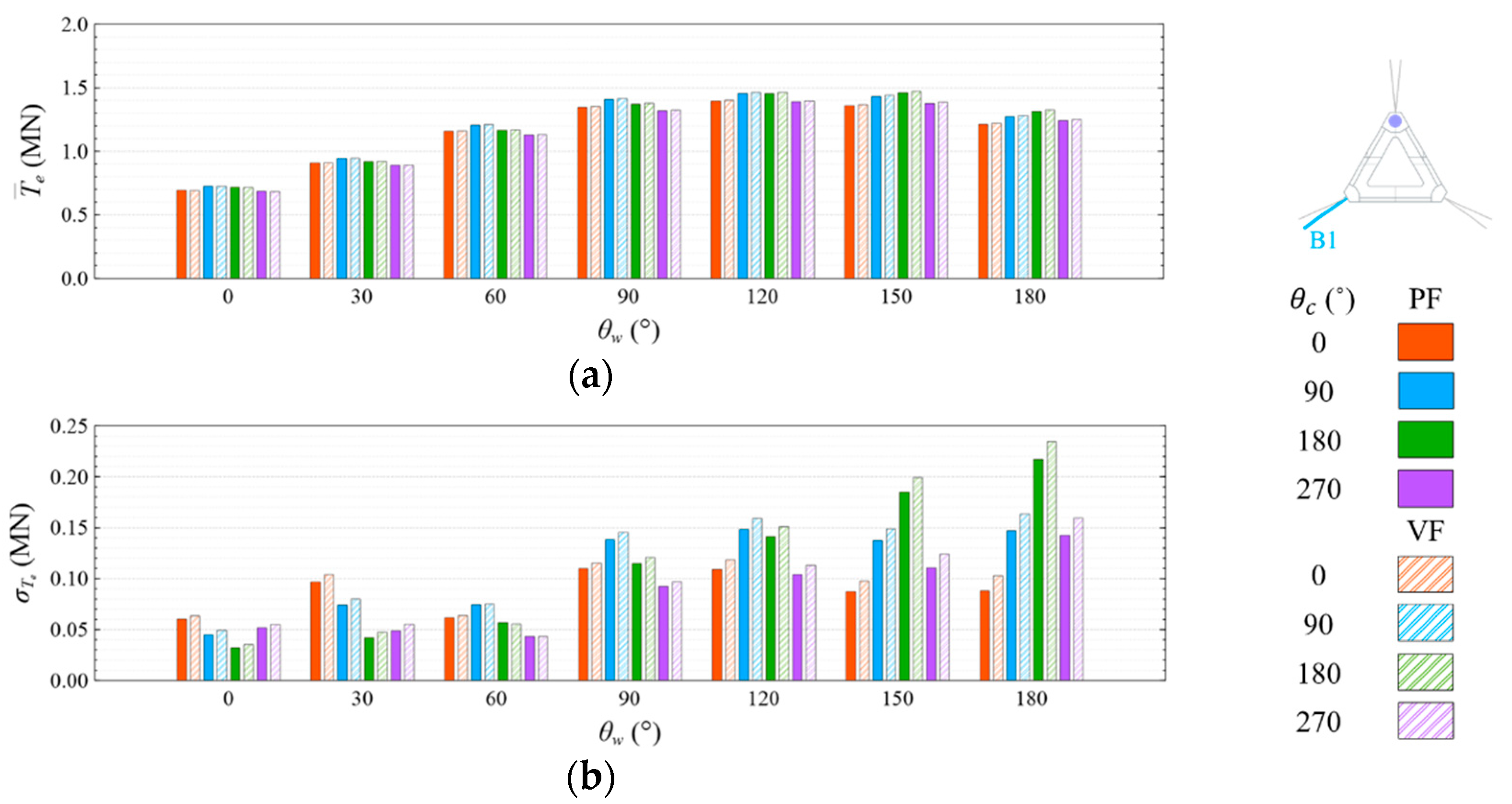
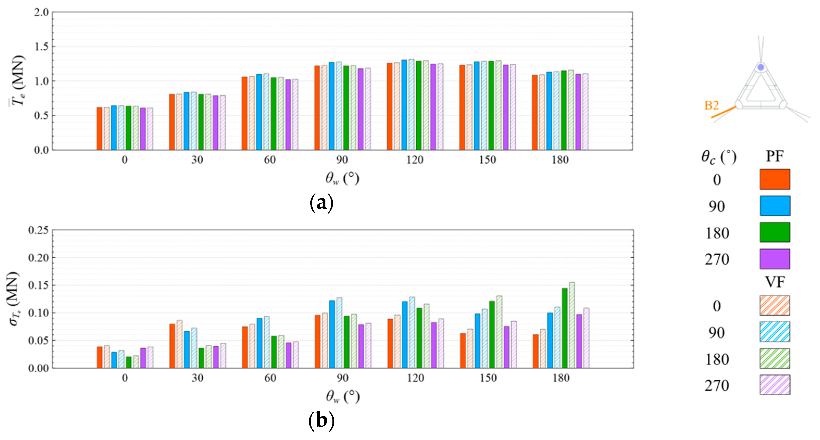
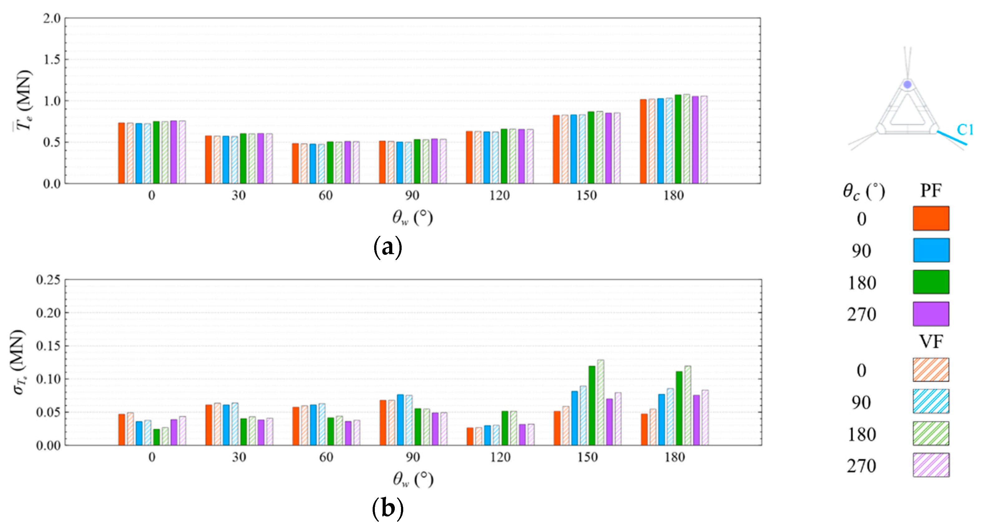
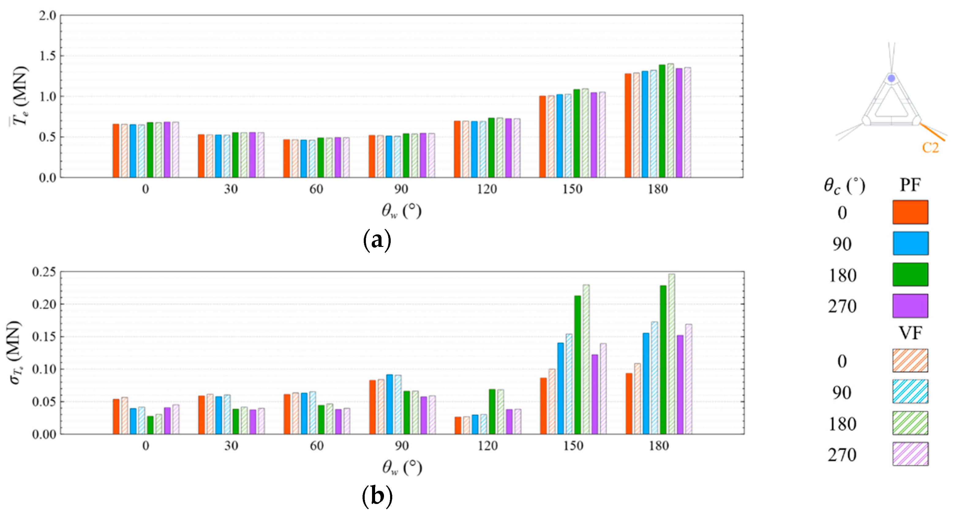
4.4.1. Common Wave Condition
4.4.2. High Wave Condition
5. Conclusions
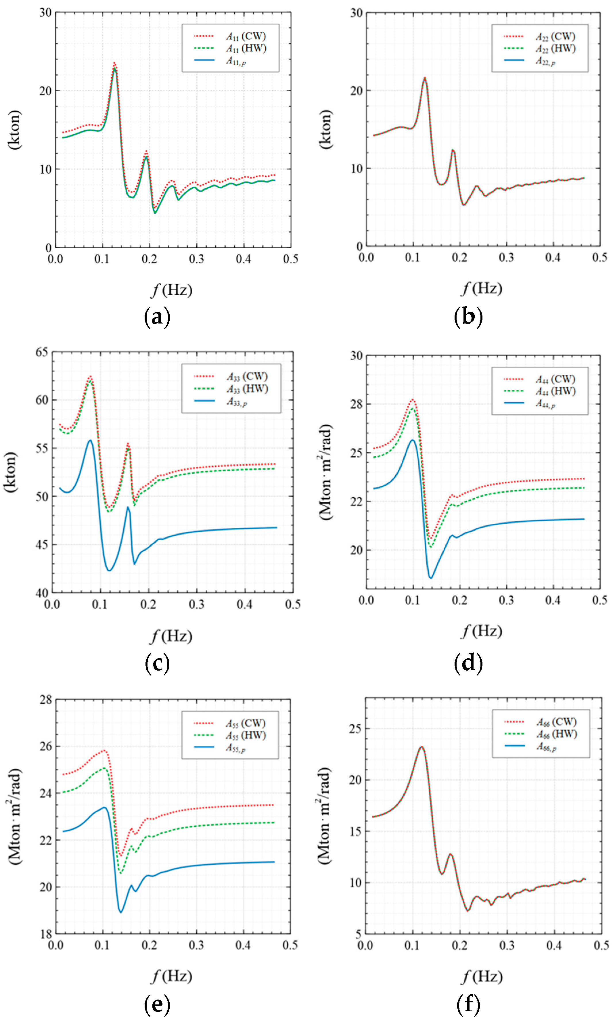
- The viscous effect has a more substantial impact on the hydrodynamic properties in the heave, roll, and pitch motions than in the surge, sway, and yaw motions. The viscous impact on the hydrodynamic properties under the CW condition is larger than that under the HW condition. The viscous prediction of the added mass in the heave motion increases by up to 15% of the potential result under the CW condition, while that in the heave motion under the HW condition increases by up to 14%. The viscous damping prediction in the roll motion increases by up to 13 times the potential result under the CW condition, while that in the heave motion under the HW condition increases by up to 6 times;
- The viscous effect has a more substantial impact on the hydrodynamic properties in the heave, roll, and pitch motions than in the surge, sway, and yaw motions. The viscous impact on the hydrodynamic properties under the CW condition is larger than that under the HW condition;
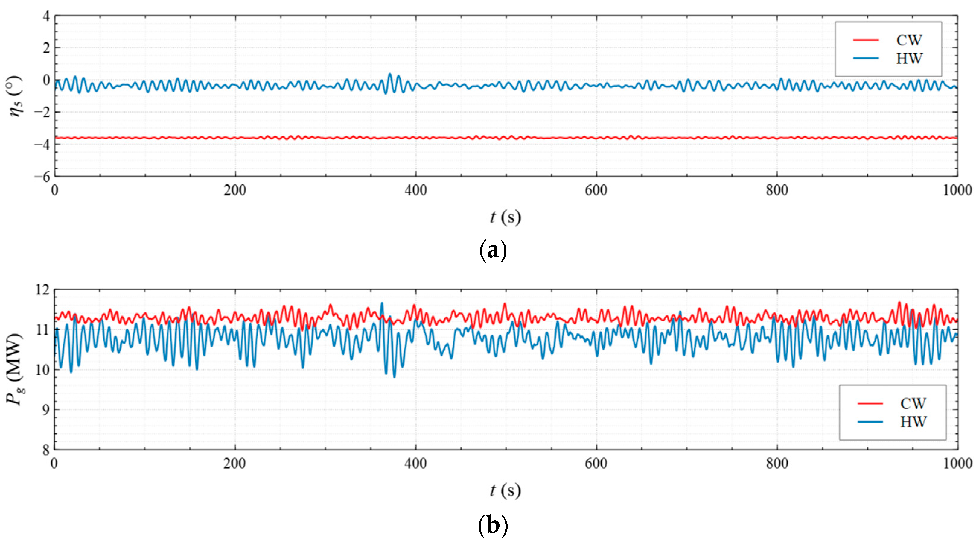
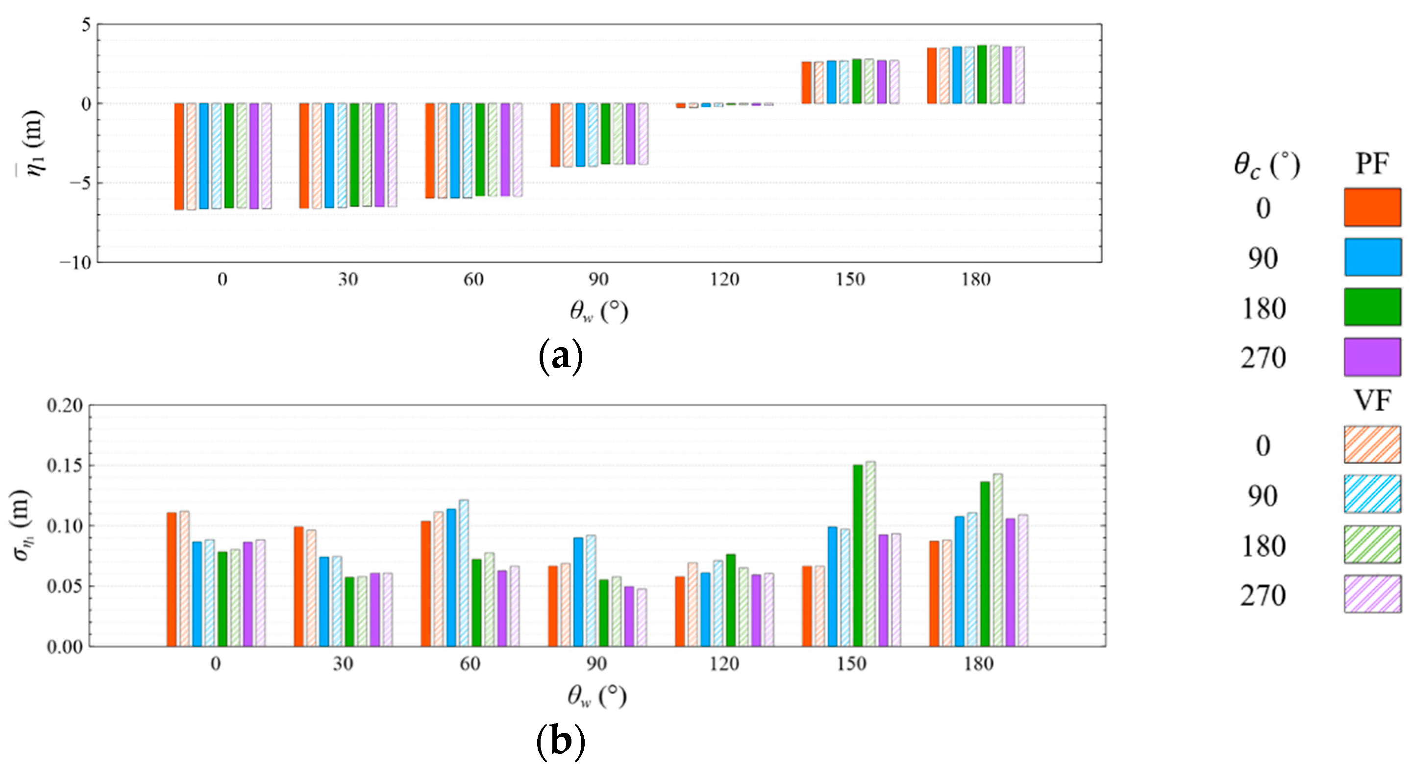
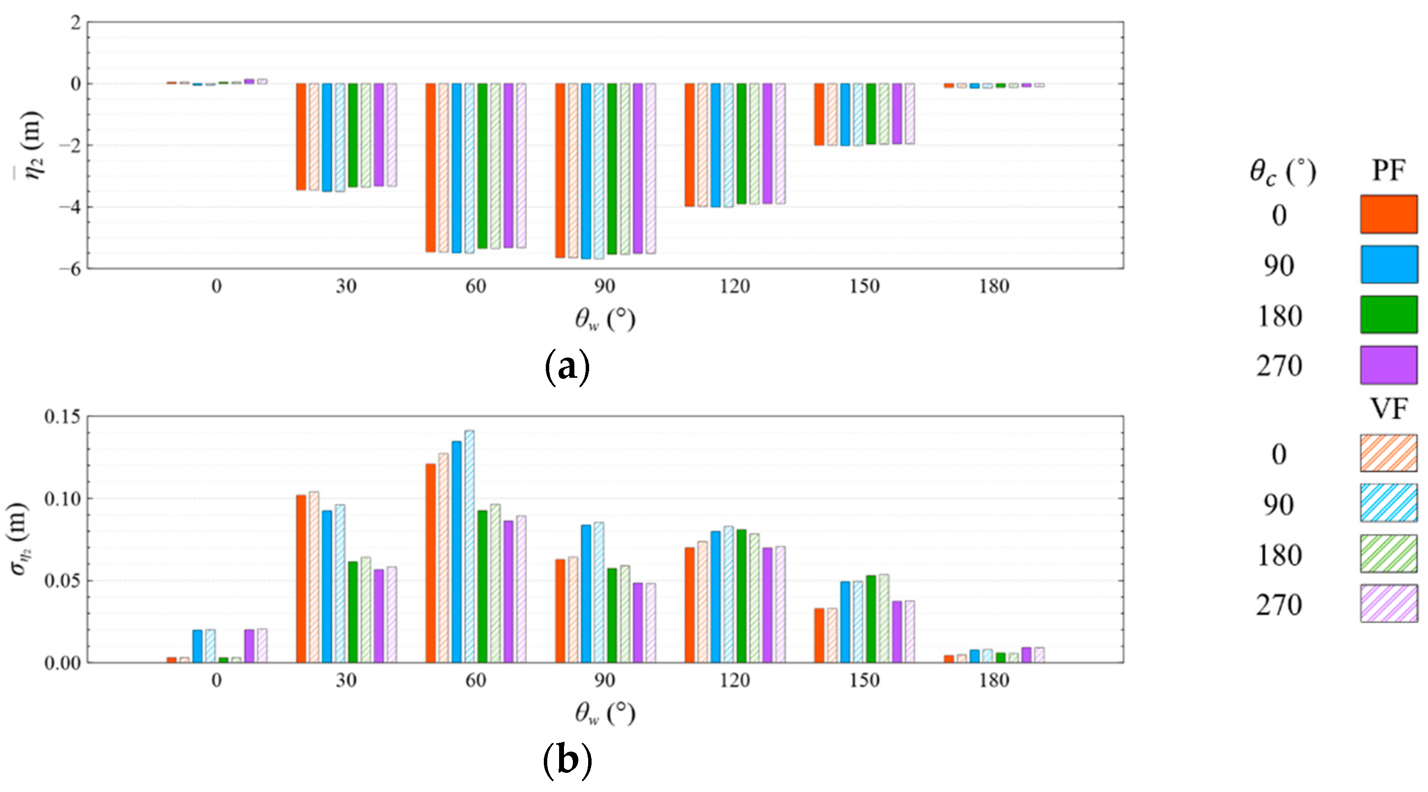
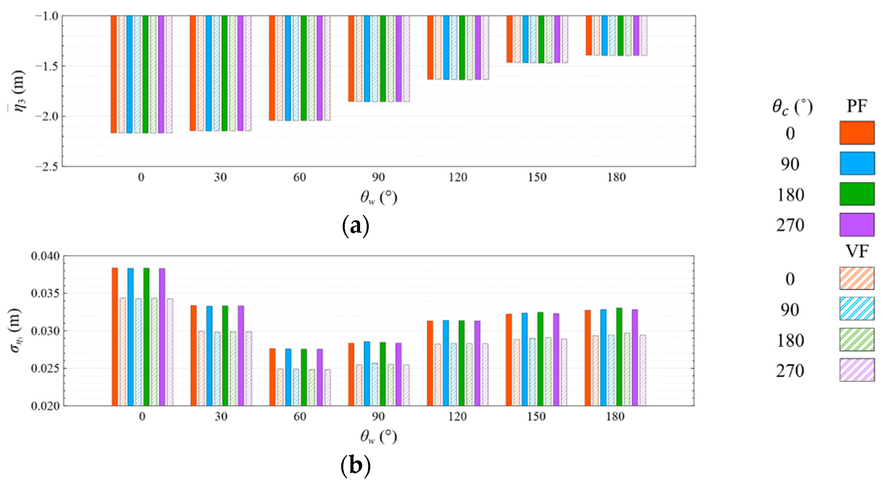
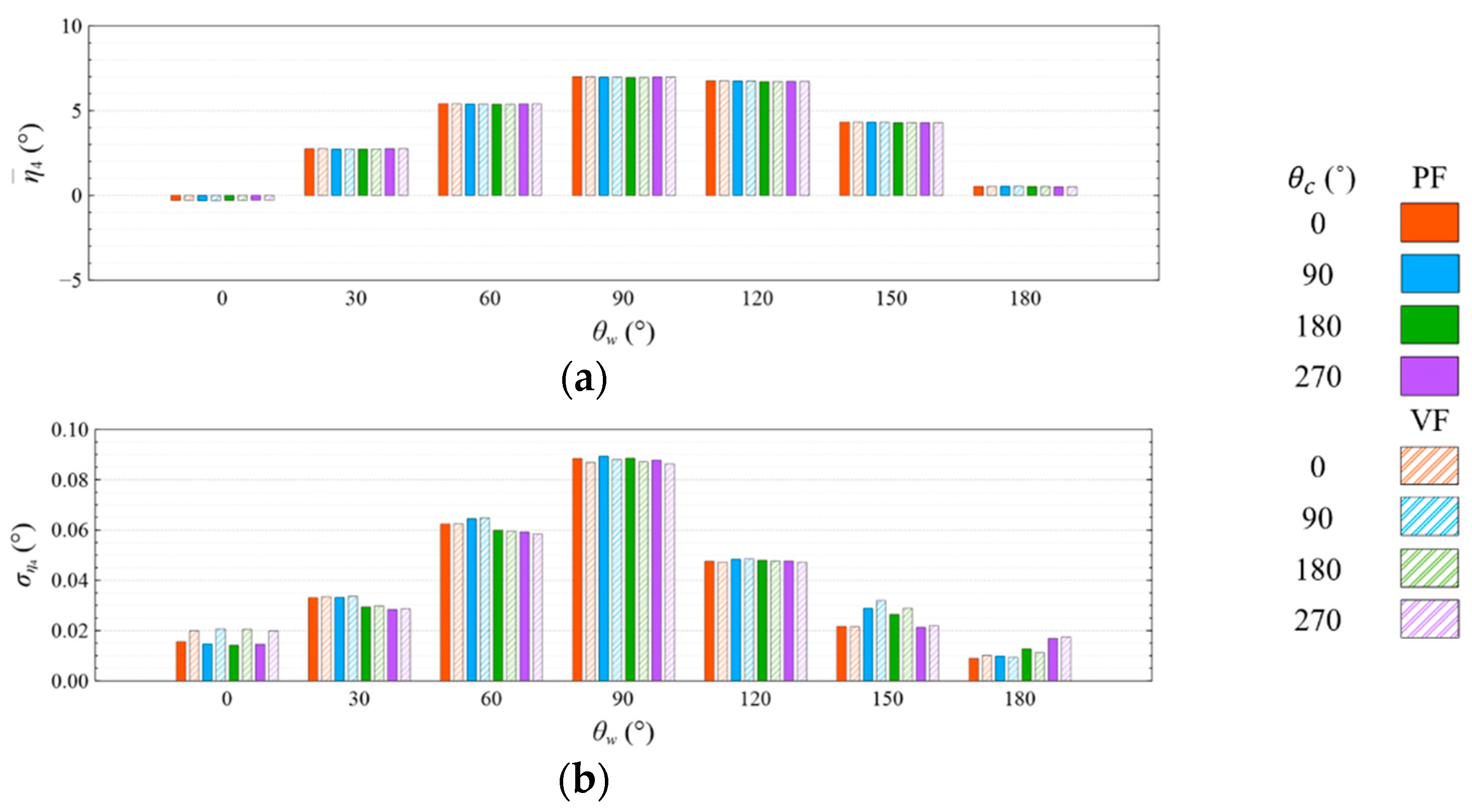
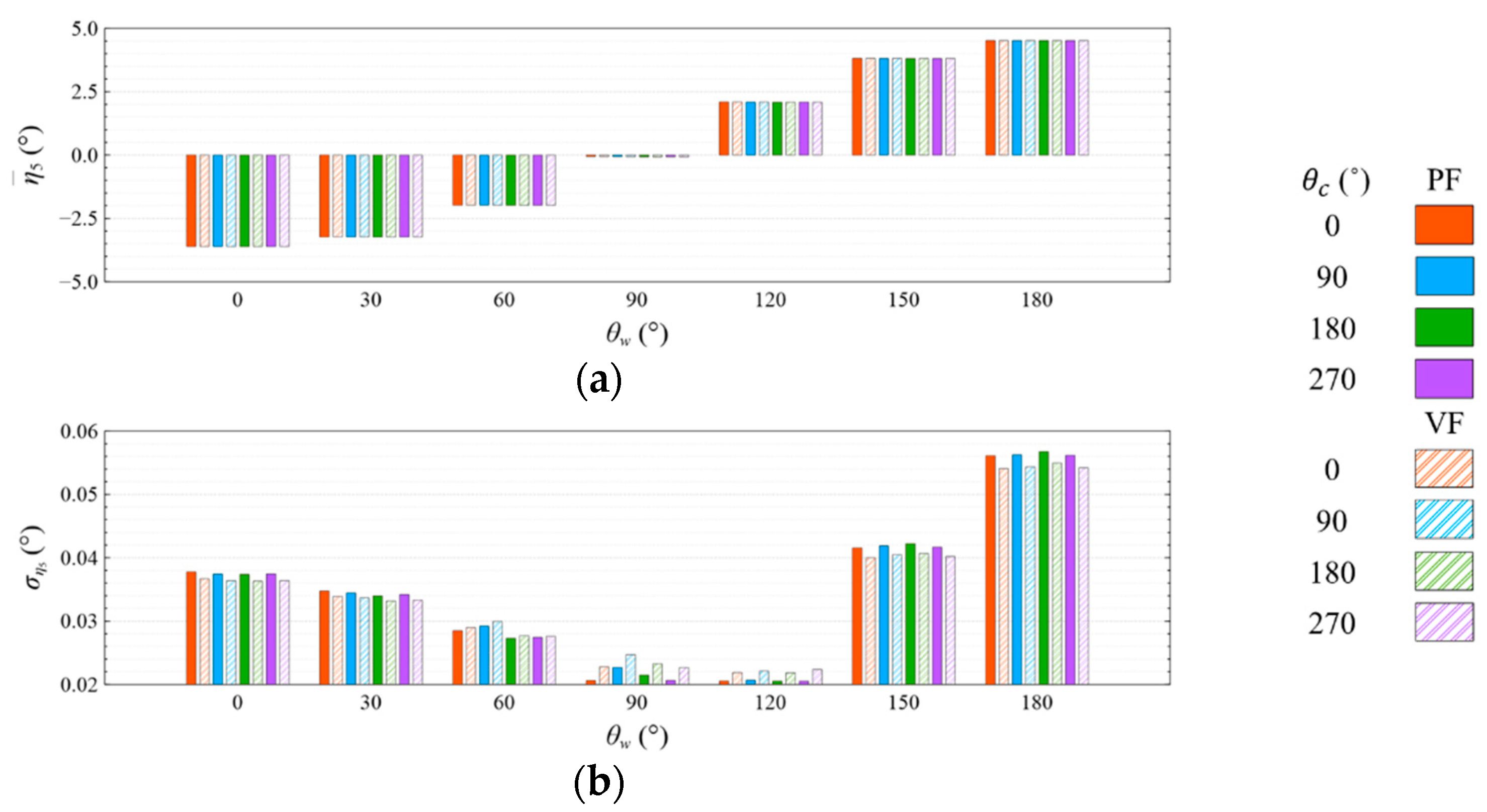
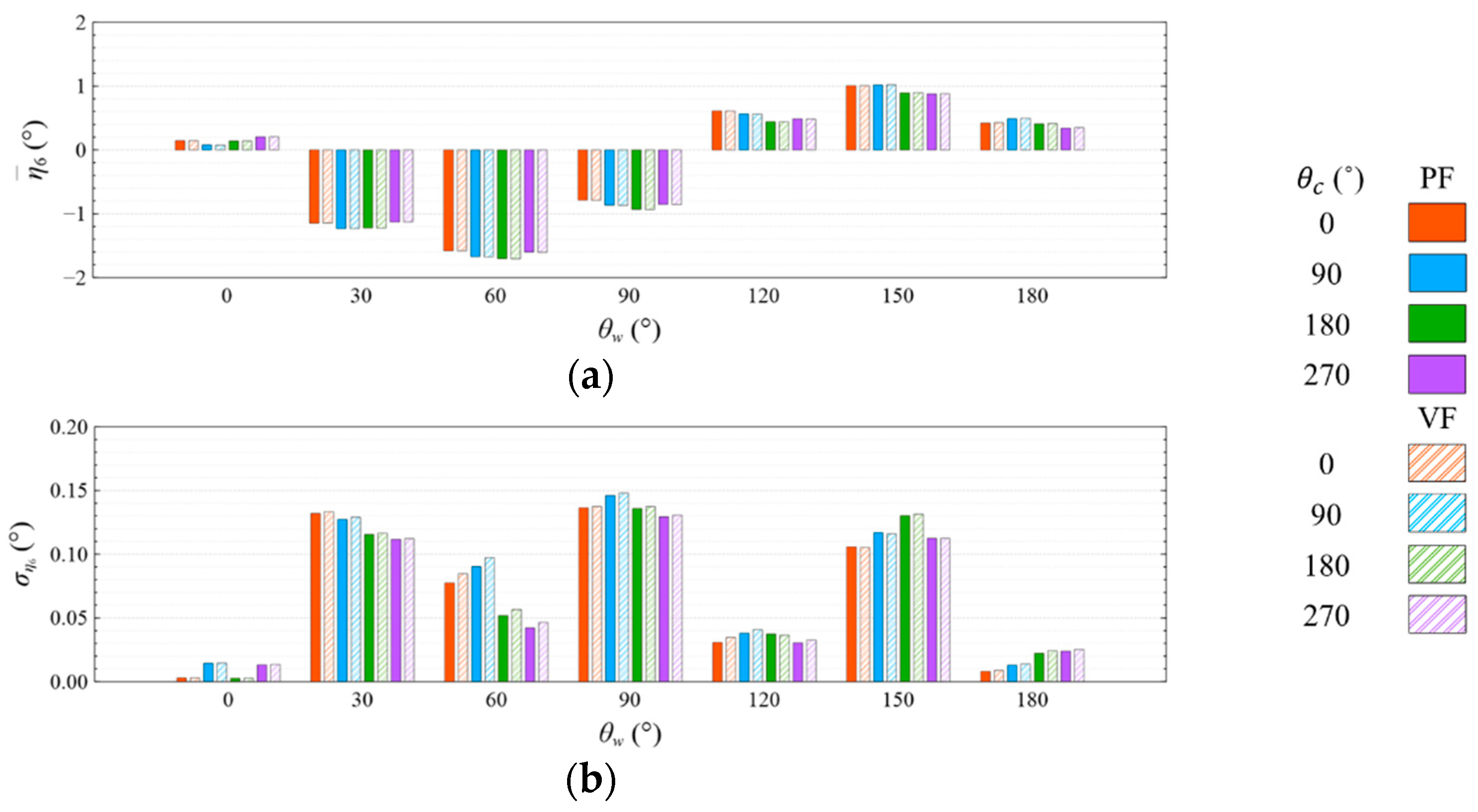
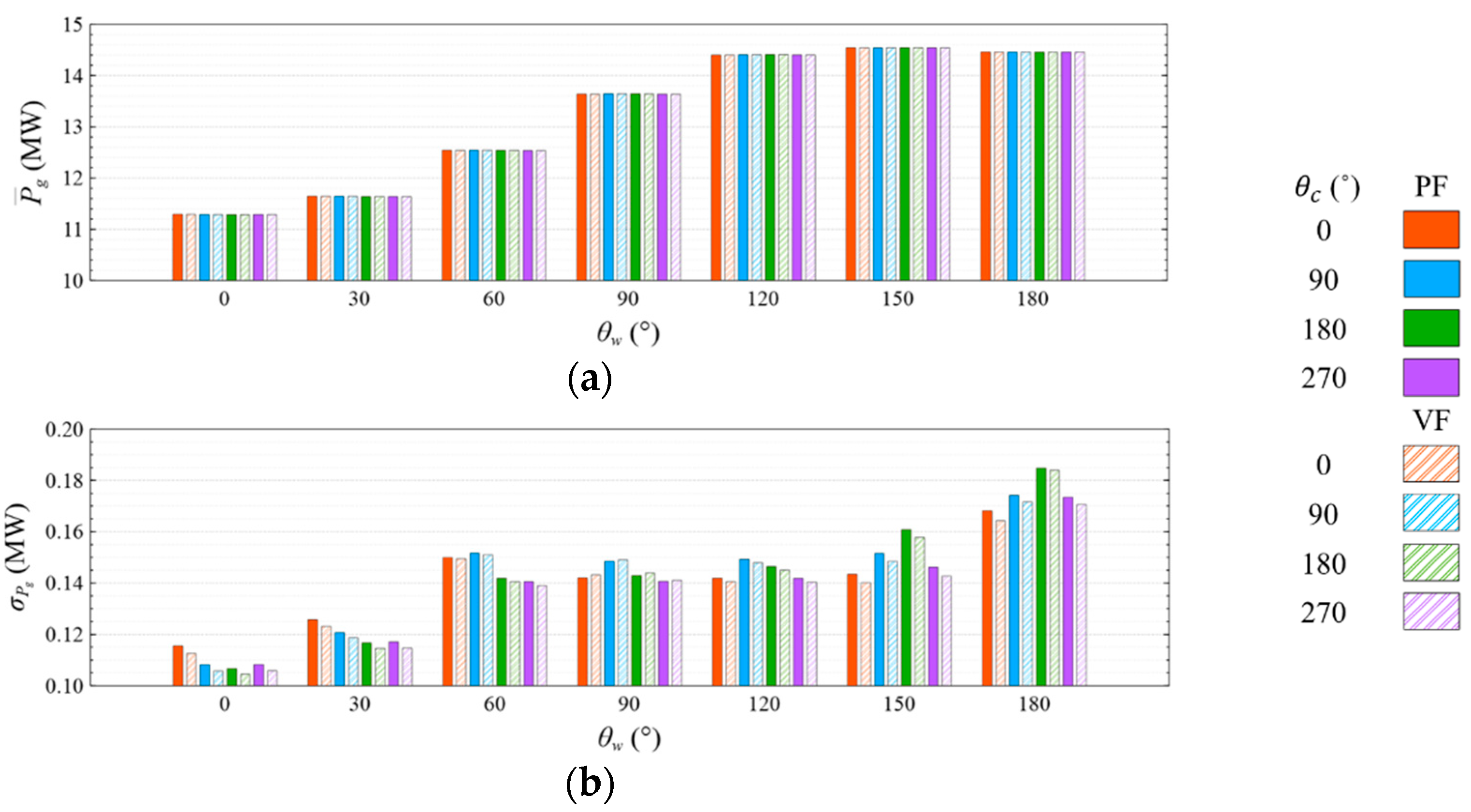
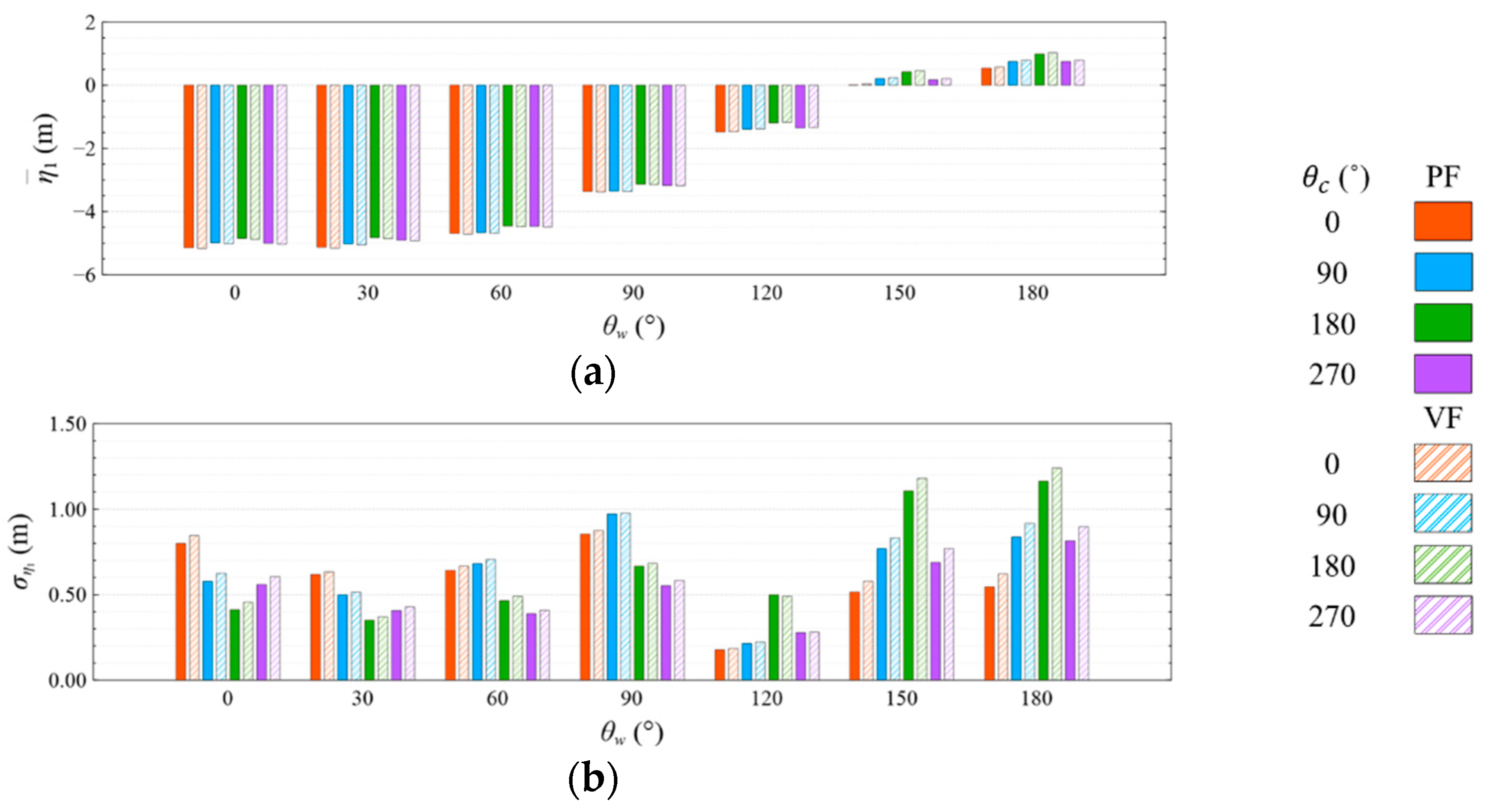
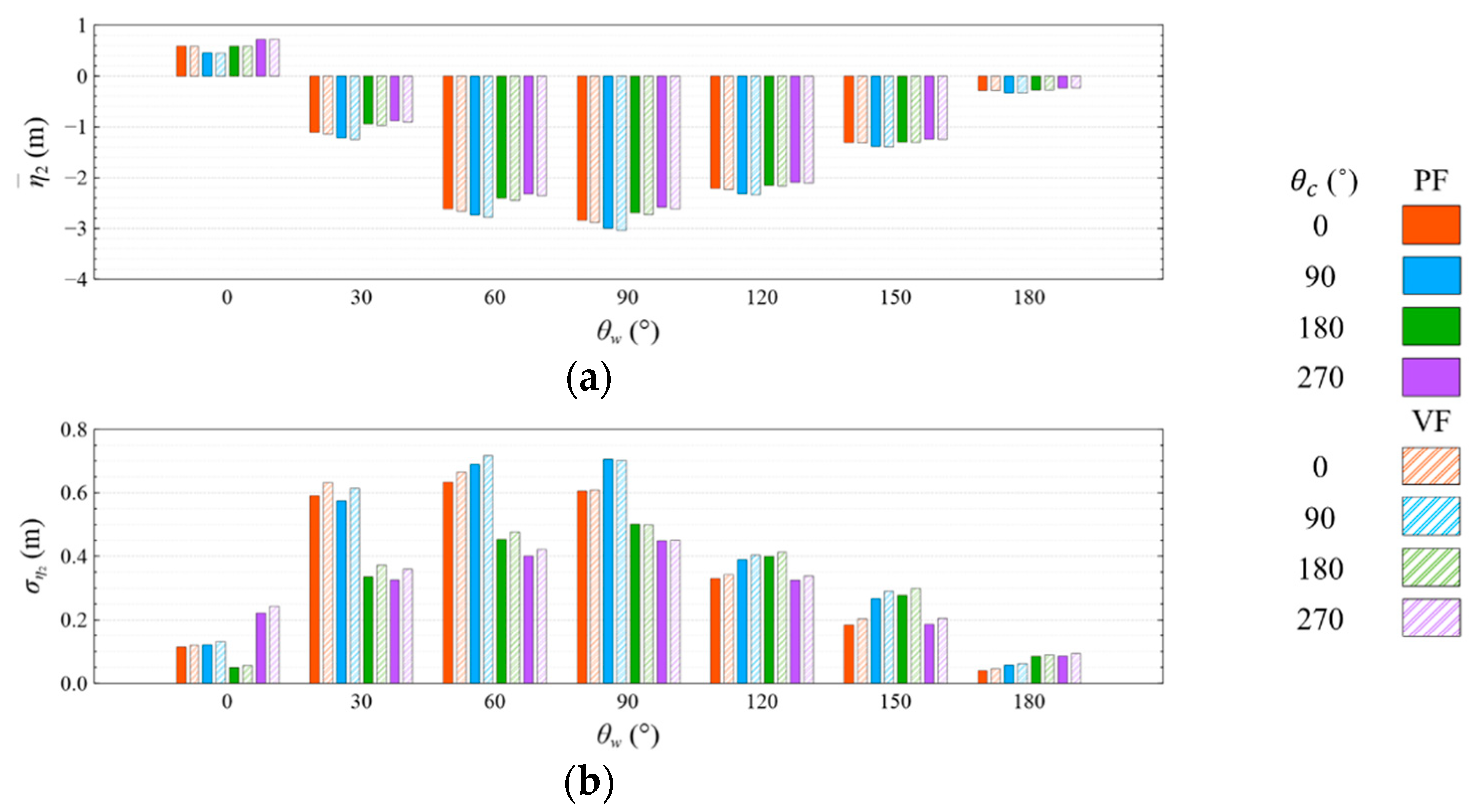
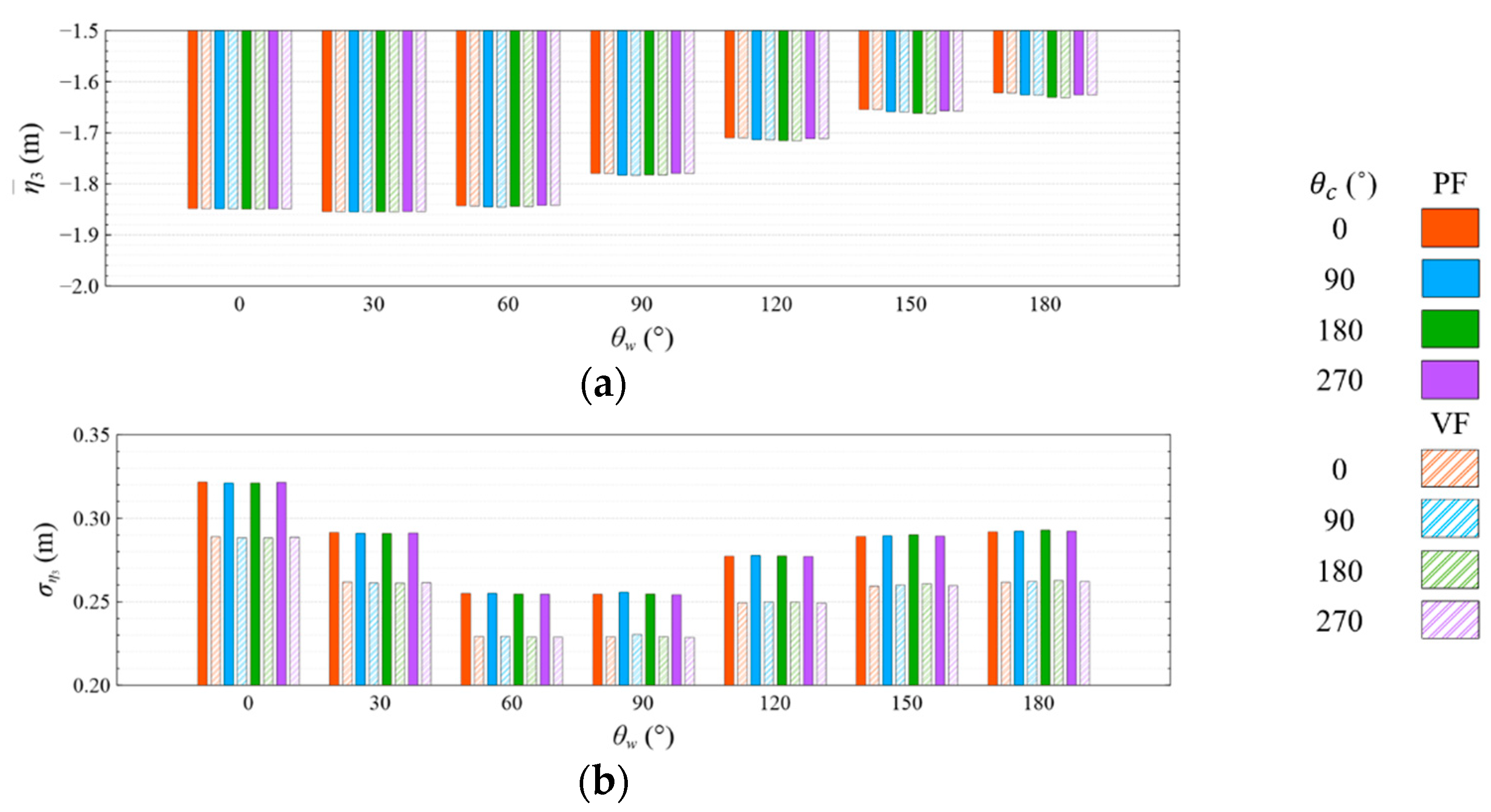
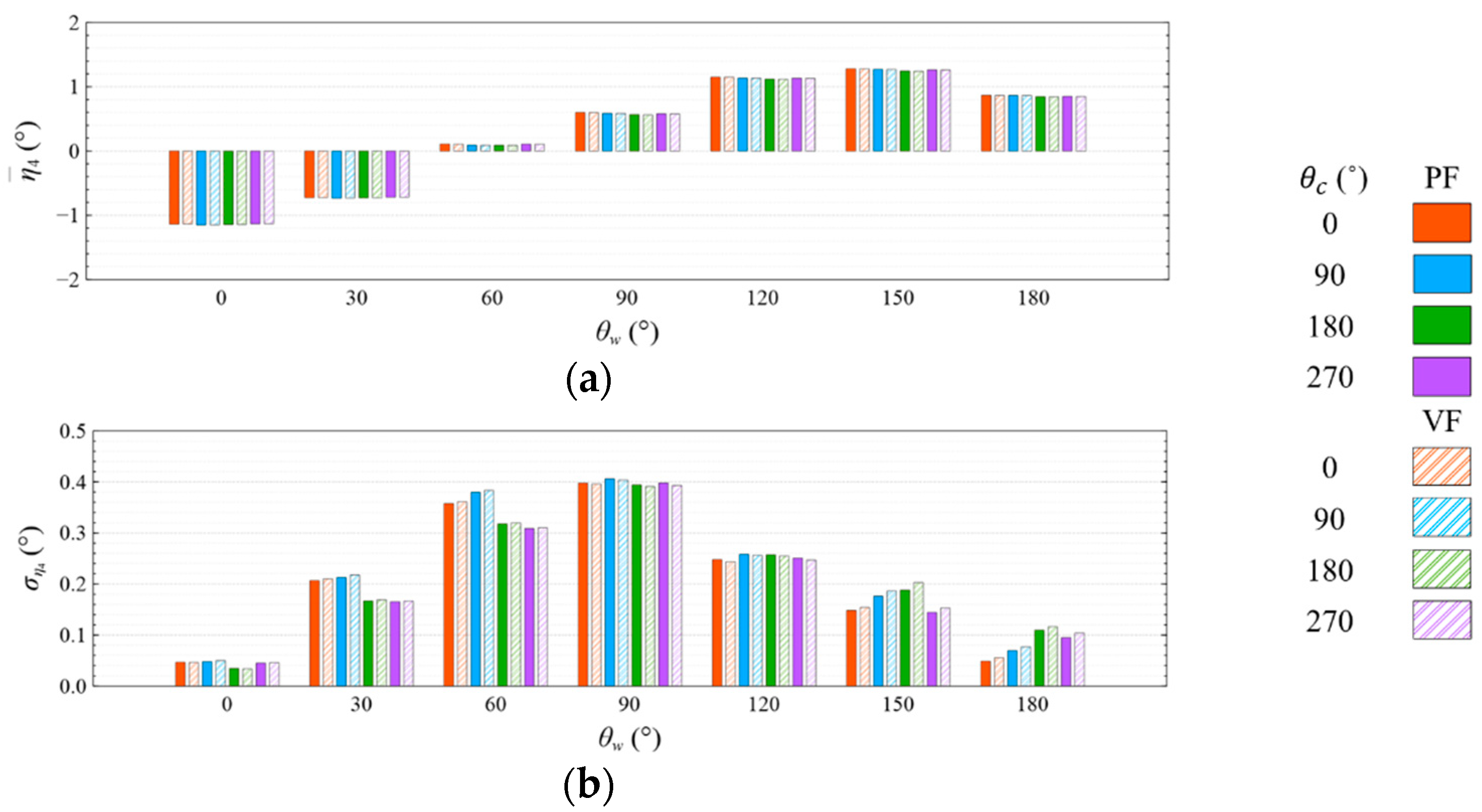
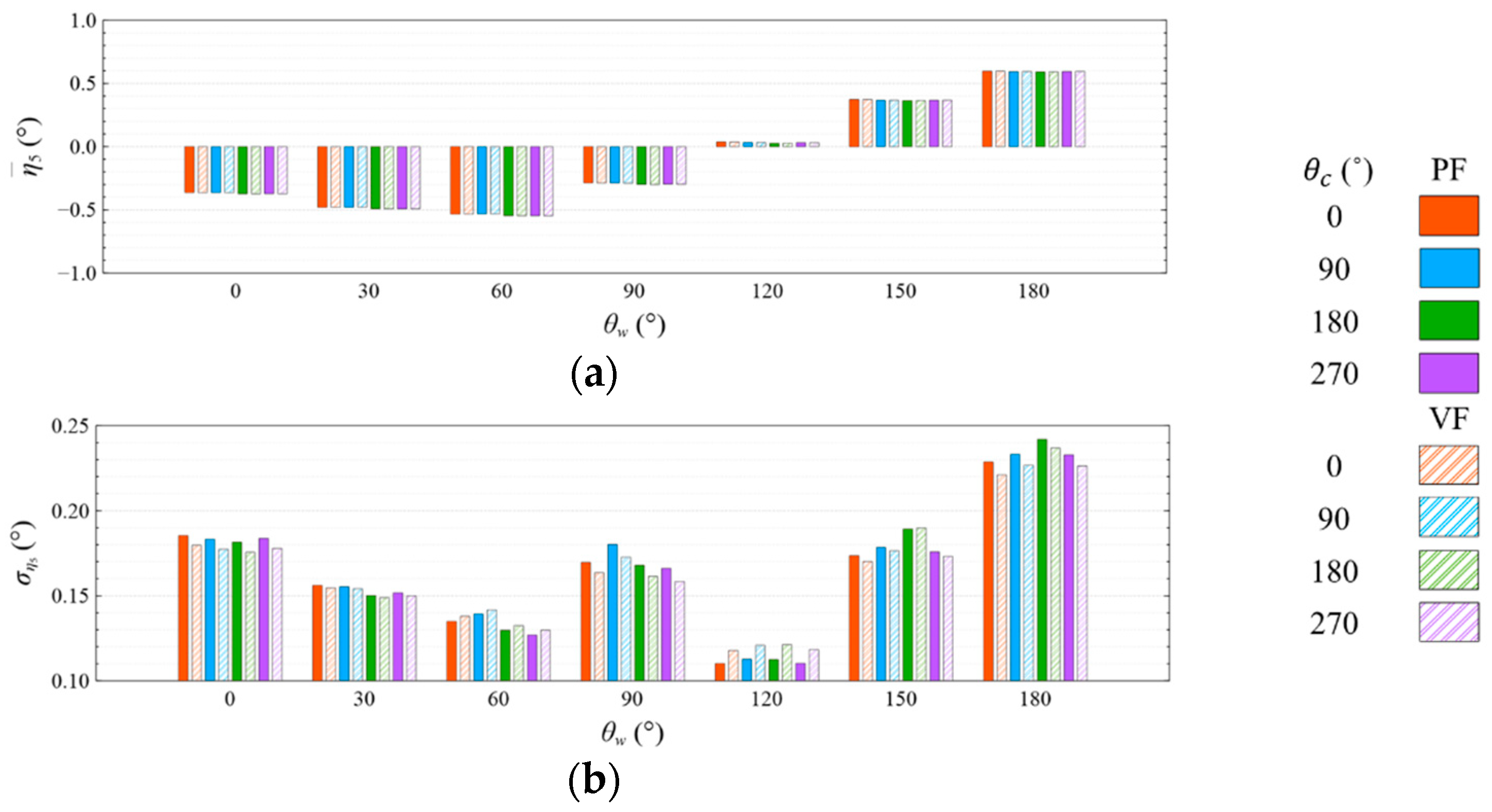
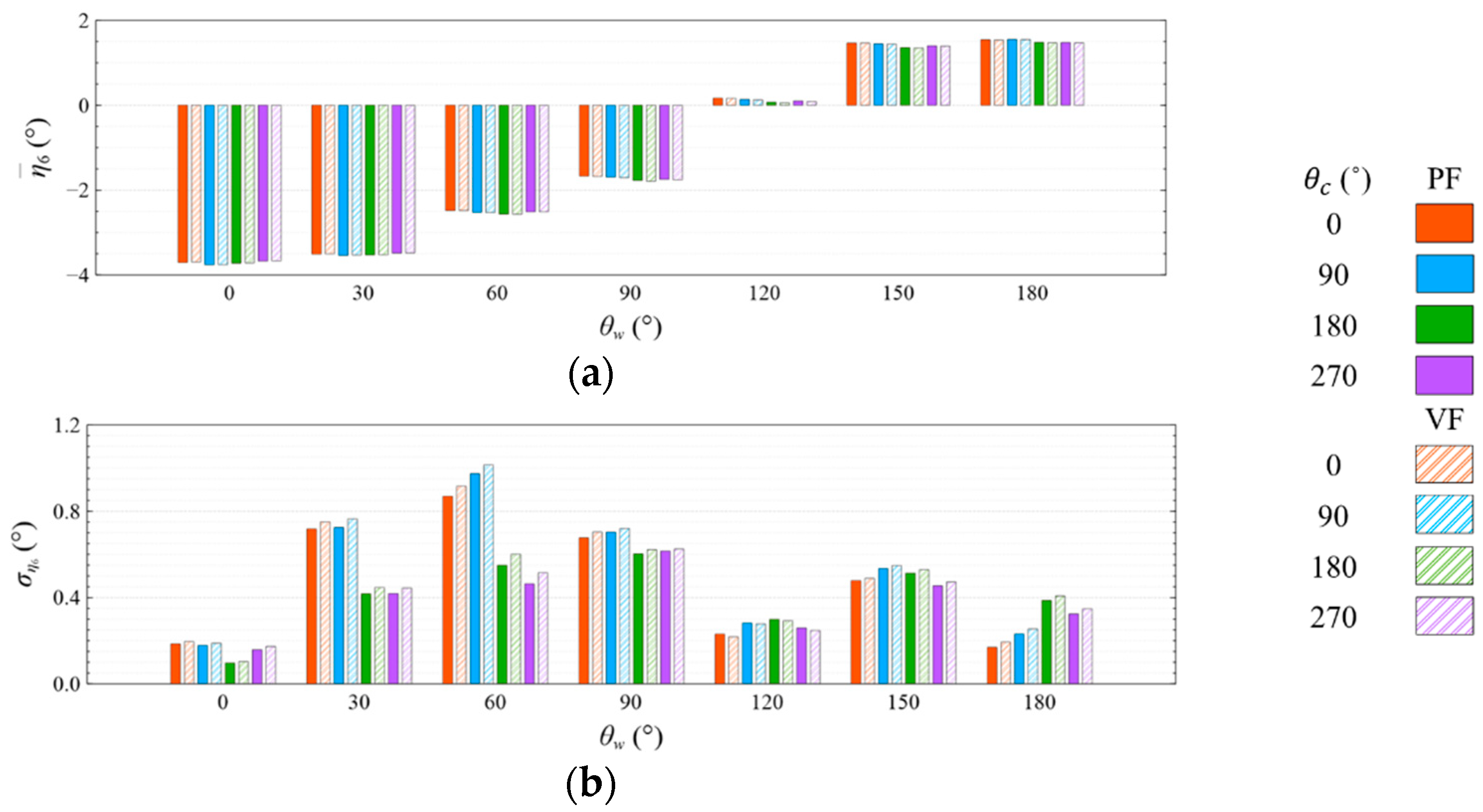
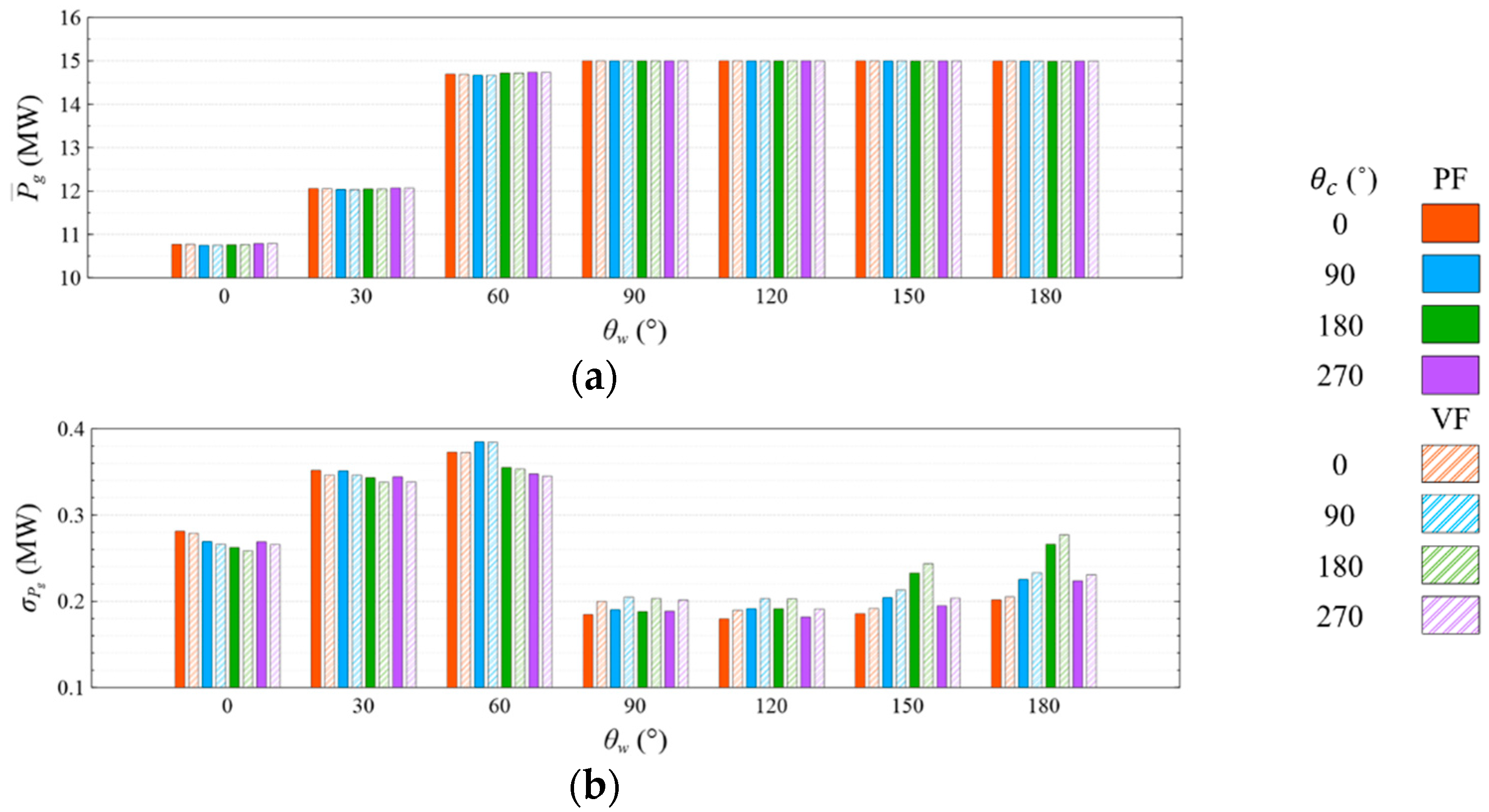
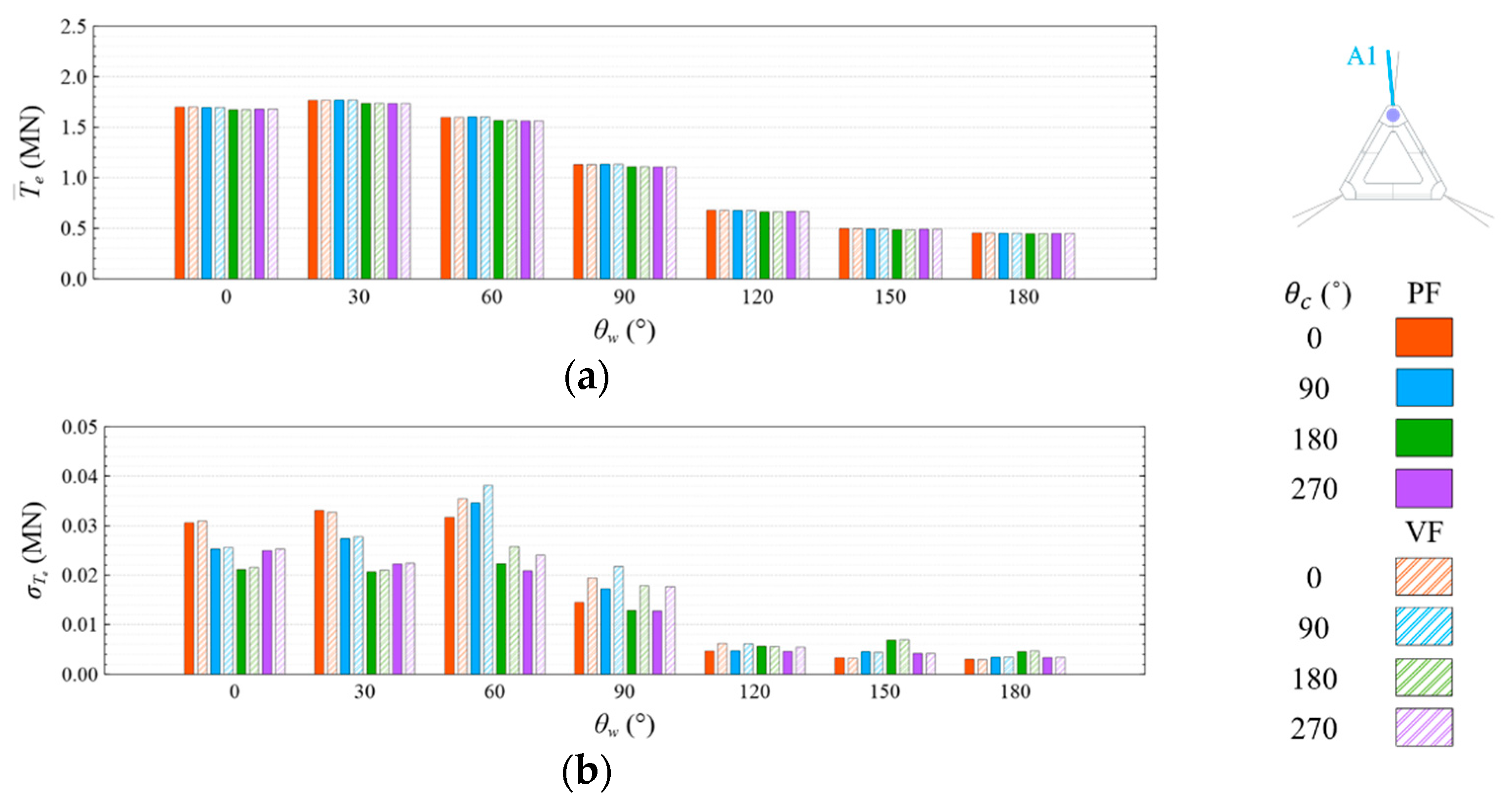
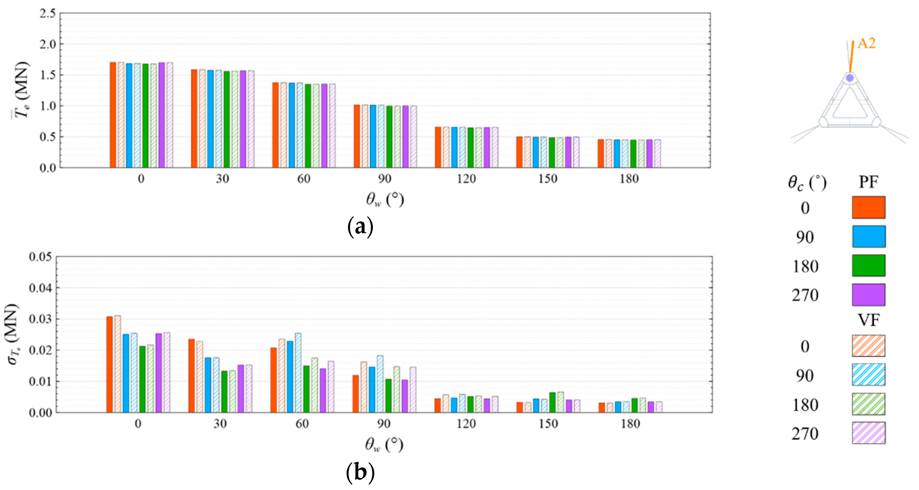
- The means and standard deviations of the motion response, generator power, and mooring line tension are obviously sensitive to the wind and wave directions, but they were insensitive to the viscous effect and current directions under both studied wave conditions. The influence of the viscous effect and current directions on the motion response and generator power mainly shows in the standard deviation rather than in the mean value;
- Under the CW condition, the generator power is relatively high and stable at to . Hence, to is the most favorable wind direction for the studied wind turbine system to operate under the CW condition in the Hsinchu offshore area, where the mean output power can reach 90% of the rated power. The occurrence of the most favorable power performance at to is clearly explained by the coupled platform motion with the motion-induced and wave-excited components because the center of gravity of the wind turbine system is off its geometrical center. The sums of the means and standard deviations of the mooring line tensions under the CW condition are all smaller than one-seventh of the break load of the mooring line;
- Under the HW condition, the generator power is relatively high and stable at to . Hence, to is the most favorable wind direction for the studied wind turbine system to operate under the HW condition in the Hsinchu offshore area, where the mean output power can reach 95% of the rated power. When compared with the CW results, it is obvious that the increase in the wind speed extends the favorable operation range in the incoming wind direction, as well as enhances the mean output power. The sums of the means and standard deviations of the mooring line tensions under the HW condition are all smaller than one-eighth of the break load of the mooring line;
- The most favorable wind direction range under the CW and HW conditions in this study is to , in which the corresponding motion responses all meet the design requirements, and the corresponding power output can reach 90% of the rated power. In the Taiwan Strait, the wind mostly comes from the northeast, with a probability of 40%, followed by the north–northeast, with a probability of 30%. Therefore, the angle between the leading mooring line of the system (i.e., Lines A1 and A2 in the study) and the most possible wind direction, which is the northeast, should be from 120° to 180° in order to deliver a relatively favorable performance.
Author Contributions
Funding
Institutional Review Board Statement
Informed Consent Statement
Data Availability Statement
Conflicts of Interest
Appendix A
Appendix A.1. Governing Equations


| Parameter | Value |
|---|---|
| ) | |
| 0.31 | |

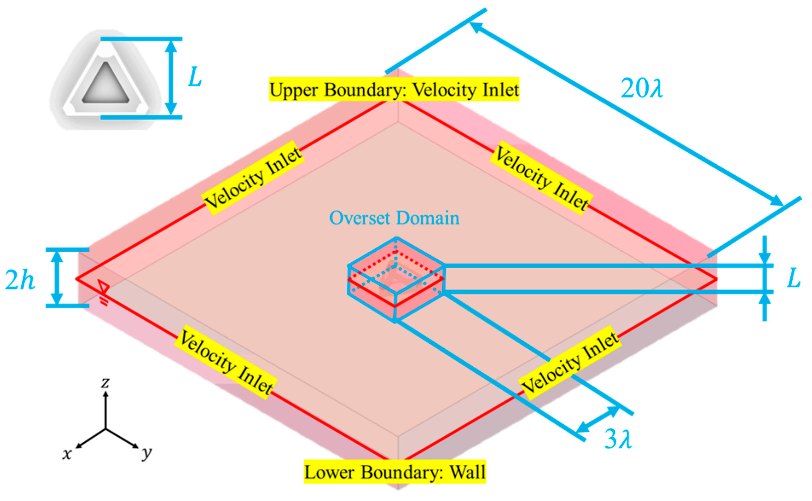
Appendix A.2. Setup of Modeling

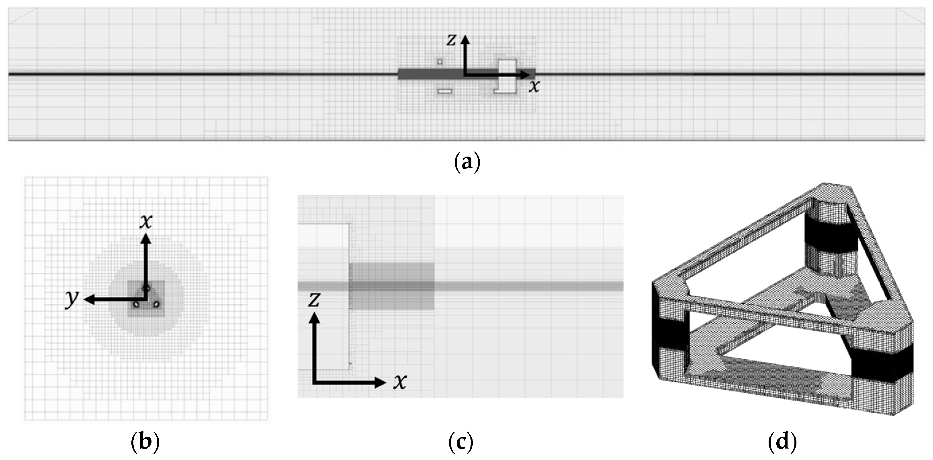
Appendix A.3. Setup of Mesh
| (a) | |||
|---|---|---|---|
| Properties (Unit) | CW Condition | HW Condition | |
| Platform Surface Mesh Faces | Surge, Sway, Yaw | 2.799 × 10⁵ | 2.793 × 10⁵ |
| Heave, Roll, Pitch | 6.459 × 10⁵ | 5.937 × 10⁵ | |
| Total Cell Numbers | Surge, Sway, Yaw | 3.413 × 10⁶ | 4.230 × 10⁶ |
| Heave, Roll, Pitch | 7.559 × 10⁶ | 8.096 × 10⁶ | |
| Platform Surface Mesh Size (m) | 0.625 | ||
| Platform Mesh Cell Size (m) | 6.25 | ||
| Maximum Background Mesh Cell Size (m) | 50 | ||
| (b) | |||
| Outer Boundary Shape | Outer Boundary of Refinement Region on-Plane from Origin | Cell Size Scale | |
| Cylinder | 1 | ||
| 1/2 | |||
| 1/4 | |||
| 1/8 | |||
| (c) | |||
| Properties (Unit) | CW Condition | HW Condition | |
| Region Thickness of Platform Mesh Refinement (m) | Surge, Sway, Yaw | 4 | 4 |
| Heave, Roll, Pitch | 11 | 10 | |
| Region Thickness of Background Mesh Refinement (m) | 2 | 2 | |
| Outer Boundary of Inner Refinement Region on -Plane | Circle with Radius of at Origin | ||
| Cell Size in -Direction (m) | Inner Region | 0.05 0.025 | |
| Outer Region | |||

References
- Global Wind Energy Council. Global Wind Report 2022. 2022. Available online: https://gwec.net/global-wind-report-2022/ (accessed on 22 August 2022).
- Open Access News. 2022. Offshore Wind Energy in Taiwan. Available online: https://www.openaccessgovernment.org/taiwan-offshore-wind/129010/ (accessed on 22 August 2022).
- Wind Resource Assessment Handbook. NREL/TAT-5–15283-01; National Renewable Energy Laboratory: Golden, CO, USA, 2011.
- Wang, Y.K.; Chai, J.F.; Chang, Y.W.; Huang, T.Y.; Kuo, Y.S. Development of Seismic Demand for Chang-Bin Offshore Wind Farm in Taiwan Strait. Energies 2016, 9, 1036. [Google Scholar] [CrossRef]
- Chang, T.J.; Chen, C.L.; Tu, Y.L.; Yeh, H.T.; Wu, Y.T. Evaluation of the Climate Change Impact on Wind Resources in Taiwan Strait. Energy Convers. Manag. 2015, 95, 435–445. [Google Scholar] [CrossRef]
- Uzunoglu, E.; Soares, C.G. Hydrodynamic design of a free-float capable tension leg platform for a 10 MW wind turbine. Ocean. Eng. 2020, 197, 106888. [Google Scholar] [CrossRef]
- Lee, Y.J.; Ho, C.Y.; Huang, Z.Z.; Wang, Y.C. Improvements on the Output of a Spar-Type Floating Wind Turbine Influenced by Wave-Induced Oscillation. J. Taiwan Soc. Nav. Archit. Mar. Eng. 2015, 34, 55–62. [Google Scholar]
- Huang, Z.Z. Dynamic Response of Floating Offshore Wind Turbine. Ph.D. Thesis, Department of Engineering Science and Ocean Engineering, National Taiwan University, Taipei, Taiwan, 2013. [Google Scholar]
- Wang, Y.C. Motion Characteristics and Power Evaluation on Floating Offshore Wind Turbine. Ph.D. Thesis, Department of Engineeri7ng Science and Ocean Engineering, National Taiwan University, Taipei, Taiwan, 2011. [Google Scholar]
- Chen, C.Y. Comparative Study on Semi-Submersible Floating Platforms for Offshore Wind in Taiwan Strait. Master’s Thesis, Department of Engineering Science and Ocean Engineering, National Taiwan University, Taipei, Taiwan, 2020. [Google Scholar]
- Hong, J.J. Performance Prediction of a Disk-Type Semi-Submersible Floating Platform in Taiwan Strait. Ph.D. Thesis, Department of Engineering Science and Ocean Engineering, National Taiwan University,, Taipei, Taiwan, 2022. [Google Scholar]
- Li, B.; Liu, K.; Yan, G.; Ou, J. Hydrodynamic Comparison of a Semi-Submersible, TLP, and Spar: Numerical Study in the South China Sea Environment. J. Mar. Sci. Appl. 2011, 10, 306–314. [Google Scholar] [CrossRef]
- De Guzman, S.; Maron, D.; Bueno, P.; Taboada, M. A Reduced Draft Spar Concept for Large Offshore Wind Turbines. In Proceedings of the 37th International Conference on Ocean, Offshore and Arctic Engineering, Madrid, Spain, 17–22 June 2018; American Society of Mechanical Engineers: New York, NY, USA, 2018. [Google Scholar]
- Quest Floating Wind Energy. 2022. Available online: https://questfwe.com (accessed on 22 August 2022).
- Jonkman, J.; Butterfield, S.; Musial, W.; Scott, G. Definition of a 5-MW Reference Wind Turbine for Offshore System Development. NREL/TP-500–38060; National Renewable Energy Laboratory: Golden, CO, USA, 2009. [Google Scholar]
- Bak, C.; Zahle, F.; Bitsche, R.; Kim, T.; Yde, A.; Henriksen, L.C.; Hansen, M.H.; Blasques, J.P.A.A.; Gaunaa, M.; Natarajan, A. The DTU 10-MW Reference Wind Turbine. In Proceedings of the Danish Wind Power Research, Fredericia, Denmark, 27−28 May 2013. [Google Scholar]
- Liu, J.; Manuel, L. Alternative Mooring Systems for a Very Large Offshore Wind Turbine Supported by a Semisubmersible Floating Platform. J. Sol. Energy Eng. 2018, 140, 051003. [Google Scholar] [CrossRef]
- Gaertner, E.; Rinker, J.; Sethuraman, L.; Zahle, F.; Anderson, B.; Barter, G.; Abbas, N.; Meng, F.; Bortolotti, P.; Skrzypinski, W.; et al. Definition of the IEA Wind 15-Megawatt Offshore Reference Wind Turbine; NREL/TP-5000–75698; National Renewable Energy Laboratory: Golden, CO, USA, 2020. [Google Scholar]
- Udoh, I.E.; Zou, J. Driving Down Cost: A Case Study of Floating Substructure for A 10MW Wind Turbine. In Offshore Technology Conference; OnePetro: Richardson, TX, USA, 2019. [Google Scholar]
- Zhang, Y.; Kim, B. A Fully Coupled Computational Fluid Dynamics Method for Analysis of Semi-Submersible Floating Offshore Wind Turbines Under Wind-Wave Excitation Conditions Based on OC5 Data. Appl. Sci. 2018, 8, 2314. [Google Scholar] [CrossRef]
- Tran, T.T.; Kim, D.H. Fully coupled aero-hydrodynamic analysis of a semi-submersible FOWT using a dynamic fluid body interaction approach. Renew. Energy 2016, 92, 244–261. [Google Scholar] [CrossRef]
- Robertson, A.; Jonkman, J.; Vorpahl, F.; Popko, W.; Qvist, J.; Froyd, L.; Chen, X.; Azcona, J.; Uzungoglu, E.; Guedes Soares, C. Offshore Code Comparison Collaboration, Continuation within IEA Wind Task 30: Phase II Results Regarding a Floating Semisubmersible wind System; National Renewable Energy Lab.: Golden, CO, USA, 2014. [Google Scholar]
- Luquet, R.; Ducrozet, G.; Gentaz, L.; Ferrant, P.; Alessandrini, B. Applications of the SWENSE method to seakeeping simulations in irregular waves. In Proceedings of the 9th International Conference on Numerical Ship Hydrodynamics, Ann Arbor, MI, USA, 5–8 August 2007. [Google Scholar]
- Sethuraman, L.; Venugopal, V. Hydrodynamic response of a stepped-spar floating wind turbine: Numerical modelling and tank testing. Renew. Energy 2013, 52, 160–174. [Google Scholar] [CrossRef]
- Antonutti, R.; Peyrard, C.; Johanning, L.; Incecik, A.; Ingram, D. An investigation of the effects of wind-induced inclination on floating wind turbine dynamics: Heave plate excursion. Ocean. Eng. 2014, 91, 208–217. [Google Scholar] [CrossRef]
- Nematbakhsh, A.; Olinger, D.J.; Tryggvason, G. Nonlinear simulation of a spar buoy floating wind turbine under extreme ocean conditions. J. Renew. Sustain. Energy 2014, 6, 033121. [Google Scholar] [CrossRef]
- Liu, Y.; Peng, Y.; Wan, D. Numerical Investigation on Interaction between a Semi-Submersible Platform and its Mooring System. In International Conference on Offshore Mechanics and Arctic Engineering; American Society of Mechanical Engineers: New York, NY, USA, 2015; p. 56550. [Google Scholar]
- Karimirad, M.; Michailides, C. V-shaped semisubmersible offshore wind turbine: An alternative concept for offshore wind technology. Renew. Energy 2015, 83, 126–143. [Google Scholar] [CrossRef]
- Zheng, X.Y.; Lei, Y. Stochastic response analysis for a floating offshore wind turbine integrated with a steel fish farming cage. Appl. Sci. 2018, 8, 1229. [Google Scholar] [CrossRef]
- Ishihara, T.; Zhang, S. Prediction of dynamic response of semi-submersible floating offshore wind turbine using augmented Morison’s equation with frequency dependent hydrodynamic coefficients. Renew. Energy 2019, 131, 1186–1207. [Google Scholar] [CrossRef]
- Lerch, M.; De-Prada-Gil, M.; Molins, C. The influence of different wind and wave conditions on the energy yield and downtime of a spar-buoy floating wind turbine. Renew. Energy 2019, 136, 1–14. [Google Scholar] [CrossRef]
- Zhang, P.; Yang, S.; Li, Y.; Gu, J.; Hu, Z.; Zhang, R.; Tang, Y. Dynamic response of articulated offshore wind turbines under different water depths. Energies 2020, 13, 2784. [Google Scholar] [CrossRef]
- Ferrandis, J.D.Á.; Bonfiglio, L.; Rodríguez, R.Z.; Chryssostomidis, C.; Faltinsen, O.M.; Triantafyllou, M. Influence of viscosity and non-linearities in predicting motions of a wind energy offshore platform in regular waves. J. Offshore Mech. Arct. Eng. 2020, 142, 062003. [Google Scholar] [CrossRef]
- Hsu, I.J.; Ivanov, G.; Ma, K.T.; Huang, Z.Z.; Wu, H.T.; Huang, Y.T.; Chou, M. Optimization of Semi-Submersible Hull Design for Floating Offshore Wind Turbines. In Proceedings of the ASME 2022 41st International Conference on Ocean, Offshore and Arctic Engineering, Hamburg, Germany, 5–10 June 2022. [Google Scholar]
- Huang, W.H. Influence of Water Depth Variation on the Mooring Line Design for FOWT in Shallow Waters. Master’s Thesis, Department of Hydraulic and Ocean Engineering, National Cheng Kung University, Tainan, Taiwan, 2021. [Google Scholar]
- DNV GL. DNVGL-RP-0286 Coupled Analysis of Floating Wind Turbines; DNV GL: Oslo, Norway, 2019. [Google Scholar]
- Ikhennicheu, M.; Lynch, M.; Doole, S.; Borisade, F.; Matha, D.; Dominguez, J.L.; Vicente, R.D.; Habekost, T.; Ramirez, L.; Potestio, S.; et al. D2.1 Review of the State of the Art of Mooring and Anchoring Designs, Technical Challenges and Identification of Relevant DLCs. Technical Report. CoreWind Project. 2020. Available online: https://corewind.eu/wp-content/uploads/files/publications/COREWIND-D2.1-Review-of-the-state-of-the-art-of-mooring-and-anchoring-designs.pdf (accessed on 22 August 2022). Technical Report. CoreWind Project.
- Gaertner, E.; Rinker, J.; Sethuraman, L.; Zahle, F.; Anderson, B.; Barter, G.; Abbas, N.; Meng, F.; Bortolotti, P.; Skrzypinski, W.; et al. 15MW Reference Wind Turbine Repository Developed in Conjunction with IEA Wind. 2022. Available online: https://github.com/IEAWindTask37/IEA-15–240-RWT/ (accessed on 22 August 2022).
- Chuang, T.C.; Yang, W.H.; Yang, R.Y. Experimental and Numerical Study of a Barge-Type FOWT Platform under Wind and Wave Load. Ocean. Eng. 2021, 230, 109015. [Google Scholar] [CrossRef]
- Jonkman, J.; Jason, M.L.; Marchall, B., Jr. FAST User’s Guide; National Renewable Energy Lab: Golden, CO, USA, 2005. [Google Scholar]
- Wehausen, J.V.; Laitone, E.V. Surface Waves in Fluid Dynamics III. In Handbuch der Physik; Springer Verlag: Berlin, Germany, 1960; Volume 9, pp. 446–778. [Google Scholar]
- Orcina. OrcaFlex Documentation Version 11.2d; Orcina: Ulverston, UK, 2022. [Google Scholar]
- Siemens. Simcenter STAR-CCM+ User Guide Version 2020.1; Siemens: Munich, Germany, 2020. [Google Scholar]
- Hirt, C.W.; Nichols, B.D. Volume of Fluid Method for the Dynamics of Free Surface. J. Comput. Phys. 1981, 39, 201–225. [Google Scholar] [CrossRef]


| Properties (Unit) | Value | |
|---|---|---|
| Draft (m) | 20 | |
| Total System Displacement (kton) | 23.683 | |
| Total System CG (m) | (4.117, 0, −2.29) | |
| Principal Inertias about CG (kg∙m2) | 4.932 × 10¹⁰ | |
| 5.335 × 10¹⁰ | ||
| 2.834 × 10¹⁰ | ||
| −6.734 × 10⁵ | ||
| −9.954 × 10⁹ | ||
| −3.047 × 10⁶ | ||
| Properties (Unit) | Value |
|---|---|
| Number of Mooring Lines | 3 × 2 |
| Angle between Adjacent Lines (°) | 10/119.8 |
| Depth to Anchors below SWL (m) | 70 |
| Depth to Fairleads below SWL (m) | 18 |
| Radius Measured from Centroid of Platform to Anchors (m) | 484.3 |
| Radius Measured from Centroid of Platform to Fairleads (m) | 47.1 |
| Unstretched Mooring Line Length (m) | 448 |
| Mooring Line Diameter (m) | 0.229 |
| Mooring Nominal Diameter (m) | 0.127 |
| Mooring Line Mass Density (kg/m) | 321 |
| Mooring Line Break Load (MN) | 14.96 |
| Mooring Line Axial Stiffness (GN) | 1.377 |
| Properties (Unit) | Value |
|---|---|
| Rated Power (MW) | 15 |
| Blade Length (m) | 120 |
| Hub Height (m) | 150 |
| Hub/Rotor Diameters (m) | 7.94/240 |
| Tower Base Diameter (m) | 10 |
| Hub Overhang (m) | 11.35 |
| Cut-in/Rated/Cut-out Wind Speeds (m/s) | 3/10.59/25 |
| Cut-in/Rated Rotor Speeds (RPM) | 5/7.56 |
| Shaft Tilt/Precone Angles (°) | 6/4 |
| Rotor Nacelle Assembly Mass (ton) | 1016.6 |
| Tower Mass (ton) | 860 |
| 3.5 | 4.5 | 5.5 | 6.5 | 7.5 | Sum | |
|---|---|---|---|---|---|---|
| 0.5 | 14.79% | 41.96% | 5.49% | 0.44% | 0.02% | 62.7% |
| 1.5 | 0.31% | 12.23% | 18.31% | 0.70% | - | 31.55% |
| 2.5 | - | 0.02% | 4.35% | 0.90% | 0.04% | 31.55% |
| 3.5 | - | - | - | 0.35% | 0.04% | 5.32% |
| 4.5 | - | - | - | 0.04% | 0.02% | 0.07% |
| Sum | 15.10% | 54.21% | 28.15% | 2.43% | 0.11% | 100% |
| Properties (Unit) | CW Condition | HW Condition |
|---|---|---|
| for JONSWAP Spectrum | 2.08 | 2.08 |
| (m) | 1.5 | 4.5 |
| (s) | 5.5 | 7.5 |
| (m/s) | 8.11 | 17.8 |
| (m/s) | 10.63 | 23.34 |
| (m/s) | 0.93 | 0.93 |
Disclaimer/Publisher’s Note: The statements, opinions and data contained in all publications are solely those of the individual author(s) and contributor(s) and not of MDPI and/or the editor(s). MDPI and/or the editor(s) disclaim responsibility for any injury to people or property resulting from any ideas, methods, instructions or products referred to in the content. |
© 2023 by the authors. Licensee MDPI, Basel, Switzerland. This article is an open access article distributed under the terms and conditions of the Creative Commons Attribution (CC BY) license (https://creativecommons.org/licenses/by/4.0/).
Share and Cite
Tong, H.-Y.; Lin, T.-Y.; Chau, S.-W. Normal Operating Performance Study of 15 MW Floating Wind Turbine System Using Semisubmersible Taida Floating Platform in Hsinchu Offshore Area. J. Mar. Sci. Eng. 2023, 11, 457. https://doi.org/10.3390/jmse11020457
Tong H-Y, Lin T-Y, Chau S-W. Normal Operating Performance Study of 15 MW Floating Wind Turbine System Using Semisubmersible Taida Floating Platform in Hsinchu Offshore Area. Journal of Marine Science and Engineering. 2023; 11(2):457. https://doi.org/10.3390/jmse11020457
Chicago/Turabian StyleTong, Hoi-Yi, Tsung-Yueh Lin, and Shiu-Wu Chau. 2023. "Normal Operating Performance Study of 15 MW Floating Wind Turbine System Using Semisubmersible Taida Floating Platform in Hsinchu Offshore Area" Journal of Marine Science and Engineering 11, no. 2: 457. https://doi.org/10.3390/jmse11020457
APA StyleTong, H.-Y., Lin, T.-Y., & Chau, S.-W. (2023). Normal Operating Performance Study of 15 MW Floating Wind Turbine System Using Semisubmersible Taida Floating Platform in Hsinchu Offshore Area. Journal of Marine Science and Engineering, 11(2), 457. https://doi.org/10.3390/jmse11020457