Hydroelastic Response to the Effect of Current Loads on Floating Flexible Offshore Platform

Abstract

An analytical model of a current load’s interaction with a moored floating flexible structure based on the Timoshenko–Mindlin beam theory is developed under the assumption of small-amplitude wave theory and the structural response. Theoretical solutions on the displacement of the structure, reflection, and transmission coefficients are obtained by applying the matching technique along with the orthogonal model coupling relation. The results of the transmission coefficient and displacement amplitude are compared with the other calculations and experimental datasets available in the literature. The structural deflection and transmission coefficients are investigated via the hydroelastic response for wave–current loads along with design parameters. The comparison results showed that the present model result is supported by the numerical model’s results. This present analysis can provide further information for marine engineers to design floating flexible platforms in the marine environment.

1. Introduction

Offshore floating structures are subjected to varied environmental loading including wind, waves, and currents. In the offshore region, waves never exist without an associated current. The modelling of wave–current loads seems to be explicitly critical, with little work available in the literature. Thomas and Klopman [1] addressed a full description of the flow field that considers the interaction between the waves and the current is never undertaken in the design of either coastal or offshore structures.

A numerical simulation method for calculating the dynamic properties of a floating bridge under wave, current, and moving loads was addressed in [2]. Huang et al. [3] investigated the hydrodynamic properties of three-dimensional bodies of arbitrary geometry subjected to the action of waves and weak currents in a channel based on the higher-order boundary element method. Latheef et al. [4] studied the typical design problem of calculating the ultimate base shear and overturning moments for slender fixed structures with the inclusion of the interaction between the currents and the wave field. An experimental study of a submerged plate in the presence of a current used as a breakwater for coastal area protection was performed in [5]. Chen and Basu [6] also proposed a model considering the wave–current interactions in dynamic analyses of floating offshore wind turbines (FOWTs) and investigated the interaction effects on the FOWT responses. The Reynolds-averaged Navier–Stokes equations were adopted to simulate the hydrodynamic coefficients induced by waves and currents for a stationary submerged circular cylinder in a two- dimensional numerical wave-current tank [7].

A comparison between the numerical and experimental response for a generic floating pontoon bridge structure for wave- and current-induced responses was performed in [8]. Lu and Yeung [9] considered unsteady hydroelastic waves caused by the interaction between fixed concentrated-line loads and the underlying current and found that the flexural gravity wave motion depended on the ratio of the current speed to phase or group speeds. Qua et al. [10] simulated and analyzed the dynamic responses of a Spar-type FOWT under the scenarios with a freak wave superimposed with a uniform current. Hydrodynamic and aerodynamic forces are calculated using the medium/small-scaled flow field nesting technology, which is brought into the structural dynamic equation for two-way iterative decoupling solving. Finally, hydroelastic responses of the floating bodies under typhoon–wave–current coupling effect and influencing mechanism are analyzed by a case study in [11].

The effects of underlying uniform current on the nonlinear hydroelastic waves generated due to an infinite floating plate are studied analytically in [12]. Bhattacharjee and Sahoo [13] used the dispersion relation to analyze detailed characteristics of the flexural gravity waves due to a floating elastic plate in the presence of a following current or an opposing current. Bispo et al. [14] studied a numerical and analytical model associated with wave interactions with a moored, articulated, very large floating structure composed of a set of hinged plates. A review of different models of very large floating structures (VLFS) comparing their advantages and disadvantages according to the depth in which their work was performed [15].

Floating structures have a considerable thickness, which generates rotary inertia and shear deformation [16]. Mohapatra and Guedes Soares [17] developed a three-dimensional general mathematical hydroelastic model dealing with the problem of wave interaction with a floating and submerged flexible structure based on small-amplitude wave theory and the linear structural response. Mohapatra and Guedes Soares [18] studied an analytical method associated with surface gravity wave interaction with a horizontal flexible floating and a submerged porous plate. A boundary integral equation method (BIEM) model for the problem of surface wave interaction with a moored, finite, floating flexible plate was performed in [19]. Mohapatra and Guedes Soares [20] also developed a hydroelastic model for the problem of linear wave interaction with a submerged horizontal flexible porous structure in finite water depth in three dimensions.

A 3D hydroelastic model subjected to linear wave interactions with horizontal flexible floating and submerged porous structures was developed based on Green’s function approach in water of finite and infinite depths [21]. Papathanasiou and Belibassakis [22] studied three approaches for the interaction of water waves with large floating elastic structures. The first model is based on the Euler–Bernoulli beam theory, the second is based on the Rayleigh beam equation, and the third approach utilizes the Timoshenko approximation. An analytical and numerical study of the hydroelastic behavior of the plate considering the diffraction of incident surface water waves by a very large floating structure of finite thickness and draft was performed [23]. Zilman and Miloh [24] considered a circular buoyant elastic plate of homogeneous stiffness floating in shallow water while the edge of the plate was free of shear forces and bending moments and the plate deflection was excited by a monochromatic ambient surface wave.

A literature review of the research on the hydroelastic analysis of pontoon-type very large floating structures (VLFS) and a brief introduction to VLFS was provided with the basic assumptions, equations, and boundary conditions for hydroelastic analysis of VLFS and the commonly used approaches for solving the problem in [25]. The effect of the oblique wave angle on the performance of anti-motion and hydroelastic behavior of VLFS was investigated numerically in the context of the direct time domain modal expansion theory [26]. Yoon et al. [27] addressed the maximum bending moment and deflection in plate structures and proposed a numerical procedure to analyze floating plate structures with multiple hinge connections in regular waves. The numerical method was applied to the hydrodynamic analysis of a two-dimensional very large floating platform and a plane incident wave for three different cases: Infinite, finite, and shallow water depths using BEM and the direct method [28].

Karperaki and Belibassakis [29] developed a two-dimensional frequency domain numerical method for VLFS hydroelasticity of inhomogeneous, elastic plates of varying thicknesses and negligible draft. A numerical approach employing a combination of the boundary element method and moving element method, which is named the BEM–MEM, was proposed by [30] to analyze the hydroelastic responses of floating composite plates subjected to moving loads. A numerical study on the motion and elastic response of a floating structure to the hydrodynamic loads using FEM was performed [31]. A review of fixed and floating offshore structures with sustainable design and management approaches was conducted [32]. Shumin et al. [33] investigated the dynamic properties of the wave and structure to determine the similitude parameters using a frequency response function approach.

A numerical study on the effects of connector and module stiffness on the hydroelastic response of a structure composed of flexible, interconnected modules was performed in [34]. A beam model and a 3D solid model of the support structure were developed to assess if the floating support platform structural elasticity has a substantial impact on the dynamic response of the platform, and the inertial forces, hydrodynamic added mass forces, hydrostatic, and mooring restoring forces were considered in the hydroelastic analysis by [35]. Kang and Kim [36] developed a numerical tool for a barge-type floating elastic body with various bending stiffnesses in the frequency domain.

The deformation of a moored floating flexible bar for different design parameters is based on the Timoshenko–Mindlin beam theory in two dimensions using an analytical approach studied in [37]. Some of the prominent works on the hydroelastic analysis of floating structures based on Mindlin’s thick plate theory can be found in [38,39]. The implementation of 3D experiments and assessment of the structural response of a floating breakwater along with its wave attenuation effectiveness under the action of perpendicular and oblique regular and irregular waves were investigated in [40]. An experimental investigation was carried out to measure combined wave and current loads on horizontally submerged square and rectangular cylinders [41]. A comparison of experimental data and a numerical study of the dynamic response of a floating bridge under the combined action of waves and currents was addressed in [42].

From the above studies, it is confirmed that, to date, there has been no mathematical model associated with wave–current interaction with floating flexible structures based on Timoshenko–Mindlin plate theory under the analytical approach and its analysis in the literature.

Therefore, here, a mathematical model of a floating horizontal flexible structure connected via mooring lines of finite dimensions in the presence of current speed based on the Timoshenko–Mindlin beam theory is developed to analyze the effect of current speed and mooring lines on the hydroelastic response of a floating flexible structure in the practical problem for engineering interest.

The new contributions of the present hydroelastic model compared with [37] are the mathematical formulation and analytical solutions in the presence of current speed, the comparisons of the present analysis with the existing published numerical results, other calculation results, and experimental datasets, and the free with the moored floating structure for different current speeds. Furthermore, the effect of current speed along with different design parameters on the moored floating flexible structure for the hydroelastic response is investigated by analyzing structural displacements and transmission coefficients in different cases.

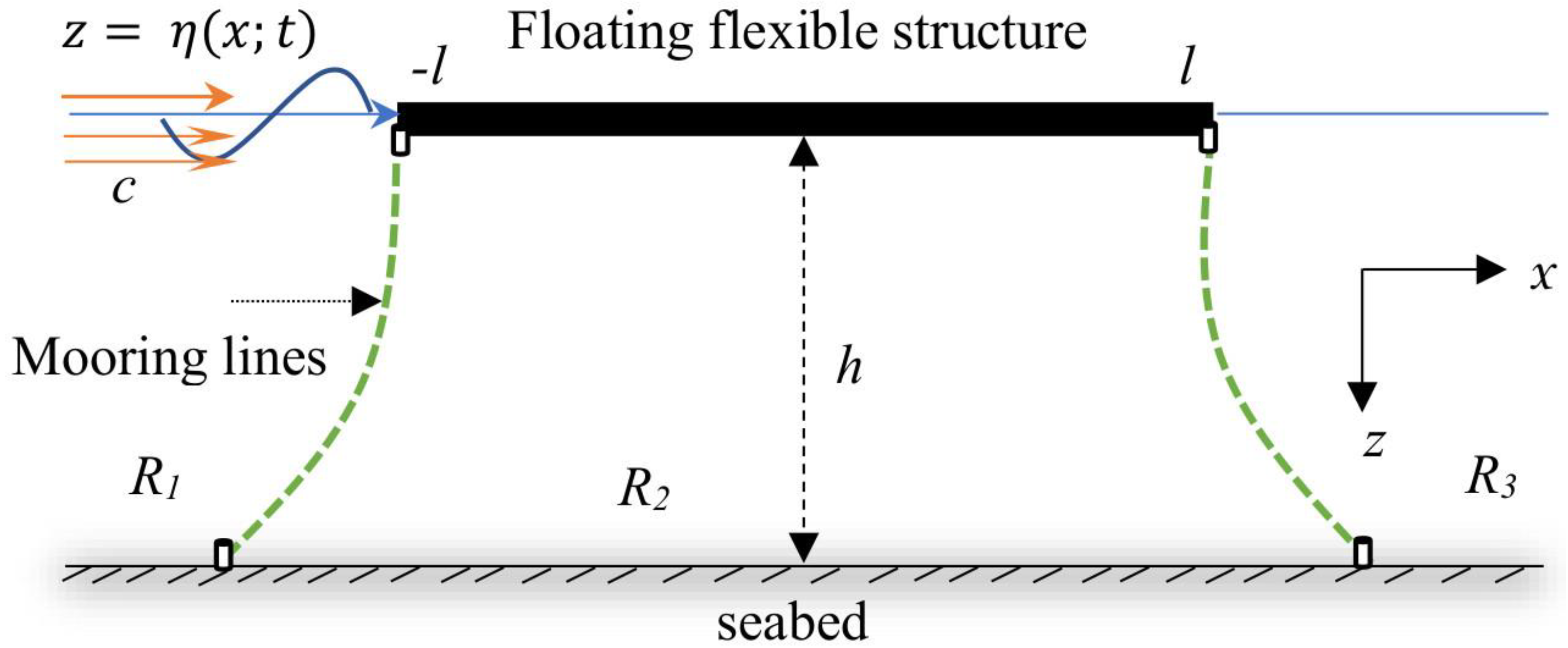
2. Model Definition

The formulation of the hydroelastic model is based on the assumption of the small-amplitude linearized water wave theory and structural response in two dimensions in water of a finite depth. The floating beam is modelled as the Timoshenko–Mindlin beam theory of finite length $2l$ with thickness $d$ and occupies the region $-l<x<l$ on the mean free surface $z=0$ over an impermeable sea bed $z=h$. It is considered that the floating beam is connected via mooring lines with stiffness $k_j$ for j = 1,2 at the edges of the structure at $x=l,-l$ (see Figure 1). Furthermore, it is also assumed that there is a uniform current flowing with constant speed $c=c·\cos \theta$ along the direction of wave propagation in the positive direction of the x-axis with an angle of $\theta$ referred to as the following current.

Hence, the whole fluid domain is divided into three subregions designated as $x\in (-\infty ,-l),z\in (0,h) \mathrm{by} R_1$, $x\in (-l,l),z\in (0,h) \mathrm{by} R_2,$ and $x\in (l,\infty ),z\in (0,h) \mathrm{by} R_3$. It is assumed that the fluid is inviscid and incompressible, and the motion is irrotational. Therefore, therefore the total velocity potential ${\mathsf{\Psi }}_j(x,z;t)$ for $j=1,2,3$ associated with the current speed $c$ and the direction of wave propagation (along the positive direction of the x-axis) can be expressed (as in [43]) as:

$${\mathsf{\Psi }}_j(x,z;t)=cx+{\mathsf{\Phi }}_j(x,z;t) \mathrm{for} j=1,2,3,$$

(1)

where ${\mathsf{\Phi }}_j(x,z;t)=Re\left\{{\varphi }_j(x,z)e^{-i\omega t}\right\}$ with ${\varphi }_j(x,z)$ is the partial velocity potential and Re is the real part of the complex velocity potential. Furthermore, the displacement of the floating flexible beam is assumed to be of the form $\eta (x;t)=\mathrm{Re}\{\eta (x)e^{-i\omega t}\}$. Hence, the velocity potentials ${\mathsf{\Phi }}_j(x,z;t)$ satisfy the 2D Laplace equation as

$${\nabla }_{xz}^2{\mathsf{\Phi }}_j=0, \mathrm{in} \mathrm{the} \mathrm{fluid} \mathrm{domain}.$$

(2)

The linear form of the free surface boundary condition in $R_1$ and $R_3$ in the presence of the following current $c$ at $z=0$ is given by (as in [43])

$$g\frac{\partial {\mathsf{\Phi }}_j}{\partial z}={\left(\frac{\partial }{\partial t}+c\frac{\partial }{\partial x}\right)}^2{\mathsf{\Phi }}_j, j=1,3, x\in (-\infty ,-l)\cup (l,\infty ),$$

(3)

where $g$ is the gravitational constant. It may be mentioned that if we set the current speed to $c=0$ in Equation (3), then the reduced free-surface condition is the same as in [37] and [19] in the case of a floating elastic plate.

As the bottom is rigid, the bottom boundary condition yields

$$\frac{\partial {\mathsf{\Phi }}_j}{\partial z}=0 \mathrm{for} j=1,3 \mathrm{on} z=h.$$

(4)

The linearized kinematic boundary condition in the presence of the following current c on the beam-covered surface is given by

$$\frac{\partial \eta }{\partial t}+c\frac{\partial \eta }{\partial x}=\frac{\partial {\mathsf{\Phi }}_j}{\partial z} \mathrm{for} j=2, \mathrm{on} z=0.$$

(5)

The hydrodynamic pressure $P_H$ exerted on the floating beam at $z=0$ under the following current $c$ is given by

$$P_H(x,t)=-\rho \left(\frac{\partial }{\partial t}+c\frac{\partial }{\partial x}\right){\mathsf{\Phi }}_j+\rho g\eta .$$

(6)

Using Equations (5) and (6) in the governing equation of Timoshenko–Mindlin beam theory under the effect of rotary and shear deformation, the beam-covered boundary condition under the influence of the following current c is obtained as

$$\begin{array}{l}\{EI\frac{{\partial }^4}{\partial x^4}-\left(\frac{EI{\rho }_b}{\mu G}+\frac{{\rho }_b{d}^3}{12}\right)\frac{{\partial }^2}{\partial t^2}\frac{{\partial }^2}{\partial x^2}+\frac{{\rho }_b^2{d}^3}{12\mu G}\frac{{\partial }^4}{\partial t^4}+{\rho }_{b}d\frac{{\partial }^2}{\partial t^2}\}\left(\frac{\partial \eta }{\partial t}+c\frac{\partial \eta }{\partial x}\right)\\ =-\left(1-\frac{EI}{\mu Gd}\frac{{\partial }^2}{\partial x^2}+\frac{{\rho }_b{d}^2}{12\mu G}\frac{{\partial }^2}{\partial t^2}\right)\left\{\rho {\left(\frac{\partial }{\partial t}+c\frac{\partial }{\partial x}\right)}^2{\mathsf{\Phi }}_2-\rho g\left(\frac{\partial \eta }{\partial t}+c\frac{\partial \eta }{\partial x}\right)\right\}.\end{array}$$

(7)

The beam-covered boundary condition (7) in R₂ can be expressed in terms of ${\mathsf{\Phi }}_2$ (refers to the velocity potential in R₂) by using Equation (5) as

$$\begin{array}{c}\{EI\frac{{\partial }^4}{\partial x^4}-\left(\frac{EI{\rho }_b}{\mu G}+\frac{{\rho }_b{d}^3}{12}\right)\frac{{\partial }^2}{\partial t^2}\frac{{\partial }^2}{\partial x^2}+\frac{{\rho }_b^2{d}^3}{12\mu G}\frac{{\partial }^4}{\partial t^4}+{\rho }_{b}d\frac{{\partial }^2}{\partial t^2}\\ +\rho g\left(1-\frac{EI}{\mu Gd}\frac{{\partial }^2}{\partial x^2}+\frac{{\rho }_b{d}^2}{12\mu G}\frac{{\partial }^2}{\partial t^2}\right)\}\frac{\partial {\mathsf{\Phi }}_2}{\partial z}\\ =-\left(1-\frac{EI}{\mu Gd}\frac{{\partial }^2}{\partial x^2}+\frac{{\rho }_b{d}^2}{12\mu G}\frac{{\partial }^2}{\partial t^2}\right)\left\{\rho {\left(\frac{\partial }{\partial t}+c\frac{\partial }{\partial x}\right)}^2{\mathsf{\Phi }}_2\right\}, \end{array}$$

(8)

where $\chi =(\rho g-m_s{\omega }^2)$ with ${\rho }_b$, $\mu$, $G=E/2(1+\mu )$, $d$, $EI$, and ${\rho }_{b}d=m_s$ are the density, transverse deformation, shear modulus, thickness, rigidity, and mass of the beam, respectively.

As the floating flexible beam is connected with mooring lines to the bottom with stiffness $k_j, j=1,2$ and $x=\pm l$ yield

$$\frac{{\partial }^3{\varphi }_2(x,z)}{\partial z^3}=0, x=\pm l, z=0,$$

(9)

$$\frac{{\partial }^4{\varphi }_2(x,z)}{\partial z^3\partial x}-\left\{\frac{m_s{\omega }^2(I_r+S_d)}{EI}\right\}\frac{\partial {\varphi }_2(x,z)}{\partial x}=k_j\frac{\partial {\varphi }_2(x,z)}{\partial z}, x=\pm l, z=0.$$

(10)

where $I_r$ and $S_d$ are the rotary inertia and shear deformation of the floating flexible beam.

The continuity of pressure and velocity at the vertical interface $\mathrm{x}=l,-l$ on $0<z<h$ is given by

$${\varphi }_j={\varphi }_{j+1} \mathrm{at} x=-l \mathrm{for} j=1 \mathrm{and} x=l \mathrm{for} j=2,$$

(11)

$$\frac{\partial {\varphi }_j}{\partial x}=\frac{\partial {\varphi }_{j+1}}{\partial x} \mathrm{at} x=-l \mathrm{for} j=1 \mathrm{and} x=l \mathrm{for} j=2.$$

(12)

Finally, the far-field condition at infinity is assumed to take the form

$$\varphi (x,z)=\{\begin{array}{l}\left(I_0{e}^{i{\mu }_{0}x}+R_0{e}^{-i{\mu }_{0}x}\right)f_0(z) \mathrm{as} x\to -\infty ,\\ T_0{e}^{i{\mu }_{0}x}{f}_0(z) \mathrm{as} x\to \infty ,\end{array}$$

(13)

where $I_0$ = incident wave amplitude, and $R_0$ and $T_0$ are the amplitudes of the waves associated with the reflected and transmitted waves, respectively. Furthermore, $f_0(z)=\left\{\cosh {\mu }_0(h-z)/\cosh {\mu }_{0}h\right\}$ with ${\mu }_0$ satisfies the gravity wave dispersion relation ${(\omega -c{\mu }_n)}^2=g{\mu }_0\tanh {\mu }_{0}h$.

3. Method of Solution

The formulation of the hydroelastic model is based on the assumption of the small-amplitude linearized theory. Using the Fourier expansion formulae and the method of the separation of variables, the velocity potentials ${\varphi }_1, {\varphi }_2,$ and ${\varphi }_3$ satisfying Equation (2) and boundary conditions (3, 4, 8) are expanded as:

$${\varphi }_1(x,z)=\frac{-ig{I}_o}{2(\omega -c{\mu }_0)}{f}_0(z)e^{i{\mu }_0(x+l)}-\frac{ig}{2(\omega -c{\mu }_n)}{\displaystyle \sum _{n=0,1}^{\infty }{R}_n{f}_n(z)e^{-i{\mu }_n(x+l),}}$$

(14)

$${\varphi }_2(x,z)=\frac{-ig}{2(\omega -c{\lambda }_n)}\left\{{\displaystyle \sum _{n=0,I}^{II}(A_n{e}^{-i{\lambda }_{n}x}+B_n{e}^{i{\lambda }_{n}x})v_n(z)}+{\displaystyle \sum _{n=1}^{\infty }(A_n{e}^{{\lambda }_{n}x}+B_n{e}^{-{\lambda }_{n}x})v_n(z)}\right\},$$

(15)

$${\varphi }_3(x,z)=\frac{-ig}{2(\omega -c{\mu }_n)}{\displaystyle \sum _{n=0,1}^{\infty }{T}_n{e}^{i{\mu }_n(x-l)}{f}_n(z),}$$

(16)

where

$$f_n(z)=\frac{\cos {\mu }_n(h-z)}{\cos {\mu }_{n}h}, v_n(z)=\frac{\cosh {\lambda }_n(h-z)}{\cosh {\lambda }_{n}h.}$$

(17)

Furthermore, $f_0(z)$ and ${\mu }_0$ are the same as defined in Equation (13) with ${\mu }_n=i{\mu }_n$ satisfied with the following dispersion relations (as in [6,43])

$${(\omega -c{\mu }_n)}^2=\{\begin{array}{l}g{\mu }_0\tanh ({\mu }_{0}h) \mathrm{for} n=0,\\ -g{\mu }_n\tan ({\mu }_{n}h) \mathrm{for} n=1,2,\dots \end{array}$$

(18)

and $f_n(z)$ in $R_1$ and $R_3$ are orthogonally defined by:

$$\langle f_m, f_n\rangle =\{\begin{array}{l}0 \mathrm{for} m\pm n,\\ C_n=\{\begin{array}{l}\left(2{\mu }_{0}h+\sinh 2{\mu }_{0}h\right)/4{\mu }_0{\cosh }^2{\mu }_{0}h, n=0\\ (2{\mu }_{n}h+\sin 2{\mu }_{n}h)/4{\mu }_n{\cos }^2{\mu }_{n}h, n=1,2,\dots ,\end{array} \mathrm{for} m=n,\end{array}$$

(19)

and ${\lambda }_n$ satisfies the dispersion relation for $n=0$ and $n=1,2,\dots$ with ${\lambda }_n=i{\lambda }_n$ as:

$$(\alpha {\lambda }_n^4-\beta {\lambda }_n^2+\gamma ){\lambda }_n\tanh {\lambda }_{n}h-({\kappa }_1+{\kappa }_2{\lambda }_n^2){(\omega -c{\lambda }_n)}^2=0,$$

(20)

and $v_n(z)$ in $R_2$ is orthogonally defined by

$$v_{ORT}=\langle v_m, v_n\rangle =\{\begin{array}{l}0 \mathrm{for} m\pm n,\\ Q_n \mathrm{for} m=n,\end{array}$$

(21)

where

$$\begin{array}{l}{Q}_n=[\{2{\lambda }_{n}h+\sinh (2{\lambda }_{n}h)\}\mathsf{\Lambda }({\lambda }_n)\mathsf{\Upsilon }({\lambda }_n)+4{\lambda }_n^3\mathsf{\Upsilon }({\lambda }_n)(2{\lambda }_n^2\gamma -\beta ){\sinh }^2({\lambda }_{n}h)\\ +4{\kappa }_2{\lambda }_n\mathsf{\Lambda }({\lambda }_n){\cosh }^2({\lambda }_{n}h)]/\{4{\lambda }_n\mathsf{\Upsilon }({\lambda }_n)\mathsf{\Lambda }({\lambda }_n){\cosh }^2({\lambda }_{n}h)\}\end{array}$$

$$\begin{array}{l}\langle v_m, v_n\rangle ={\displaystyle \underset{0}{\overset{h}{\int }}{v}_m(z) v_n(z)dz}+\frac{\gamma }{\mathsf{\Lambda }({\lambda }_n)}{\{v_m^{‴}(z)v_n^{\prime }(z)+v_m^{\prime }(z)v_n^{‴}(z)\}|}_{z=0}\\ -\frac{\beta }{\mathsf{\Lambda }({\lambda }_n)}{v_m^{\prime }(z)v_n^{\prime }(z)|}_{z=0}+\frac{{\kappa }_2}{\mathsf{\Upsilon }({\lambda }_n)}{v_m(z)v_n(z)|}_{z=0}\end{array}$$

(22)

with $\alpha =EI$, $\beta =\{m_s{\omega }^2(I_r+S_d)-S_d\rho g\}$, $\gamma =\{-m_s{\omega }^2{I}_r{S}_d\chi /EI\}+\chi$, ${\kappa }_1=\rho S_d$, ${\kappa }_2=\rho \{1-(m_s{w}^2{I}_r{S}_d)/EI\}$, $\mathsf{\Upsilon }({\lambda }_n)=(\alpha {\lambda }_n^4-\beta {\lambda }_n^2+\gamma )$, and $\mathsf{\Lambda }({\lambda }_n)=({\kappa }_1+{\kappa }_2{\lambda }_n^2){(\omega -c{\lambda }_n)}^2$.

It is worth mentioning that if we set the constant current speed $c=0$ in Equation (18) and in Equation (20), the reduced dispersion relation will be the same as in the case without a current in [19] for water dispersion relation and in [37] for the beam-covered dispersion relation without a current, respectively.

The procedure for the determination of unknown coefficients $R_n,T_n,A_n,B_n$ associated with Equations (14)–(16) is presented in Appendix A.

Once the unknown constants R₀ and T₀ are determined, the full solution is obtained in terms of the potential functions with the reflection coefficient $C_r$ and transmission coefficient $C_t$ obtained by using the formulae $C_r=\left|R_0\right|$ and $C_t=\left|T_0\right|$, respectively.

Determination of Displacement and Shear Force

The vertical displacement of the floating flexible structure in the presence of the current speed $c$ can be obtained from the following condition:

$$\left(\frac{\partial }{\partial t}+c\frac{\partial }{\partial x}\right)\eta (x,t)=\frac{\partial {\mathsf{\Phi }}_2}{\partial z.}$$

(23)

The shear force acting on the horizontal flexible floating structure can be computed by the formula:

$$S_f=\left|\left[{\partial }_{xzzz}-[\{m_s{\omega }^2(I_r+S_d)\}/EI]{\varphi }_{2x}(x,z)\right]-k{\varphi }_{2z}(x,z)\right| \mathrm{at} x=\pm l, z=0$$

(24)

To understand the effect of the current speed along with different design parameters associated with the model developed, several numerical results on the displacements and transmission coefficients and the comparison with/without the current speed are analyzed.

4. Numerical Results and Discussion

In the numerical computations, all simulations are executed by considering the values as mentioned in

Table 1. Model properties.

Model Parameters	Ranges of Values	Units
Non-dimensional water depth (h/l)	0.5	[-]
Non-dimensional wavenumber (${\mu }_{0}h$)	0–14	[-]
Non-dimensional thickness ($d/l$)	0.03	[-]
Current speed ($c$)	0.02–1.3	[m/s]
Mooring stiffness ($k$)	0.25	[N/m]
Water density ($\rho$)	1025	[kgm−3]
Gravitational constant ($g$)	9.8	[m/s]
Elastic modulus ($E$)	10–50	[GPa]

, unless stated otherwise. MATLAB R2016b, 64-bit (win64) is used to perform calculations in a desktop machine with Intel^® core i7-4790 CPU with a 3.60 GHz processor and 8 GB of RAM, 3601 MHz, 4 Core(s), and 8 Logical Processor(s) based on the analytical solution. Each case took approximately 10–15 min to finish.

It may be noted that to avoid repetition, the convergence analysis of the displacements with increasing values of N is deferred here (see [37]). However, the number of terms in the series solution to present the numerical results are taken as $N\ge 43$ for the computational accuracy of the numerical simulations. In the context of the present numerical results, the new contribution is the presentation of the numerical analysis with the effect of the current speed and comparison between them in terms of with and without the current speed, a moored and freely floating structure with current speed, and finally, an individual analysis for different design parameters.

4.1. Comparison Results

In Figure 2, the comparison between the present results of the transmission coefficient $C_t$ and the numerical BIEM results (see [28]) versus the non-dimensional wavelength $\lambda /l$ with elastic modulus $E=62 \mathrm{GPa}$ and water depth $h=50 \mathrm{m}$ with current speed $c=0.02 \mathrm{m}/\mathrm{s}$ are presented. A high value of elastic modulus and a very small value of current speed are chosen for a similar trend between the results from the model [28] and the present.

The comparison indicates that the present model solution is supported by the numerical BIEM model simulation. However, the differences can be explained by the formulation under the assumption of Timoshenko–Mindlin beam theory of the present model with current speed c and thin plate theory in [28]. Furthermore, the effect of the elastic modulus in the present model leads to higher rigidity that results in lower transmission. Furthermore, in Figure 2, the transmission coefficient from the BIEM model is 1 m, while the present model is 0.97 m, which is 3% larger.

Figure 3 shows the comparison between the present results against other calculation results [44] and experimental datasets [45] available in the literature versus the positive direction of $l(\mathrm{m})$ for the elastic modulus $E= 14 \mathrm{GPa}$ and mooring stiffness $k={ 10}^{0.02} \mathrm{N}/\mathrm{m}$. A certain value of elastic modulus and a very small value of mooring stiffness, with the range of current speed mentioned in Table 1, are chosen for a similar trend between the results from the model [44] and experimental datasets [45] with the present results. It is observed that the present result of the displacement amplitude is supported by the other calculations and experimental datasets available in the literature.

However, in Figure 3, the discrepancies between the present results and models from [44,45] may be clarified by the values of the mooring stiffness of the present results and the free-floating structure in the model [44] with the values of the elastic modulus in MPa (unit). The effect of mooring stiffness in the case of the present model leads to lower displacement than that of the previous model [44]. Therefore, it is suspected that the model presented in [44] produces higher displacement that the present model cannot reproduce. In addition, in Figure 3, the displacement amplitude from the previous [44] model is approximately 0.24 m, while the present model is 0.18 m, which is 6% larger.

Figure 4 shows the comparison of displacement between cases without and with current versus structural length l(m) with $k={ 10}^9 \mathrm{N}/\mathrm{m}$. It is seen that displacement without the current speed becomes lower than that of displacements with the current speed. This is due to the current providing hydrodynamic forces, which results in a higher displacement with a certain value of mooring stiffness and elastic modulus of the structure.

Figure 5 compares the displacements of the moored (with $k={10}^9 \mathrm{N}/\mathrm{m}$) and freely floating structure versus the structural length l(m) for different current speeds as is mentioned in the legend. From Figure 4, for different values of current speed c, it can be easily seen that the displacements of the freely floating structure are higher than that of the moored one. This is the result of the mooring lines connected to the floating structure that lead the structure in place with lower deflection.

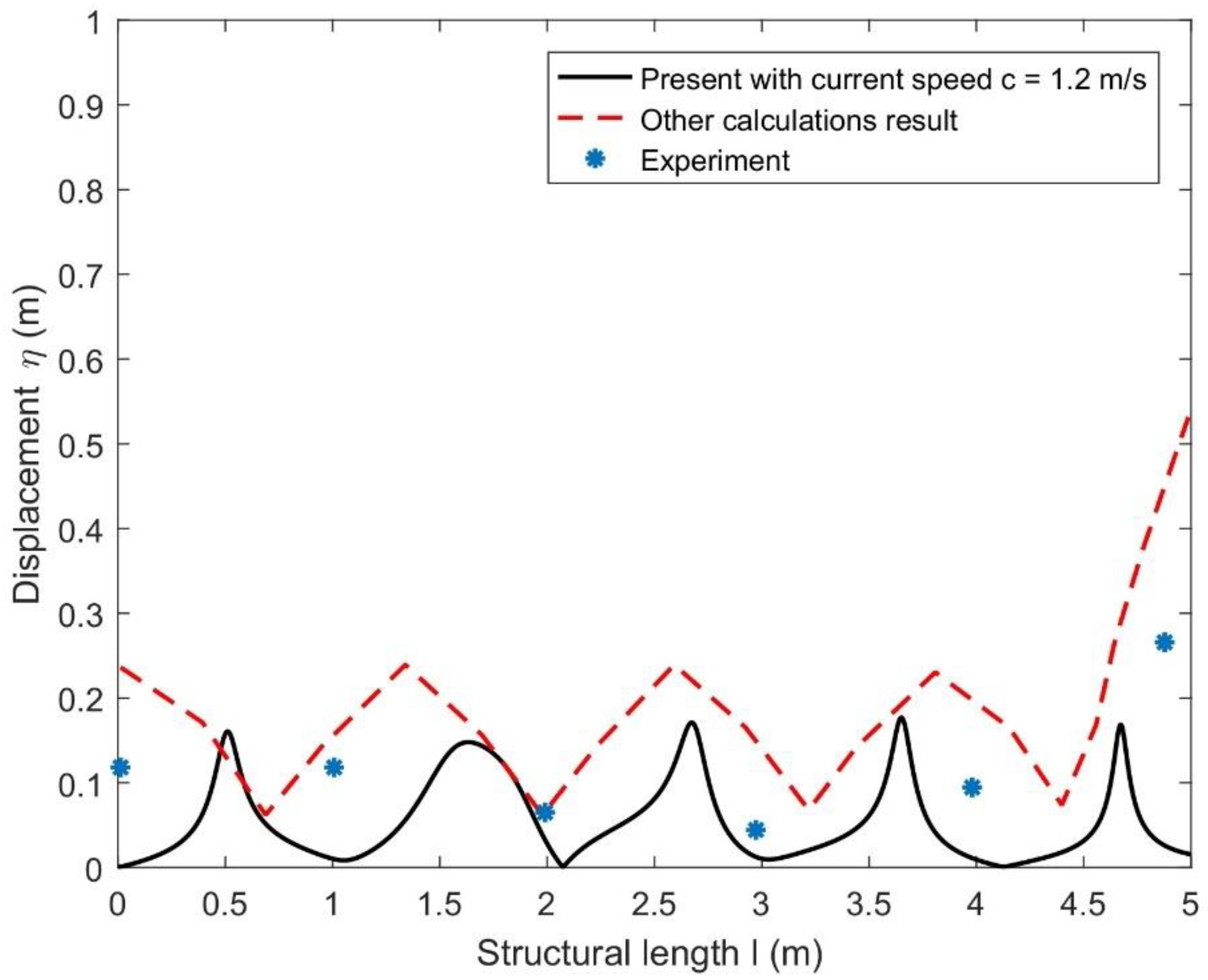
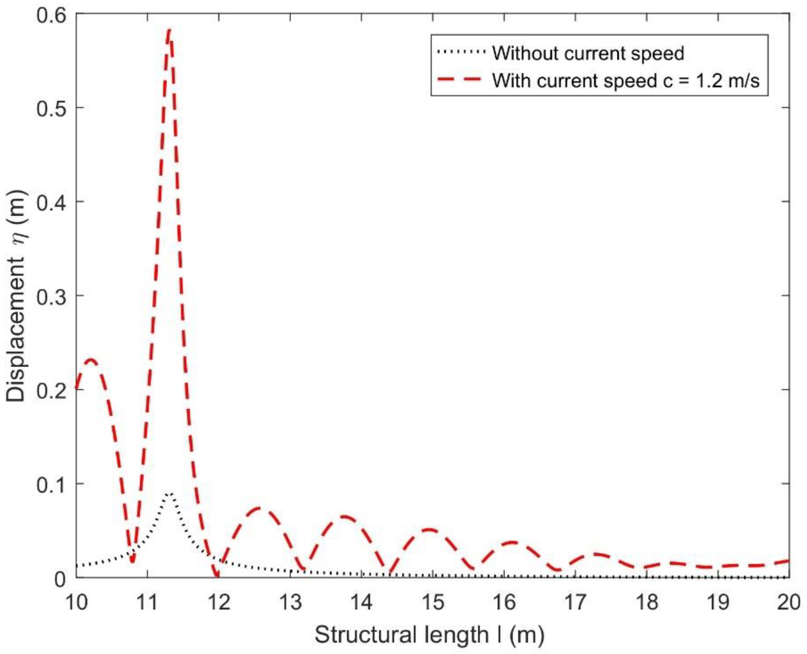
4.2. Hydroelastic Response Analysis via Displacements of Floating Structure

Figure 6 presents the displacements of floating flexible structures for different current speeds $c$ versus a non-dimensional structural length l(m) with the same parametric values as mentioned in Table 1. It is observed that the displacement of the flexible structure becomes higher as the current speed increases. A larger current provided larger hydrodynamic forces, which results in a higher displacement with a certain value of mooring stiffness and elastic modulus of the structure.

Figure 7 shows the structural displacements for different values of the elastic modulus $E$ versus the structural length l(m) with other parametric values being the same as mentioned in Table 1. With the increase in the elastic modulus, the displacement decreases, which indicates that increasing the elastic modulus can effectively prevent the deformation of the floating structure as the structural rigidity becomes higher.

Figure 8 simulates the effect of displacements for different mooring stiffness values $k$ versus structural length l(m) with the current speed $c=1.0 \mathrm{m}/\mathrm{s}$ and elastic modulus $E=15 \mathrm{GPa}$. It can be easily seen that by increasing the mooring stiffness, the deformation of the floating structure decreases, which suggests that higher stiffness prevents the deformation that leads to more stability in the structure.

In the next subsection, only the transmission coefficient $C_t$ is discussed in the presence of the current speed along with different physical parameters associated with the referred model because the reflection coefficient $C_r$ is of the opposite trend to that of $C_t$. Therefore, the numerical computation $C_r$ is deferred.

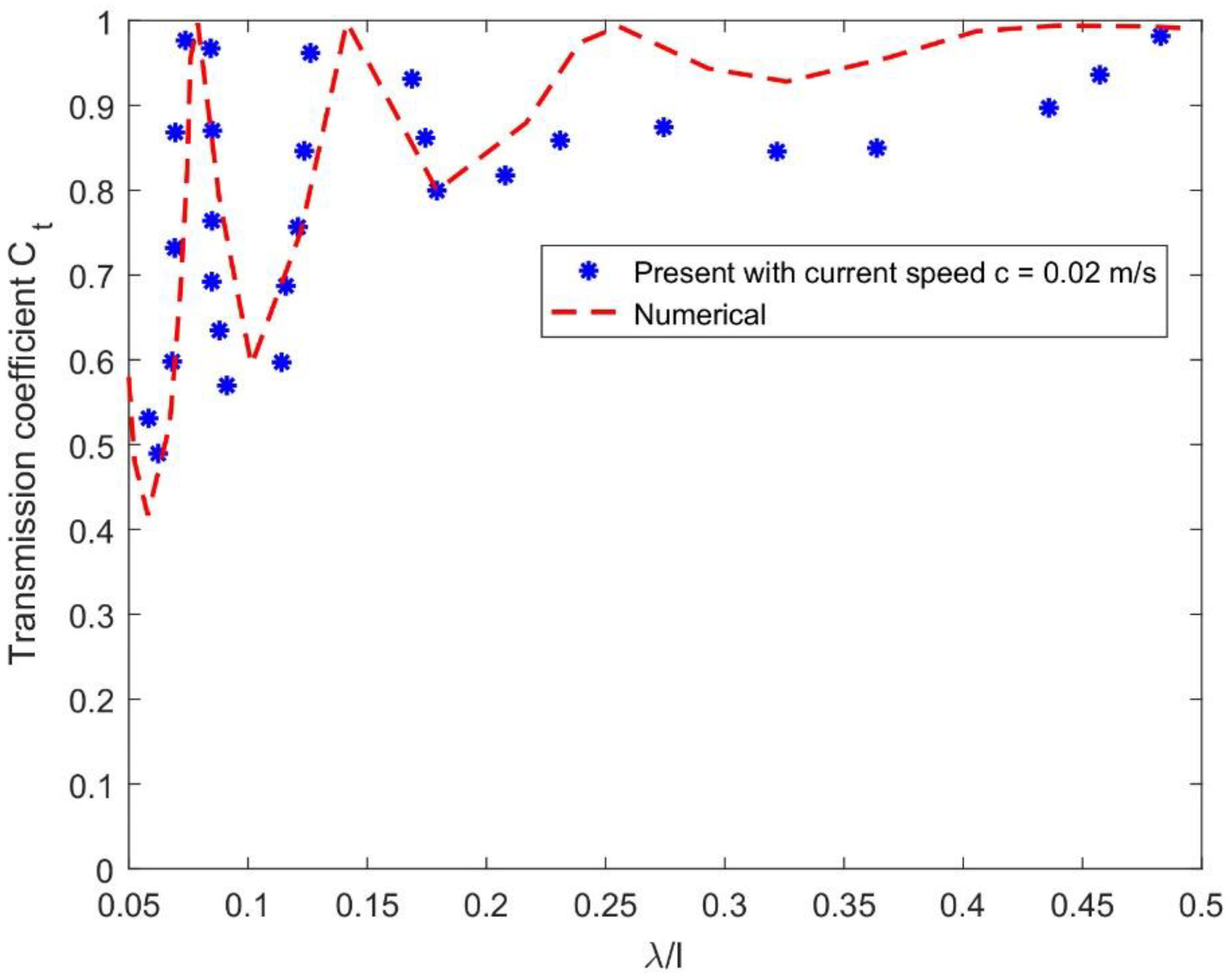
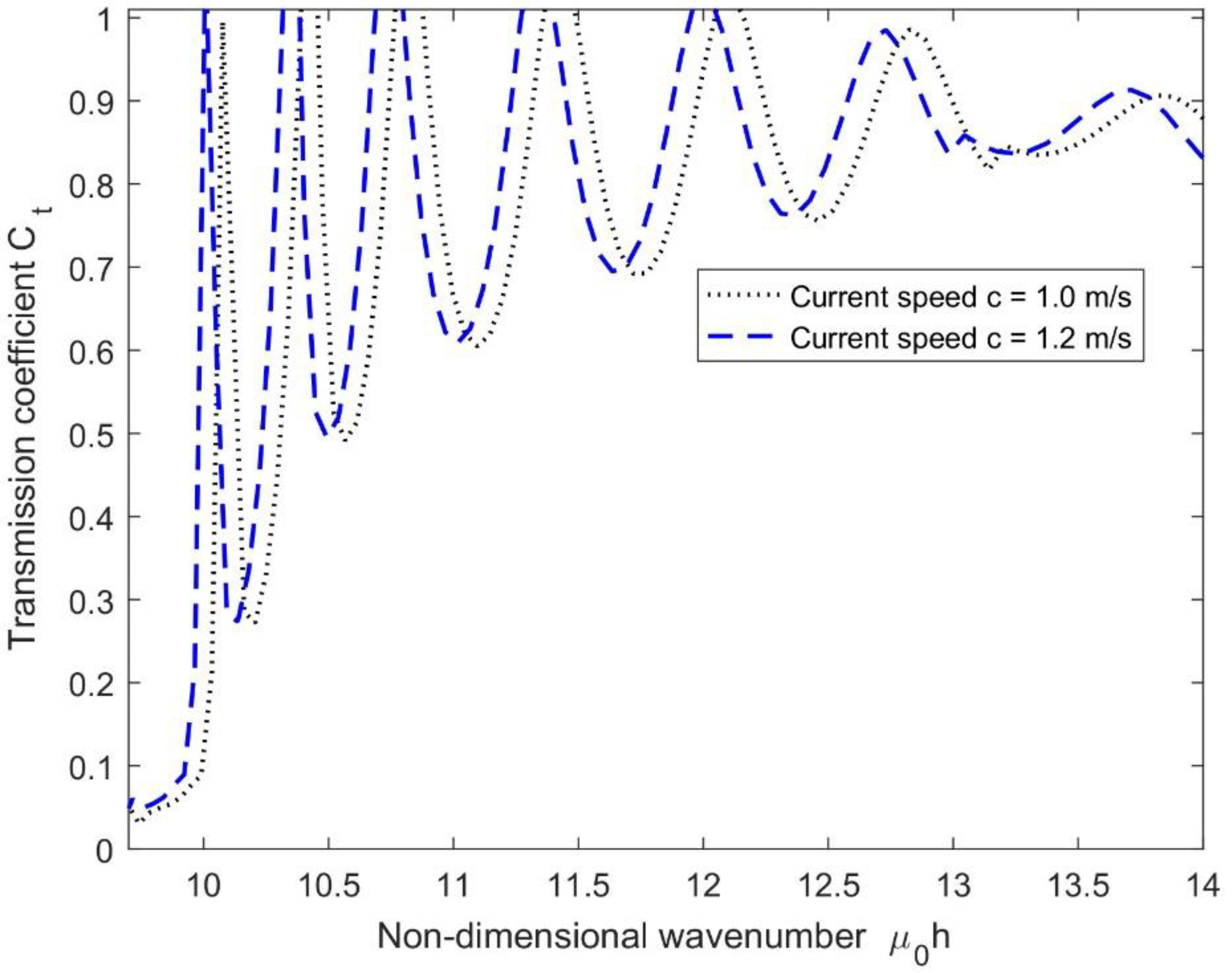
4.3. Effect of Current Speed on Transmission Coefficient

In Figure 9, the effect of different current speeds c on the transmission coefficients $C_t$ versus the non-dimensional wavenumber with the same parameter values mentioned in Table 1 is plotted. It is observed that as the current speed c increases, the transmission coefficients increase for particular values of the mooring stiffness and elastic modulus of the structure. This is because, as the current speed becomes higher, the deflection increases, which leads to more wave energy passing below the floating structure.

Figure 10 presents the variations of $C_t$ for different non-dimensional water depths $h/l$ versus non-dimensional wavenumbers ${\mu }_{0}h$ with a current speed $c=1.0 \mathrm{m}/\mathrm{s}$ and mooring stiffness $k={10}^9 \mathrm{N}/\mathrm{m}$. As can be seen, the values of $C_t$ increase with an increase in the values of $h/l$ because more wave energy passing below the floating structure leads to more transmission and less reflection in the upstream region. It is also observed that the number of resonating patterns decreases for deeper water.

Figure 11 presents the variations of $C_t$ for different mooring stiffnesses $k$ versus non-dimensional wavenumbers ${\mu }_{0}h$ with a current speed $c=1.0 \mathrm{m}/\mathrm{s}$. It can be easily seen that with an increase in the values of $k$, the values of $C_t$ decrease slightly for lower values of ${\mu }_{0}h$, which suggests that higher stiffness prevents the wave transmission that leads to lower transmission coefficients.

In Figure 12, the transmission coefficients $C_t$ for different elastic moduli $E$ versus ${\mu }_{0}h$ with a certain value of mooring stiffness $k={10}^9 \mathrm{N}/\mathrm{m}$ are plotted. In this case, the variation in $C_t$ is observed for smaller values of the non-dimensional wavenumber primarily due to an increase in rigidity of the floating structure with mooring stiffness and current speed $c=1.0 \mathrm{m}/\mathrm{s}$ that leads to higher reflection in the upstream region.

It may be mentioned that, in general, as seen in Figure 9, Figure 10, Figure 11 and Figure 12, the resonating patterns in $C_t$ occurred because of a change in phase due to the interaction of incident and reflected waves at the structural edges under the current speed with mooring lines. However, the number of resonating patterns was reduced as the non-dimensional wavenumber increased.

5. Conclusions

In this paper, a new contribution complementing previous research [37] addresses the influence of current speed on the hydroelastic response of floating flexible structures based on the Timoshenko–Mindlin beam theory in water of a finite depth. The obtained analytical result is compared with the existing published numerical results from BIEM, and the comparison between free and moored floating structures for different current speeds is also performed using the present solution. Further, the effect of the current speed along with the mooring lines’ stiffness and different design parameters is analyzed via structural displacements and transmission coefficients. From the study, it has been observed that:

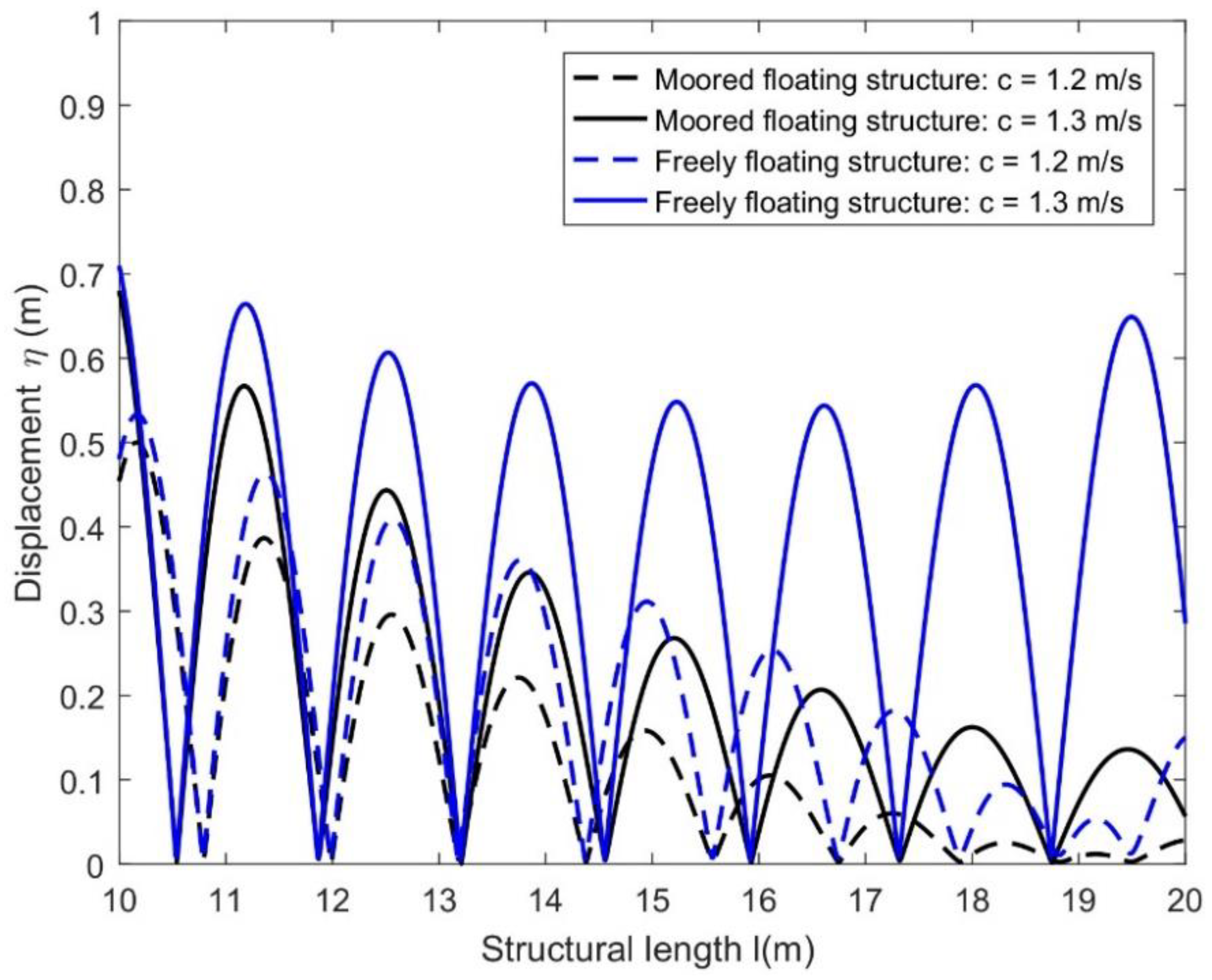
• The present result is supported by the existing numerical results published, other calculation results, and experimental datasets available in the literature, and the comparison between the moored and free-edge floating shows that the moored structure provides greater stability than that of the freely floating structure as it deflects more than that of the free one.
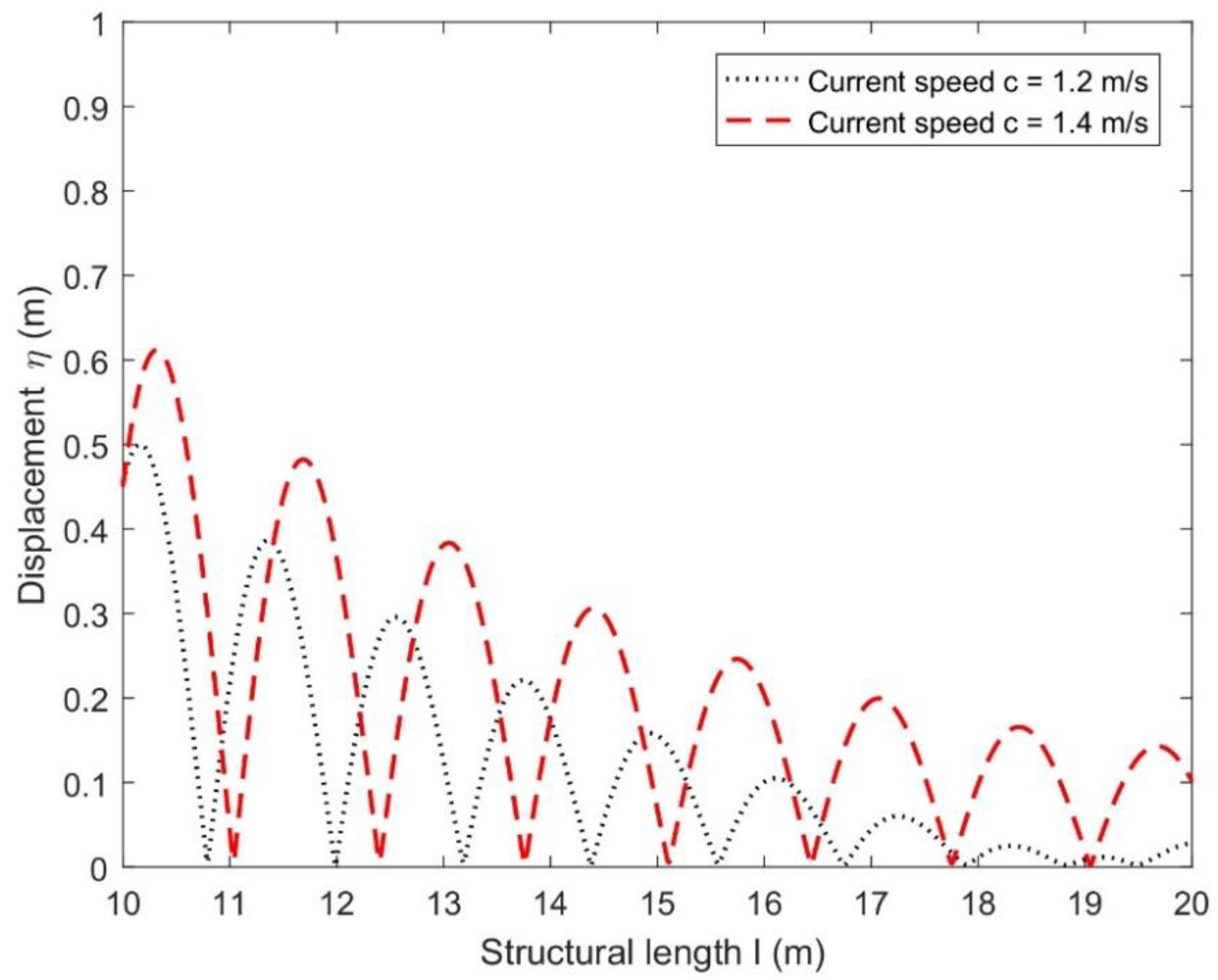
• The structural displacements increase for higher values of current speeds, which is due to the higher hydrodynamic loads on the structure in the upstream region.
• As the current speed increases, the transmission coefficients increase because the larger current provides larger hydrodynamic forces, which results in higher displacements that lead to more wave energy passing below the structure. Furthermore, the number of resonating patterns decreases as the wavenumber increases, which is expected as the wave reflection decreases in the upstream region.
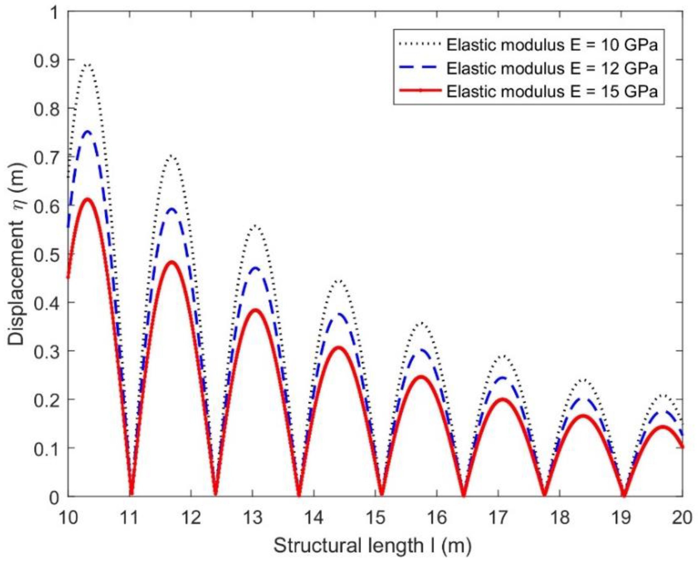
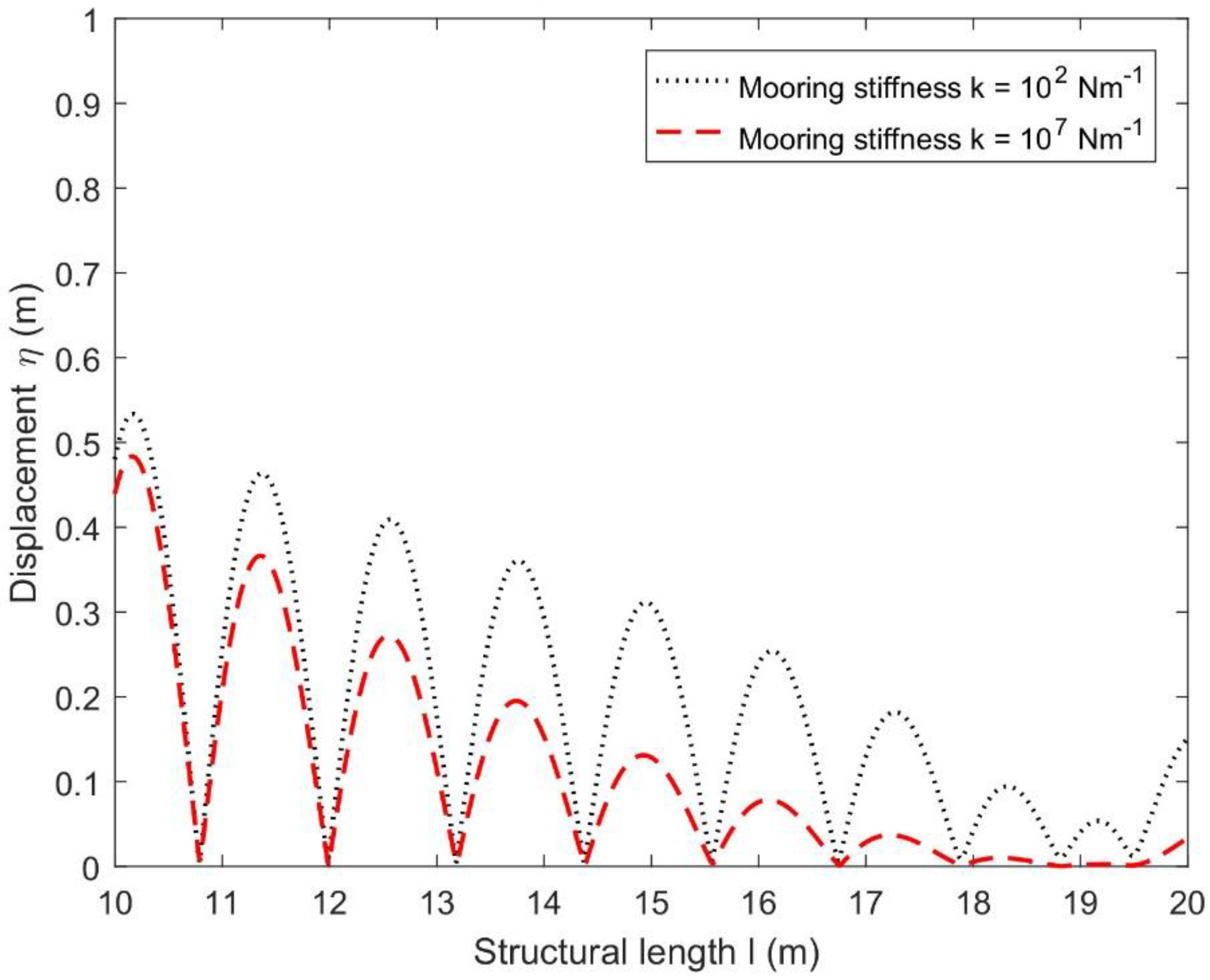
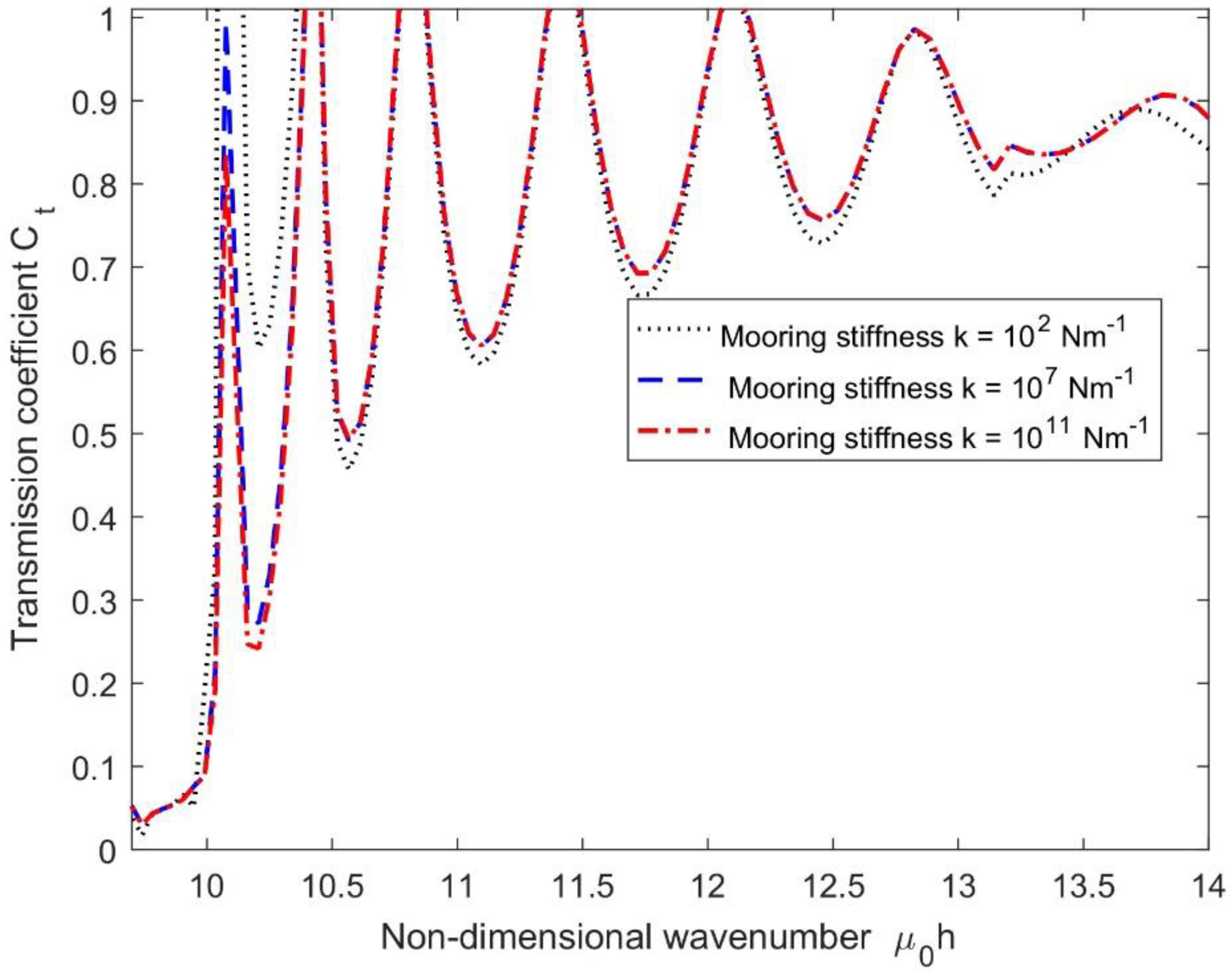
• The analysis of the structural displacements and transmission coefficients for different current speeds suggested that the floating flexible structure became more stable for lower values of current speed and higher mooring stiffness.
• Therefore, the present study indicated that the mathematical model will be helpful to develop a three-dimensional analytical model by considering the opposite current to analyse the hydroelastic response and sensitivity analysis of floating flexible structures based on the Timoshenko–Mindlin beam theory.

References

- Thomas, G.; Klopman, G. Wave-current interactions in the near shore region. Int. Ser. Adv. Fluid Mech. 1997, 10, 255. [Google Scholar]
- Miao, Y.J.; Chen, X.J.; Ye, Y.L.; Ding, J.; Huang, H. Numerical modeling and dynamic analysis of a floating bridge subjected to wave, current and moving loads. Ocean Eng. 2021, 225, 108810. [Google Scholar] [CrossRef]
- Huang, J.; Teng, B.; Cong, P.W. Wave-current interaction with three-dimensional bodies in a channel. Ocean Eng. 2022, 249, 110952. [Google Scholar] [CrossRef]
- Latheef, M.; Abdulla, N.; Faieez, M.; Jupri, M.F.M. Wave current interaction: Effect on force prediction for fixed offshore structures. In Proceedings of the International Conference on Civil, Offshore & Environmental Engineering 2018 (ICCOEE 2018), Kuala Lumpur, Malaysia, 13–14 August 2018; Volume 203, p. 01011. [Google Scholar]
- Rey, V.; Touboul, J. Forces and moment on a horizontal plate due to regular and irregular waves in the presence of current. Appl. Ocean Res. 2011, 33, 88–99. [Google Scholar] [CrossRef]
- Chen, L.; Basu, B. Wave-current interaction effects on structural responses of floating offshore wind turbines. Wind Energy 2019, 22, 327–339. [Google Scholar] [CrossRef]
- Li, Y.; Lin, M. Hydrodynamic coefficients induced by waves and currents for submerged circular cylinder. Procedia Eng. 2010, 4, 253–261. [Google Scholar] [CrossRef]
- Viuff, T.; Xiang, X.; Øiseth, O.; Leira, B.J. Model uncertainty assessment for wave- and current-induced global response of a curved floating pontoon bridge. Appl. Ocean Res. 2020, 105, 102368. [Google Scholar] [CrossRef]
- Lu, D.Q.; Yeung, R.W. Hydroelastic waves generated by point loads in a current. Int. J. Offshore Polar Eng. 2015, 25, 8–12. [Google Scholar]
- Qua, X.; Li, Y.; Tang, Y.; Hu, Z.; Zhang, P.; Yin, T. Dynamic response of spar-type floating offshore wind turbine in freak wave considering the wave-current interaction effect. Appl. Ocean Res. 2020, 100, 102178. [Google Scholar] [CrossRef]
- Zhu, T.; Ke, S.; Li, W.; Chen, J.; Yun, Y.; Ren, H. WRF-CFD/CSD analytical method of hydroelastic responses of ultra-large floating body on maritime airport under typhoon-wave-current coupling effect. Ocean Eng. 2022, 261, 112022. [Google Scholar] [CrossRef]
- Ping, W.; Yongyan, W.; Chuanqi, S.; Yanzhao, Y. Nonlinear Hydroelastic Waves Generated due to a Floating Elastic Plate in a Current. Adv. Math. Phys. 2017, 2017, 2837603. [Google Scholar]
- Bhattacharjee, J.; Sahoo, T. Interaction of current and flexural gravity waves. Ocean Eng. 2007, 34, 1505–1515. [Google Scholar] [CrossRef]
- Bispo, I.B.S.; Mohapatra, S.C.; Guedes Soares, C. Numerical analysis of a moored very large floating structure composed by a set of hinged plates. Ocean Eng. 2022, 253, 110785. [Google Scholar] [CrossRef]
- Lamas-Pardo, M.; Iglesias, G.; Carral, L. A review of Very Large Floating Structures (VLFS) for coastal and offshore uses. Ocean Eng. 2015, 109, 677–690. [Google Scholar] [CrossRef]
- Mindlin, R.D. Influence of rotary inertia and shear on flexural motion of isotropic elastic plates. J. Appl. Mech. (ASME) 1951, 18, 31–38. [Google Scholar] [CrossRef]
- Mohapatra, S.C.; Guedes Soares, C. Interaction of ocean waves with floating and submerged horizontal flexible structures in three-dimensions. Appl. Ocean Res. 2019, 83, 136–154. [Google Scholar] [CrossRef]
- Mohapatra, S.C.; Guedes Soares, C. Hydroelastic behaviour of a submerged horizontal flexible porous structure in three-dimensions. J. Fluids Struct. 2021, 104, 103319. [Google Scholar] [CrossRef]
- Mohapatra, S.C.; Guedes Soares, C. Effect of mooring lines on the hydroelastic response of a floating flexible plate using the BIEM approach. J. Mar. Sci. Eng. 2021, 9, 941. [Google Scholar] [CrossRef]
- Mohapatra, S.C.; Guedes Soares, C. Surface gravity wave interaction with a horizontal flexible floating plate and submerged flexible porous plate. Ocean Eng. 2021, 237, 109621. [Google Scholar] [CrossRef]
- Mohapatra, S.C.; Guedes Soares, C. 3D hydroelastic modelling of fluid-structure interactions of porous flexible structures. J. Fluids Struct. 2022, 112, 103588. [Google Scholar] [CrossRef]
- Papathanasiou, T.K.; Belibassakis, K.A. Hydroelastic analysis of VLFS based on a consistent coupled-mode system and FEM. IES Part A Civ. Struct. Eng. 2014, 7, 195–206. [Google Scholar] [CrossRef]
- Andrianov, A.I.; Hermans, A.J. Hydroelastic analysis of a floating plate of finite draft. Appl. Ocean Res. 2006, 28, 313–325. [Google Scholar] [CrossRef]
- Zilman, G.; Miloh, T. Hydroelastic buoyant circular plate in shallow water: A closed form solution. Appl. Ocean Res. 2000, 22, 191–198. [Google Scholar] [CrossRef]
- Watanabe, E.; Utsunomiya, T.; Wang, C.M. Hydroelastic analysis of pontoon-type VLFS: A literature survey. Eng. Struct. 2004, 26, 245–256. [Google Scholar] [CrossRef]
- Cheng, Y.; Ji, C.; Zhai, G.; Gaidai, O. Hydroelastic analysis of oblique irregular waves with a pontoon-type VLFS edged with dual inclined perforated plates. Mar. Struct. 2016, 49, 31–57. [Google Scholar] [CrossRef]
- Yoon, J.S.; Cho, S.P.; Jiwinangun, R.G.; Lee, P.S. Hydroelastic analysis of floating plates with multiple hinge connections in regular waves. Mar. Struct. 2014, 36, 65–87. [Google Scholar] [CrossRef]
- Andrianov, A.I.; Hermans, A.J. The influence of water depth on the hydroelastic response of a very large floating platform. Mar. Struct. 2003, 16, 355–371. [Google Scholar] [CrossRef]
- Karperaki, A.E.; Belibassakis, K.A. Hydroelastic analysis of Very Large Floating Structures in variable bathymetry regions by multi-modal expansions and FEM. J. Fluids Struct. 2021, 102, 103236. [Google Scholar] [CrossRef]
- Nguyen, X.V.; Luong, V.; Cao, T.N.T.; Lieu, X.Q.; Nguyen, T.B. Hydroelastic responses of floating composite plates under moving loads using a hybrid moving element-boundary element method. Adv. Struct. Eng. 2020, 23, 2759–2775. [Google Scholar] [CrossRef]
- Lamei, A.; Hayatdavoodi, M.; Wong, C.; Tang, B. On Motion and Hydroelastic analysis of a Floating Offshore Wind Turbine. In Proceedings of the ASME 2019 38th International Conference on Ocean, Offshore and Arctic Engineering, Glasgow, UK, 9–14 June 2019. Paper No. OMAE2019-96034, V010T09A070. [Google Scholar]
- Amaechi, C.V.; Reda, A.; Butler, H.O.; Ahmed Ja’e, I.; An, C. Review on Fixed and Floating Offshore Structures. Part II: Sustainable Design Approaches and Project Management. J. Mar. Sci. Eng. 2022, 10, 973. [Google Scholar] [CrossRef]
- Shumin, C.; Swamidas, A.S.J.; Sharp, J.J. Similarity method for modelling hydroelastic offshore platforms. Ocean Eng. 1996, 23, 575–595. [Google Scholar] [CrossRef]
- Fu, S.; Moan, T.; Chen, X.; Cui, W. Hydroelastic analysis of flexible floating interconnected structures. Ocean Eng. 2007, 34, 1516–1531. [Google Scholar] [CrossRef]
- Ruzzo, C.; Failla, G.; Arena, F.; Collu, M.; Li, L.; Mariotti, C. Analysis of The Coupled Dynamics of an Offshore Floating Multi-Purpose Platform, Part B: Hydro-Elastic Analysis with Flexible Support Platform. In Proceedings of the ASME 2019 38th International Conference on Ocean, Offshore and Arctic Engineering, OMAE2019, Glasgow, Scotland, 9–14 June 2019. [Google Scholar]
- Kang, H.; Kim, M. Hydroelastic analysis and statistical assessment of flexible offshore platforms. Int. J. Offshore Polar Eng. 2014, 24, 35–44. [Google Scholar]
- Amouzadrad, P.; Mohapatra, S.C.; Guedes Soares, C. Hydroelastic response of a moored floating flexible offshore structure based on Timoshenko-Mindlin-Beam theory. In Trends in Renewable Energies Offshore, 1st ed.; Soares, G., Ed.; Taylor & Francis Group: London, UK, 2022; pp. 879–887. ISBN 9781003360773. [Google Scholar]
- Tay, Z.Y.; Wang, C.M. Reducing hydroelastic response of very large floating structures by altering their plan shapes. Ocean Syst. Eng. 2012, 2, 69–81. [Google Scholar] [CrossRef]
- Zhao, C.; Hu, C.; Wei, Y.; Zhang, J.; Huang, W. Diffraction of surface waves by floating elastic plates. J. Fluids Struct. 2008, 24, 231–249. [Google Scholar] [CrossRef]
- Loukogeorgaki, E.; Yagci, O.; Sedat Kabdasli, M. 3D Experimental investigation of the structural response and the effectiveness of a moored floating breakwater with flexibly connected modules. Coast. Eng. 2014, 91, 164–180. [Google Scholar] [CrossRef]
- Vengatesan, V.; Varyani, K.S.; Westlake, P.C. Drag and inertia coefficients for horizontally submerged rectangular cylinders in waves and currents. J. Eng. Marit. Environ. Part M 2009, 223, 121–136. [Google Scholar]
- Dai, J.; Abrahamsen, B.C.; Viuff, T.; Leira, B.J. Effect of wave-current interaction on a long fjord-crossing floating pontoon bridge. Eng. Struct. 2022, 266, 114549. [Google Scholar] [CrossRef]
- Liu, Z.; Mohapatra, S.C.; Guedes Soares, C. Finite Element Analysis of the Effect of Currents on the Dynamics of a Moored Flexible Cylindrical Net Cage. J. Mar. Sci. Eng. 2021, 9, 43. [Google Scholar]
- Wu, C.; Watanabe, E.; Utsunomiya, T. An eigenfunction expansion-matching method for analyzing the wave-induced responses of an elastic floating plate. Appl. Ocean Res. 1995, 17, 301–310. [Google Scholar] [CrossRef]
- Utsunomiya, T.; Watanabe, E.; Wu, C.; Hayashi, N.; Nakai, K.; Sekita, K. Wave Response Analysis of a Flexible Floating Structure By BE-FE Combination Method. In Proceedings of the Fifth International Offshore and Polar Engineering Conference, The Hague, The Netherlands, 11 June 1995. [Google Scholar]