1. Introduction
Small floating target detections on the sea surface [
1] remain a hotspot in radar detection at home and abroad. As backscattered radar signal returns from the sea surface, sea clutter has complex characteristics such as non-uniform, non-Gaussian, non-stationary, etc. Small floating targets such as boats, frogmen, and buoys are often hidden in sea clutter and difficult to detect because of their small radar cross-section (RCS) and weak radar returns. For those traditional detection methods based on general statistical characteristics or radar returns’ energy, it is hard to maintain high detection accuracy and low false alarm rate [
2]. Accordingly, various obstacles exist in current detection technology.
At present, various feature extraction-based detection methods are proposed, including three categories. The first category is fractal characteristics-based detection method. From a non-energy perspective, fractal-based methods detect sea clutter and mine the data fractal features [
3,
4,
5]. Haykin et al. uses fractal dimension characteristics of sea clutter to detect small floating targets in the earlier time [
6]. Subsequently, the differences between sea clutter and target returns are also used for detection in terms of their single-scale fractal dimension features [
7]. However, the fractal feature is single-dimensioned and requires a long observation time. Later on, detection methods to extract multifractal parameters are gradually developed. The second category is time–frequency (TF)-based detection methods. Based on signal TF information, TF-based methods map the original data to the TF distribution spaces, and then extract relevant features [
8,
9,
10,
11]. TF method is thus widely used in the sea clutter field effective for non-linear and non-stationary complex signals. Shui et al. constructs a three-feature detector which selects relative amplitude features from the time domain, relative Doppler peak height and relative vector entropy features from the frequency domain [
12]. As an improvement to [
12], three TF features are re-extracted, which greatly improves their detection performances [
13]. The third category is machine learning (ML) algorithm-based detection methods. ML algorithms such as the traditional support vector machine (SVM) and long-short term memory (LSTM) have been verified to be able to efficiently process data [
14,
15]. As deep learning-based detection methods adaptively extract multi-dimensional signal features through neural networks and exploit deeper information of the mined signals, a convolutional neural network is adopted to realize the sea clutter and noise classification, and to carry out a refined sea clutter suppression [
16]. Since a neural network is a non-linear training process, extracted features display better discrimination and generalization. In addition, there are other target detection methods based on feature extraction. The graph connectivity density is calculated in [
17,
18], and whether the signal contains a target is judged by this single feature. Energy information is also frequently used as a feature in target detection. Shi et al. employs empirical mode decomposition (EMD) in [
19] to decompose the signal into multiple intrinsic mode function (IMF) components, and the target existence is judged by the proportion of IMF components in the original signal energy. Utilizing a single feature for detection, though different from each other, these methods naturally miss some key representations in target signal detection.
In order to extract features more effectively, the one-dimensional time series are transformed into a two-dimensional matrix in different ways. This matrix must contain a strong mapping relationship with the original signal. As a case in point, the covariance matrix well reflects the correlation of the time series, statistics are constructed according to the eigenvalues of the covariance matrix and the statistical distribution is tested for an effective target detection [
20]. Another dimension transformation method, the Grammian Angular Field (GAF), introduces a penalty inner product, which better suppresses Gaussian noise [
21]. In addition, the TFD spectrogram generated by short-time Fourier transform (STFT) is also regarded as a two-dimensional image presented under dimension transformation. As the embodiment of signal energy, the spectrogram effectively indicates signal characteristics due to its non-negativity and good suppression of cross-terms [
22,
23].
Due to the dimension transformation processing of the original time series, some image processing methods are adopted for their convenience and efficiency in recent years. Different from image matching, the key to distinguish sea clutter from target returns is matching points’ amplitude and gratitude information, while the specific position information is discarded. A symmetric positive definite (SPD) matrix of Riemannian manifold is introduced to map the 2D spectrogram to the Riemann space in [
24]. The SIFT descriptor is then used to extract 128 dimensional features containing gradient information, while the domain of sea clutter and target returns is divided by calculating the Riemann distance. However, an ensuing problem of increased calculation time emerges. The cumbersome calculation workload calls for a network simplification. Because Features from Accelerated Segment Test (FAST) algorithm excels for its convenience and speed, this paper uses FAST to extract the necessary multi-dimensional features.
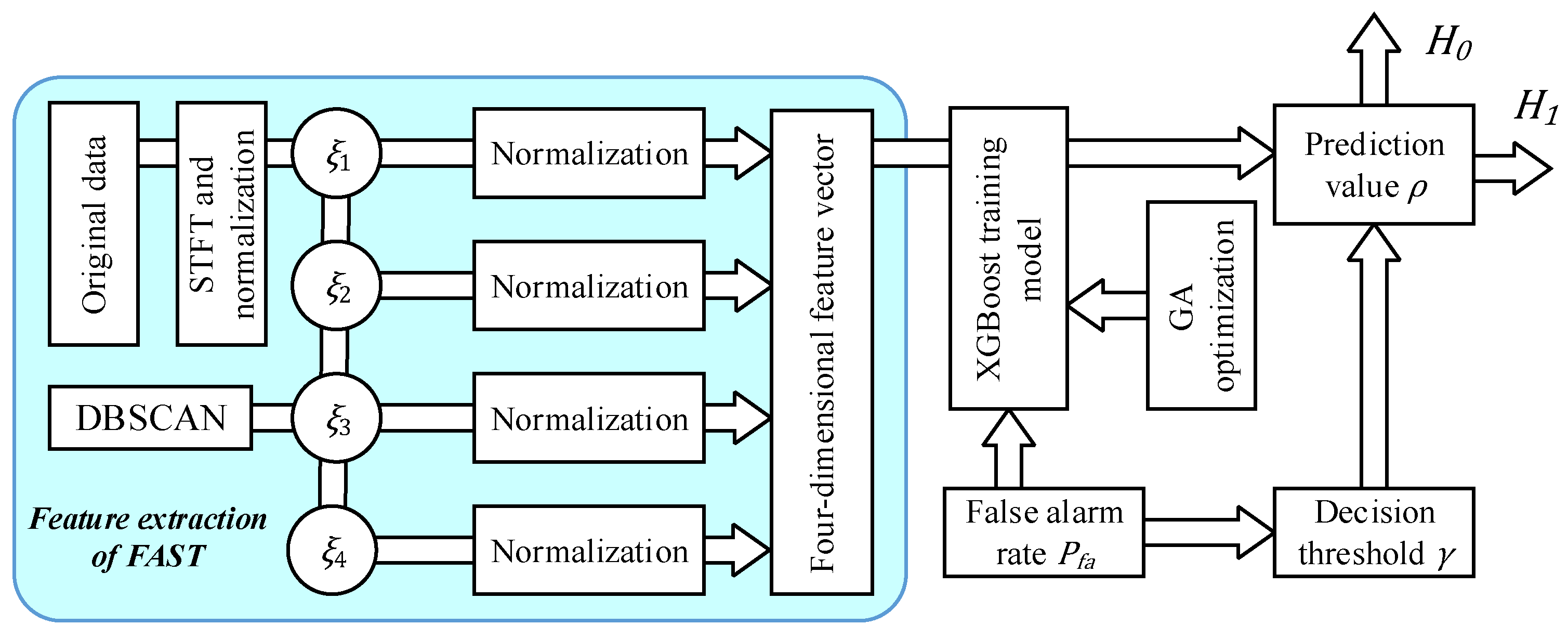
The following is the general flow of the proposed method. This paper performs short-time Fourier transform (STFT) on the original data and generates a TF distribution spectrogram. Four features are then extracted in sequence in this research. It uses FAST to extract the candidate feature points in the TF distribution spectrogram as the first overall feature. The second feature is obtained by computing the average distributed energy of all CFPs. Density-Based Spatial Clustering of Applications with Noise (DBSCAN) algorithm is used to divide clusters to constitute the third feature. Finally, the cluster with the largest number of CFPs is selected, and the number of CFP is used as the fourth feature. In order to reduce the impact of abnormal CFPs on the feature distinguishability and standardize the process, the resulted four features are optimized first, followed by a normalization process, and a four-dimensional feature space is accordingly constructed. What follows in this paper is the use of the XGBoost algorithm as the classifier, and the introduction of the genetic algorithm to optimize the hyperparameter group in XGBoost. The judgment threshold is updated in real time, according to the predicted value output by XGBoost, so as to realize a controllable false alarm rate of the detection method. A detection method based on four FAST-induced features is proposed, and the IPIX dataset is used to verify the advantage and stability in the detection performance of the proposed method.
2. Theoretical Basis of Feature Extraction
The first thing to consider in feature extraction-based target detection is actually the issue of combining general features into feature vectors and a reasonable division of the vector spaces. The target detection problem thus undergoes a transformation. Based on an effective characterization of data energy information by the spectrogram and an excellent performance of FAST algorithm for CFPs, four features are extracted and optimized in this paper. There is a detailed description concerning the transformation, feature extraction and optimization.
2.1. Target Detection Problem Transformation
It is assumed that
N consecutive pulses received by the radar constitute the original observation data
. In this way, a small target detection problem on the sea surface is transformed into a hypothesis testing issue:
where
e is the target returns and
c is the pure sea clutter. When the original observation data contain only pure sea clutter, i.e., there is no observation target, it is judged as
hypothesis. When the original observation data contain target returns, i.e., there may be an observation target here, it is judged as
hypothesis. Thus, the target detection problem is transformed into a binary classification. The design focus of the feature extraction detection is to improve the distinction between different features, divide feature vectors into different domains, and set decision thresholds.
2.2. Short-Time Fourier Transform
Due to the complex characteristics of sea clutter, it is hard to achieve high detection accuracy with a multi-dimensional feature extraction from a single domain. As an improvement, on the basis of Fourier transform, the short-time Fourier transform (STFT) then introduces the window function, which offers a limited support in the time–frequency domain. Therefore, STFT is used to realize the time–frequency signal positioning. At the same time, STFT has a strong anti-interference, and a strong capability of processing frequency-domain diversity signals, while it does not generate cross-interference terms. STFT is used to transform the original signals into a time–frequency distribution matrix, whose formula is
A modulo operation on the time–frequency distribution matrix is performed to obtain a time–frequency distribution spectrogram
A time–frequency distribution spectrogram is obtained by (3). The spectrogram has constant positivity and contains all real numbers. Since any window function satisfies
, it can be inferred that
It is clear from (4) that the spectrogram is actually a signal energy distribution. Converting the original signal into a time–frequency distribution spectrogram effectively provides the signal energy information. The time–frequency distribution spectrogram is rasterized, where the spectrogram is divided into n points and l points from the horizontal and vertical directions, respectively corresponding to the time domain axis and frequency domain axis of the spectrogram. Therefore,
is converted into
, correspondingly. Next, the spectrogram is normalized, and its normalization formula is defined as
The normalization process means that when the detection signal is pure sea clutter time series, it is a random process with zero mean and unit variance in the normalized spectrogram. By contrast, when the detection signal contains the target returns, there are obvious relevant differences between this signal and the normalized spectrogram of pure sea clutter [
10]. The formulas for the mean function
and the standard deviation function
are as follows:
2.3. Feature Extraction Based on FAST Algorithm
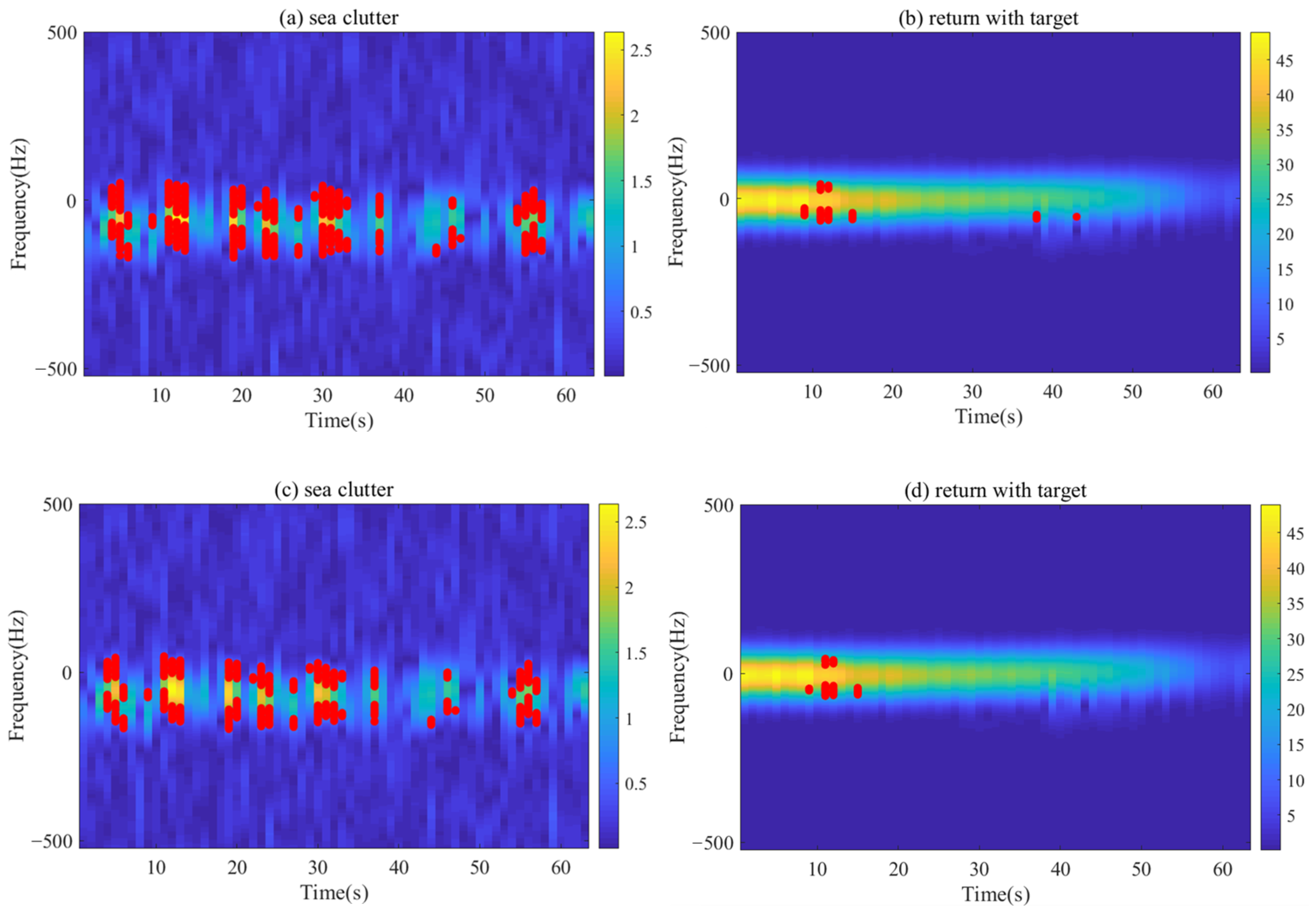
Due to the non-uniform, non-Gaussian and non-stationary characteristics of sea clutter, it is difficult to reconstruct complex sea clutter signals with simple mathematical models. Therefore, it is difficult to achieve optimum detection results with traditional single-feature based detection methods. After generating the time–frequency distribution spectrogram, the FAST algorithm is used to extract four features in the spectrogram. Specific extraction methods of the four features are given below.
As a feature point detection algorithm [
25,
26], FAST selects a
square space in the image and draws a circle in this square at its center point with a radius of 3.4. FAST, then, respectively, compares the pixel values of the center point and 16 points that the circle passes. This is followed by a pixel value subtraction by the center point to the above-mentioned 16 points. Among the subtraction differences, if there are more than 12 values greater than the set threshold
, the center point is considered as a candidate feature point (CFP). When FAST algorithm is introduced for feature extraction, the time–frequency distribution spectrogram converted from the original signal becomes the image to be further extracted. The energy value corresponding to each point in the spectrogram becomes the pixel value to be compared in the FAST algorithm. The CFPs extracted by the FAST algorithm are considered as the edge points of their respective energy peaks. The feature points detected by FAST algorithm contain only location information and are still unfit for direct target detection effectively [
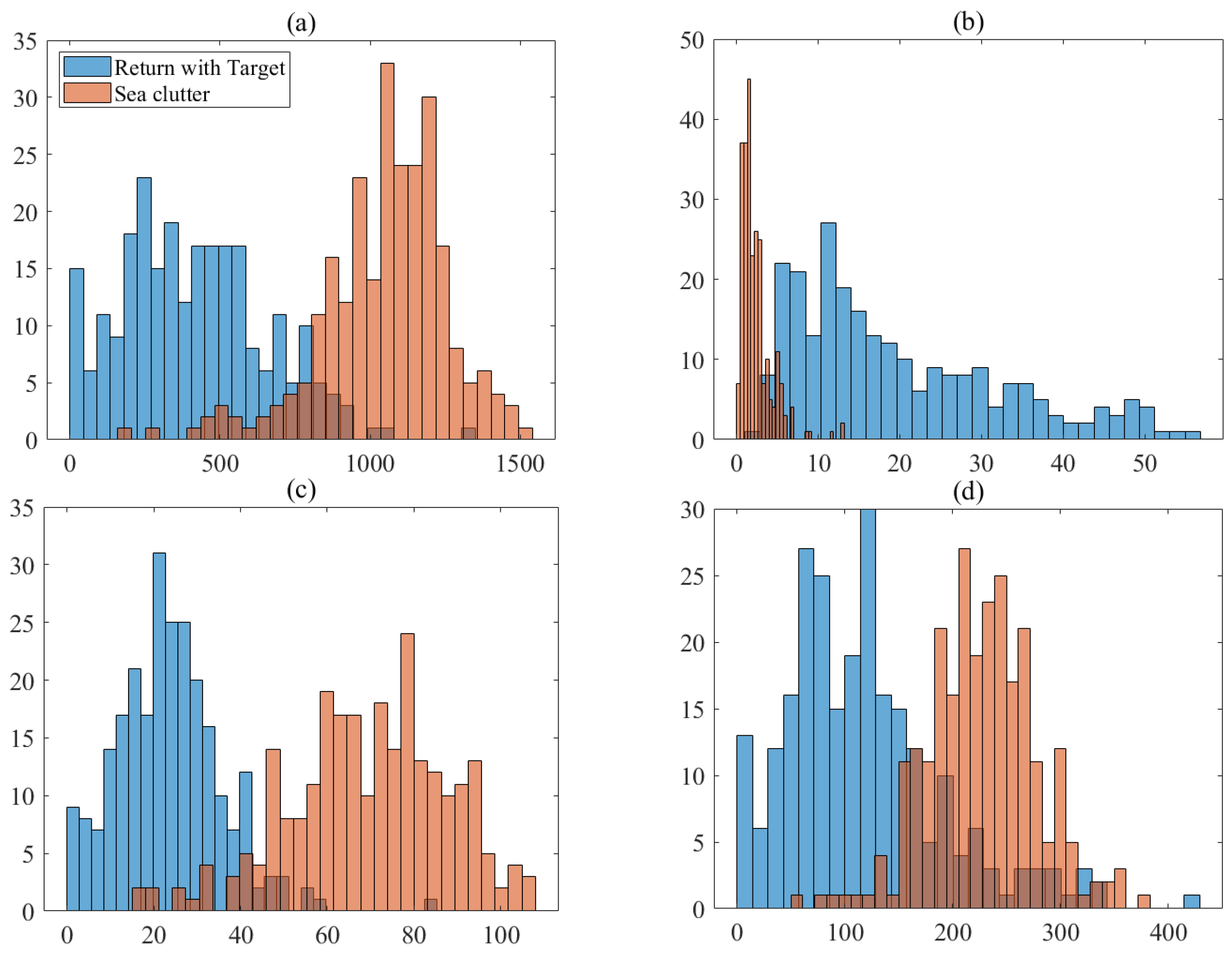
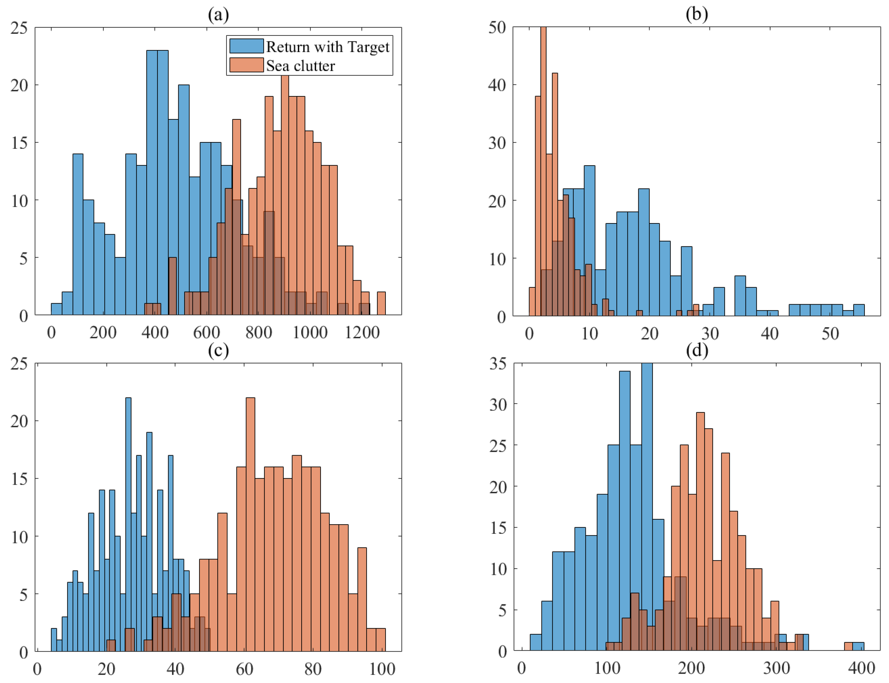
27]. This paper counts the following feature values including the number of CFPs, energy quantities, the number of clusters obtained and the number of CFPs in the largest cluster:
the number of CFPs in the time–frequency distribution spectrogram;
: average distribution energy quantity of CFPs;
: the number of clusters obtained by clustering CFPs;
: the number of CFPs in the largest cluster.
Among them, is directly obtained by the FAST algorithm to count the CFPs. is calculated from in the original spectrogram. DBSCAN algorithm is used to calculate . is obtained by selecting the cluster with the largest CFP number among all the clusters in , and then taking the number of CFPs in this newly obtained cluster as its value.
Here is a brief description of the clustering algorithm. Density-Based Spatial Clustering of Applications with Noise (DBSCAN) is an unsupervised ML clustering algorithm [
28]. It is necessary to first manually set its two key parameters. One parameter is the maximum scanning radius
, while the other is the minimum number of included points
. A point is regarded as a core point if there are more than or equal to
points within the radius
of this point. A point is regarded as a boundary point if it is not a core point and is located in the radius
of a core point. A point is regarded as a noise point if it is not located in the radius
of any core point. The calculation now begins with
and
manual setting, and then a random CFP selection. All corresponding core points and boundary points are aggregated into the same cluster, and the noise points are removed.
A CFP picking is obligatory since the energy quantity of some CFPs may be too high or too low with primary CFP extraction, resulting in a serious impact on
, and thus the final detection accuracy. All the CFPs are arranged in ascending order of energy, and then the first one-eighth and the last one-eighth of the CFPs are removed, which eliminates the influence of abnormal CFPs and optimizes each feature. Then, the four features are normalized, for different features have different value ranges. Therefore, for the
i-th feature and the obtained P four-feature samples, the calculation formula is as follows:
A four-dimensional feature space is constructed taking each feature as a dimension, thereby a four-dimensional space vector is obtained as
The obtained four-dimensional vector effectively reflects the difference between the pure sea clutter and the target returns in the time–frequency distribution, which is beneficial to the subsequent target detection process.
3. Small Target Detection on Sea Surface Based on Four FAST Features
A confusion matrix is usually used to judge feature extraction-based target detection method. The detection probability and the false alarm rate are commonly used parameters. The detection probability is the proportion of correctly judged samples among all actually targeted samples. The false alarm rate is the proportion of wrongly judged samples among all actually untargeted samples. A false alarm rate increase will lead to the network judgment imbalance, and it needs to be considered to control the false alarm rate continuously. The target detection requirement for the false alarm rate is no more than . Since the detection probability and the false alarm rate are calculated based on the same confusion matrix, they are mutually checked and balanced. A lower false alarm rate results in a lower detection probability. Therefore, the classifier’s detection probability with a constant low false alarm rate is the criterion for judging the classifier’s target detection effect.
In order to realize data classification and detection of sea cluster and target returns as well as real-time false alarm controllability, this XGBoost classifier is optimized first to make up for its previous inadequacy as illustrated in relevant studies. Then, optimized XGBoost algorithm classifies the extracted four-dimensional feature vectors. So far, combining the FAST-based feature extraction with the optimized XGBoost classifier, this paper proposes a FAST four-feature based small target detection method on the sea surface and elaborates the detection results.
3.1. XGBoost Classifier
Most of the currently adopted methods, such as support vector machine (SVM) [
29], linear regression (LR) [
30], and decision tree (DT) [
31], are implemented for a binary classification, but they are unable to guarantee fairly accurate detection results for uncontrollable false alarms. Therefore, this paper chooses the XGBoost algorithm to construct the classifier, which is a multi-class regression tree ensemble algorithm combining multiple different decision tree models into a relatively better model [
32]. The model formula is
where
is the predicted value of the model for samples after
iterations,
is the total number of trees.
is a function in the function space
,
is the i-th sample of the input data,
is the prediction result of the first
t-1 trees, and
is the model of the
t-th tree. Since XGBoost adopts a gradient boosting strategy, each new decision tree added in the training process gradually fits the previous total learning error, thus ensuring a better training effect. The objective function of the XGBoost algorithm is
where
is the loss function,
is the real sample value,
is the regular term calculated by all decision trees, and
is a constant. One of XGBoost advantages lies in its expansion of the objective function with a second-order Taylor function, which is
where
and
are the first derivative and the second derivative after expansion, respectively. All the samples
of the
j-th leaf node are classified into the sample set of a leaf node, defined as
; then. formula (12) is rewritten as
Among these,
is the influence coefficient,
is the
regularization coefficient,
is the number of leaf nodes of the current tree, and
is the weight value of the leaf node. Let the derivative of the objective function be zero; the optimal weight is obtained, and the final objective function is
where the tree construction plays a key role. The parameters of a decision tree are called hyperparameters. The hyperparameter optimization process and the controllable implementation method of false alarms are described in detail below.
3.2. XGBoost Hyperparameter Optimization and False Alarm Rate Controlling
The training results of the XGBoost algorithm are affected by the hyperparameters in the model.
Table 1 shows some of XGBoost hyperparameters and their default values. An improper selection of hyperparameter values seriously affects detection results and then detection accuracies. Therefore, genetic algorithm (GA) is used to first optimize the four hyperparameters listed in
Table 1 [
33]. A total of 50 randomly generated hyperparameter groups are set, and the values of all hyperparameter groups are converted into binary codes. After group selection, crossover, mutation and elimination, a new hyperparameter group value is obtained, and the detection probability is used as a GA fitness function. After the above multiple iteration, it is taken as the condition for the iteration termination whether the difference between the highest and lowest fitness value is less than
. Finally, the original model obtains the optimal hyperparameter group and an optimized XGBoost model most suitable for the training samples.
After training with this optimized XGBoost model, the predicted value
corresponding to each group of four-dimensional feature vectors is obtained. In order to realize the false alarm controllability, all predicted values that are actually sea clutter samples are picked up, denoted as
. When the false alarm rate is set, the decision threshold
is calculated:
Then, it compares all the predicted values with the decision threshold. If
, it is judged not to contain the target echo and it belongs to
hypothesis. If
, it is judged as to contain the target echo and it belongs to
hypothesis. The detection probability is calculated according to the judgment results, with a controlled false alarm rate [
34,
35]. In GA iterative process, the prediction values obtained from each group training with different hyperparameters are calculated according to (15) to update the decision threshold, so as to effectively realize a real-time control of the false alarm rate.
3.3. Detection Method Based on Four FAST Features
Combining the FAST-based feature extraction with the optimized XGBoost classifier, the FAST four-feature (FAST-4F) detection method is proposed. The flowchart is illustrated in
Figure 1. First, the IPIX dataset is used as original data, whose detailed description is given below in Period 4. The original data are converted into a TF distribution spectrogram using the STFT, and then the TF distribution spectrogram is normalized. The FAST algorithm extracts CFPs in the spectrogram and the CFPs are counted as
, which is used to calculate
. DBSCAN is used to divide clusters and count them as
, which finally results in
. Next, the four features are further normalized and unified, so as to construct a four-dimensional feature vector. So far, the feature extraction finishes.
What follows is the classification detection procedure, where XGBoost training model is used to perform binary classification on the constructed four-dimensional feature vector. GA is used to optimize the hyperparameters in the XGBoost training model. The decision threshold is obtained by taking the false alarm rate into account. The prediction value obtained by the XGBoost training model is compared with to obtain the final classification result.
5. Conclusions
This paper first performs STFT on the original data to generate a TF distribution spectrogram. FAST algorithm is used to extract the CFPs in the TF distribution spectrogram as the first feature . is calculated by . DBSCAN is used to divide clusters and count them as , which finally results in . In order to enhance the distinction between sea clutter and target returns, the four features are picked up. According to CFP energy sequencing from small to large, the first and the last one-eighth of the CFPs are removed, and re-statistics are performed. Then, feature normalization is performed and a four-dimensional feature space is constructed. XGBoost algorithm is used as the classifier, and GA is introduced to optimize the hyperparameters in XGBoost. The judgment threshold is updated in real time according to the prediction value output by XGBoost, which controls classifiers’ false alarm rates.
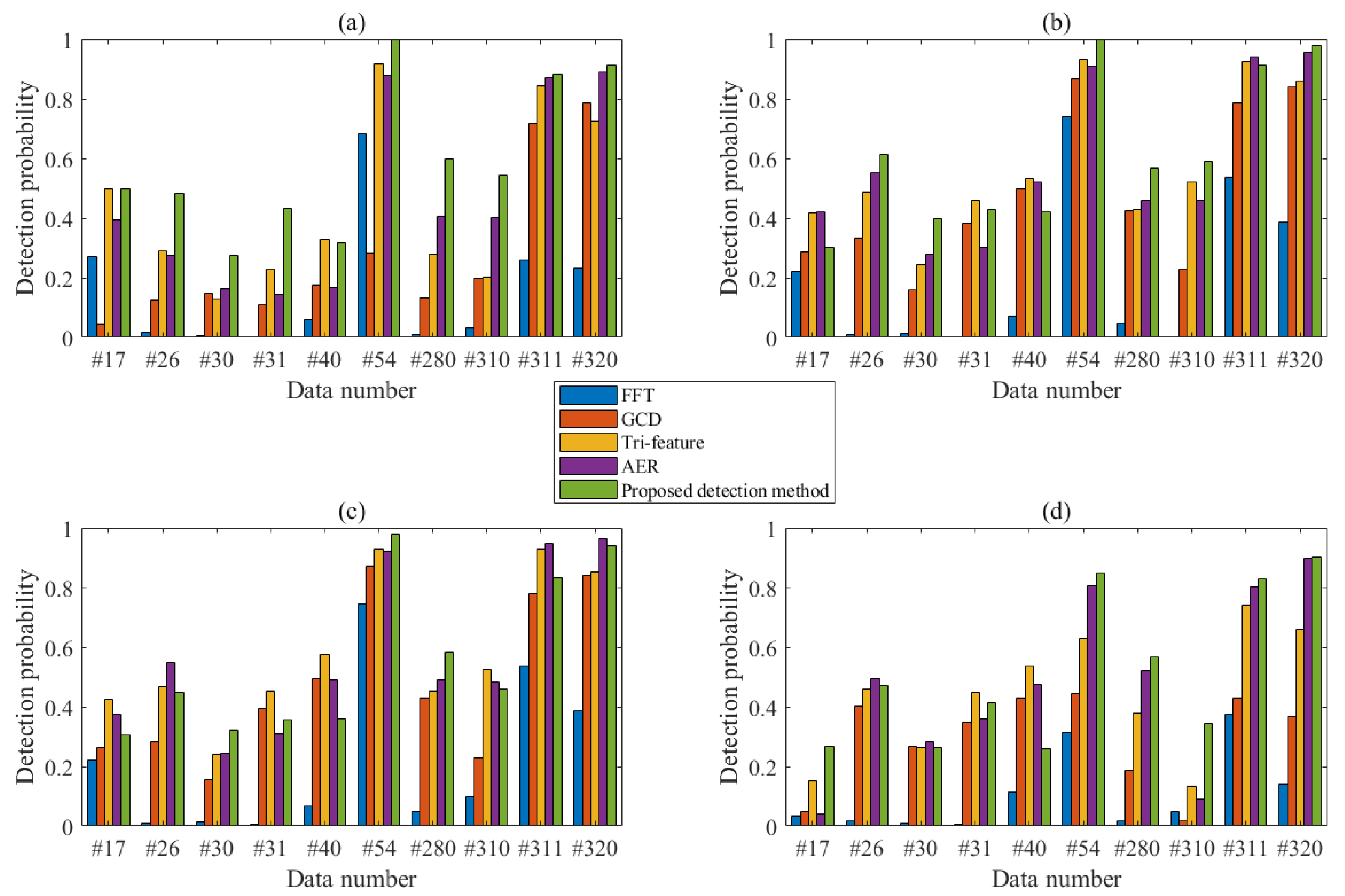
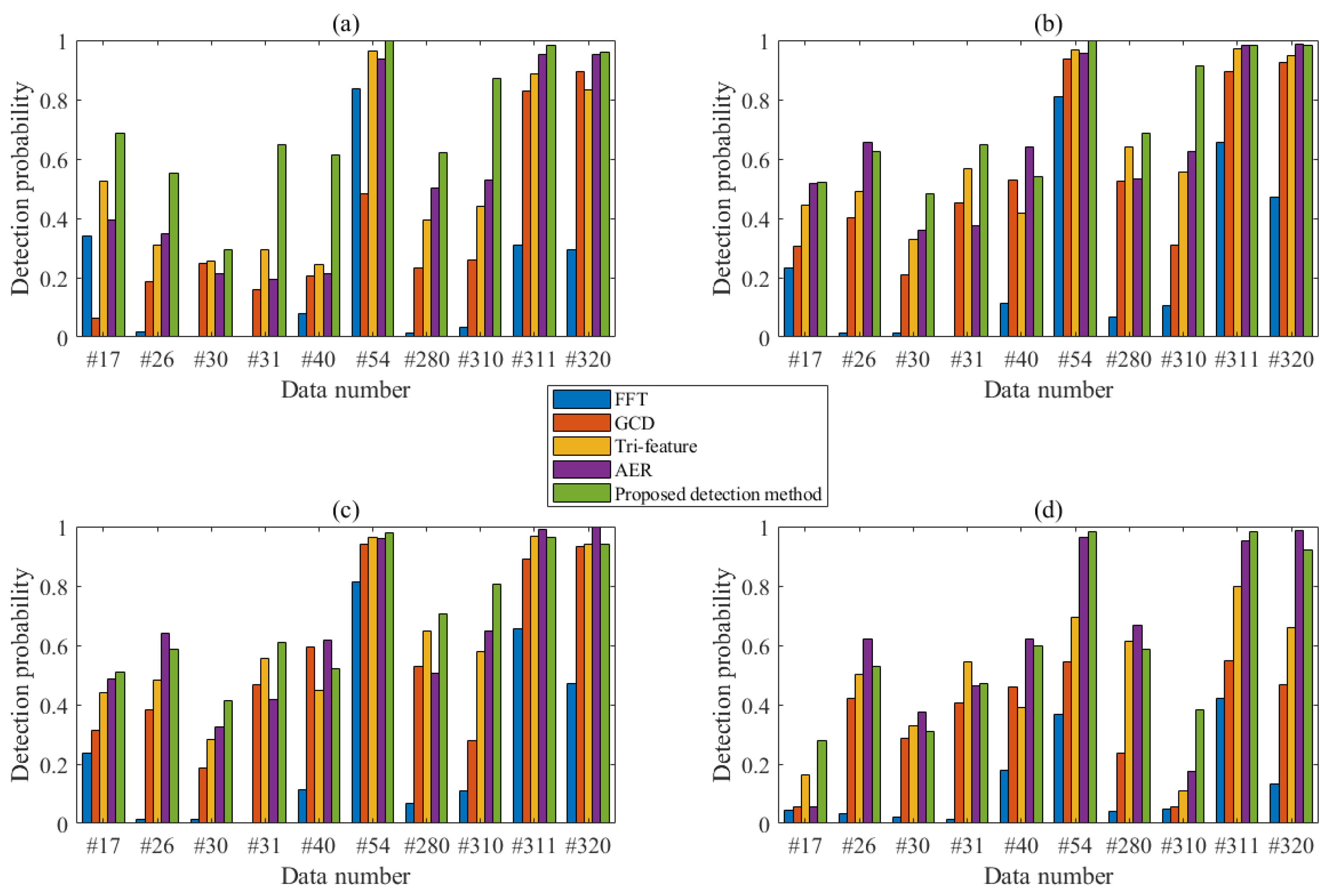
A FAST-4F detection method is proposed and verified with IPIX dataset. The experimental results show that proposed detection method has excellent detection performance. Compared with several currently existing detection methods, when N = 512, the FAST-4F is superior to other detection methods, and its performance is improved by more than 7%. When N = 1024, the performance of proposed detection method is improved by 13.8%. In summary, the FAST four-feature detection method has a good detection performance, a simple model and a fast calculation, and therefore is ready to be applied to the small target detections on the sea surface.
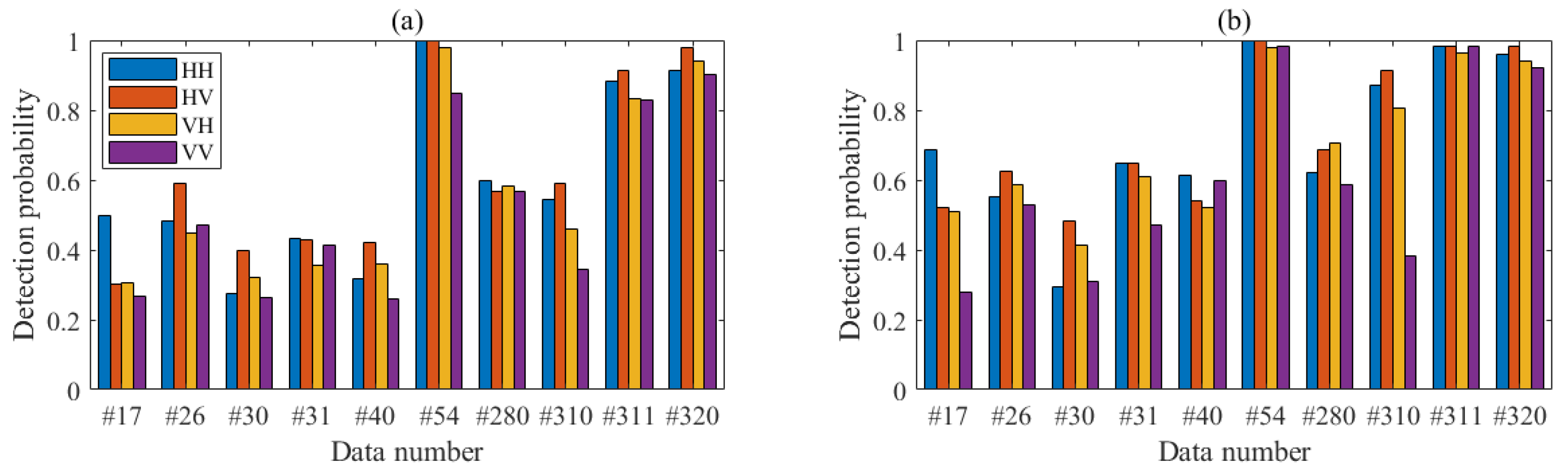
The detection method proposed in this paper still has some limitations. For example, TFD spectrograms manifest different distribution characteristics at different polarizations. Later studies may focus on TFD improvements for smoother and clearer two-dimensional images. In addition, this paper adopts a manual set of parameters in each algorithm. There is great room for more adaptive methods to improve its practicability so as to achieve a clearer and generalization ability. This section is not mandatory but can be added to the manuscript if the discussion is unusually long or complex.


 ,
, 
