Abstract
Biomass is a renewable energy source because it is contained in organic material such as plants. This paper introduces a modified hunger games search for solving global optimization and biomass distributed generator problems. The hunger search algorithm is a very recent optimization algorithm. Despite its merits, it still needs some modifications. The proposed approach includes a new binary τ-based crossover strategy with satisfaction fulfillment step mechanisms. This new algorithm is designed to improve the original hunger games search algorithm by addressing some of its shortcomings, specifically, in solving problems related to global optimization such as finding the best possible solutions for biomass distributed generators. To assess the power of the new approach, its performance was evaluated on the IEEE CEC’2020 test suite against five recent and competitive algorithms. This comparison process included applying the Wilcoxon sign rank and Friedman statistical tests. Reducing the system losses and enhancing the network’s voltage profile are two main issues in the stability of radial distribution networks. Optimal allocation of biomass distributed generators in radial distribution networks can not only improve their stability but also guarantee good service to the customers. Consequently, this research work suggests an effective strategy based on the proposed approach to produce the optimal positions, sizes, and power factors of the biomass distributed generators in the network. Accordingly, the target is to mitigate the network’s active power loss such that the power flow and the bus voltage have to be maintained at their standard limits. Three distribution networks were considered for validating the superiority of the new proposed algorithm. These networks are the IEEE 33-bus, IEEE 69-bus, and IEEE 119-bus. The obtained results were compared with the gravitational search algorithm, whale optimization algorithm, grey wolf optimizer, Runge Kutta method, and the original hunger search algorithm. The new approach outperformed the other considered approaches in obtaining the optimal parameters, which mitigated the power loss to 11.6300, 5.2291, and 145.489 kW, with loss reduction of 94.49%, 97.68%, and 88.79% for the three networks, respectively.
1. Introduction
Nowadays, everybody who lives on Earth is a witness to the vast and terrible changes in the world’s climate. Directly or indirectly, these changes have negative impacts on all living organisms, not only human beings. Therefore, energy sources that produce carbon dioxide (CO2), which is the main cause of this problem, have to be used as little as possible [1]. From another perspective, securing different renewable and green sources of energy has become a topic of extreme importance for every single country. This can clearly be concluded following the start of the Russia–Ukraine conflict. Thus, this new type of energy source has two main features. First, it will act as a substitution for fossil fuels and, second, it will be an environmentally friendly source. In the same context, the United Nations conducts a conference every year to discuss the climate change dilemma. The last conference meeting was in Sharm El Sheikh, Egypt, on 6–18 November 2022 (https://cop27.eg/, accessed on 15 November 2022), which aimed to unite the world to tackle these changes. This conference’s goal was to accelerate global climate actions through emissions reduction based on the agreements and commitments of the previous meetings at COP26, which was held in Glasgow, UK, 2021. The principal goal of the conferences is still to decrease the world’s global warming temperature by 1.5 °C. This motivates researchers to work in the same direction by developing new sources of energy that satisfy the two main features mentioned before. Biomass is a renewable energy sources as it is contained in organic material such as plants [2]. It is safe because it is carbon-free. Moreover, it is economical, and hence secures a source of profits for the producers. Biomass gasification is a way to produce fuel gas from these materials by undertaking some chemical operations. Consequently, biomass distributed generators (BDGs) are a more promising form of technology for connection with utilities than traditional distributed generators. However, the success of using other sources of energy, such as biomass-based fuel, will definitely help in reducing the massive use of CO2-based fuels, and hence reduce CO2 emissions.
Fortunately, there is a very close connection between biomass gasification and the reduction in CO2 emissions. Intuitively, increasing the use of biomass fuels will definitely decrease the use of fossil fuels, and hence decrease CO2 emissions. Korberg et al. identified the suitability of biomass gasification to employ biomass resources in an efficient way [3]. They studied and analyzed the hourly energy in the renewable energy system for Denmark and Europe with the goal of reaching a net-zero energy system by the year 2050. Their results indicated that the use of biofuels such as biomass gasification will reduce the energy system costs, and hence the fuel’s costs in comparison to those of CO2-based fuels.
Sun et al. conducted an experiment using the chemical looping deoxygenated gasification (CLDG) process to demonstrate the role of deoxygenation on syngas refinement and CO2 utilization [4]. They concluded that the value of syngas yields is increased by 16.37% and the CO2 concentration is decreased by 44.16%. Habibollahzade et al. applied tri-objective grey wolf optimization to determine the most suitable feedstock for high cold gas and exergy efficiencies and low CO2 emissions of the gasification system [5]. Their goal was to maximize the cold gas and exergy efficiencies and minimize the CO2 emissions. González and Sandoval conducted a review study to investigate the restrictions that govern the sustainability of the gasification process [6]. They found that there are three crucial factors that affect the process of small-scale power generators efficiencies. These factors are land availability, policies development, and syngas effects. Caglar et al. studied the use of three simultaneous gasifying agents, namely, air, H2O, and CO2, in the gasification process [7]. The performance was indicated by the product yields, cold gas efficiency, exergy efficiency, CO2 emissions, and heat requirement of the gasifier. The results proved that using CO2 as a gasification agent provides many benefits for CO2 recycling and biomass gasification. Pandey et al. studied the influences of varying the concentrations of CO2 and oxygen in the gasifying agent on the performance of the gasifier [8]. They concluded that involving the CO2 in the gasification process helps the reaction of converting the CO2 into CO.
The optimization operation can be applied to achieve the best values of the controlling parameters that produce either the minimum or the maximum value of the cost (objective) function [9]. Furthermore, optimization has seen remarkable advances in various scientific fields [10,11]. In optimization problems, the formulation of a single-objective function is represented mathematically according to [11]:
where represents the cost function, denotes the decision variables’ vector with dimension D, and every variable is bounded by its lower and upper limits of the inputs’ search area.
In population-based searching approaches, the algorithm begins by generating a set of randomly proposed solutions. Evolutionary algorithms (EAs) are a type of population-based algorithm in which the candidate solutions are evolved through three processes to guide the solutions towards new and promising search areas within the search boundaries. These processes are the selection, mutation, and crossover methods. Recently, the hunger games search (HGS) has increased in popularity in many fields and applications of engineering problems. In [12], the authors developed an enhanced variant of the hunger games search called the IHGS algorithm; the authors employed the IHGS to obtain the values that optimize the performance of a buck converter system. In [13], the authors combined the hunger games search and the whale optimization algorithms to develop a hybrid optimizer. This new optimizer was applied to solve global optimization applications, where the merits of the two algorithms were merged together to produce a new searching strategy. In [14], the authors combined the HGS with a multi-strategy (MS) framework to solve the global optimization and feature selection process. In the machine learning area, the HGS was utilized as a searching algorithm to obtain the internal parameters’ values that optimize the random vector functional link (RVFL) [15]. In [16], a hybrid optimizer that combines the HGS algorithm with the differential evolution (DE) algorithm was introduced to solve the HGS issues such as the local minima and premature convergence.
Many researchers have dealt with the biomass DG (BDG) problem by considering it as a constrained optimization function. Some of these approaches can be reported as follows: In [17], the authors considered the distribution network enhancement and the environmental emissions as the targets while integrating the BDGs into the radial distribution networks (RDNs). Moreover, the power loss mitigation, the energy sales excess, and the annual costs were considered in the problem. Two distribution networks were analyzed in that work, which are IEEE 33-bus and 141-bus networks. The authors in [18] integrated the BDGs in an RDN via identifying the capacities and locations of photovoltaic (PV), wind, and BDGs for an introduced Q−PQV bus pair. Additionally, capacitor banks were installed in the network using a probabilistic approach [19]. Furthermore, the solar irradiance and random wind behaviors were represented by the beta and Weibull distributions. To install wind, solar, and BDGs in an RDN, the authors in [20] represented the active power loss, branch current capacity, environmental impact mitigation index, voltage deviation, and economic index as a multi-objective optimization problem. Moreover, the problem was solved by a particle swarm optimizer (PSO). In [21], the authors obtained the optimal parameters, such as the sites and sizes of the biomass-based DGs in distribution networks, using symbiotic organisms’ search. Moreover, the technical and economic aspects related to the BDGs were considered. Their analysis was applied to the two networks of the IEEE 33-bus and IEEE 69-bus. The authors in [22,23] analyzed the IEEE 13-bus network to conduct the power flow in a radial network with BDGs by combining the shuffled frog leaping optimizer and the probabilistic three-phase power flow. The authors in [24] employed triple PSO and an ordinal optimizer to determine the best operating parameters of the network with integrated PV, WT, and BDG that minimize the total cost, which was considered as the objective function. Fathy [25] presented a new approach of the artificial hummingbird algorithm (AHA) to allocate the biomass DGs in a radial network such that the power loss and voltage deviation are minimized. Moreover, a multi-objective AHA was introduced to achieve both targets. In [26], a capuchin search algorithm (CapSA) was used to solve the problem of integrating biomass DGs in a distribution network via identifying their sizes, locations, and power factors. The power loss reduction was the target in that work. A chaotic student psychology-based optimizer was introduced in [27] to determine the optimal sites and sizes of PV-battery, wind-battery, and biomass systems in radial networks. Raut et al. [28] employed an improved equilibrium optimizer to reconfigure a dynamic network with PV, wind, and biomass DGs. Moreover, a multi-objective problem was solved to minimize the power loss and maximize the profit. Khasanov et al. [29] presented an improved artificial ecosystem optimizer to solve the problem of integrating DGs in a distribution network such that the active power loss was mitigated.
In the same context, this work introduces a newly proposed method called the modified HGS (mHGS) based on the binary τ-Based Crossover (τBX) to enrich the children’s solutions with valuable information from the candidate parent solutions; consequently, the generated children inherit the shared information from the parent’s characteristics.
This strategy employs the fact that better offspring will inherit the features of better parents. From this postulation, a new solution will be created by exchanging information between the solutions and their better parents to hopefully generate better offspring. The performance of mHGS is applied to deal with the complex objective function in the IEEE CEC’2020 test suite, as well as a real application, such as integrating the BDGs into electric distribution networks. Three RDNs of IEEE 33-bus, IEEE 69-bus and IEEE 119-bus were analyzed to mitigate the active power loss via identifying the optimal positions, sizes, and power factors of the installed units. In comparison to several other metaheuristic algorithms, including the original hunger games search (HGS), the resulting values revealed that the new mHGS is outstanding.
The contributions of the paper can be outlined as follows:
- We proposed an efficient method called mHGS;
- The proposed mHGS introduces the mechanisms of the crossover strategy to boost algorithm diversity;
- The proposed mHGS was evaluated on the CEC’2020 test suite and compared with other competitors;
- mHGS was applied to three RDNs of the IEEE 33-bus, IEEE 69-bus, and IEEE 119-bus;
- The superiority of the proposed mHGS technique is demonstrated.
The work presented in this paper is organized as follows: Section 2 briefly introduces the standard hunger games search (HGS). Section 3 introduces the mathematical equations and the associated pseudo-code needed to fully understand the proposed mHGS method. Additionally, Section 4 discusses the resulting experimental values obtained by the new mHGS applied to the CEC’2020 test suite. Section 5 presents the second experimental results on three RDNs of the IEEE 33-bus, IEEE 69-bus, and IEEE 119-bus. Finally, Section 6 concludes the presented work and introduces some future prospects.
2. Hunger Games Search (HGS)
The HGS algorithm is a recent optimizer that was developed by Yang et al. [30]. It simulates the hunger-related activities of creatures and their behavioral choices. The authors utilized the approach of hunger to design an adaptive weight, and the consequences of the hunger are employed at each step of the search procedure to establish an efficient search mechanism.
2.1. Approach Food
In the HGS algorithm, the individual’s communication and foraging behavior can be represented as follows [30]:
where is in the range of [−𝑎, 𝑎], , and are normally distributed random generators having limits are in the range of [0, 1], 𝑡 refers to the index of the current step, and denote the weight values of hunger, indicates the location of the best solution in the current step, denotes the current solution’s position, and is a constant parameter.
The parameter 𝐸 is evaluated as follows [30]:
where refers to the objective function value of the ith solution, is the resulting best objective value in the current step, and is a hyperbolic function which takes the formula .
The parameter can be written according to [30]:
where is a normally distributed randomly generated number limited by the range of [0, 1], and denotes the uppermost number of function evaluations.
2.2. Hunger Role
The hunger features of individuals in the search space are interpreted mathematically by weights for each search individual. The formula of in is shown in Equation (6) [30]:
The parameter is formulated in Equation (7) [30]:
where denotes the hunger feeling of the solution; is the proposed number of solutions; and is the sum of hungry features of all current solutions, that is sum(hungry); , and are normally distributed randomly generated number and their limits are in the range of [0, 1].
The parameter is formulated mathematically as follows [30]:
The formula for 𝐻 can be seen as follows [30]:
where is a normally distributed randomly generated number and its limit is in the range of [0, 1]; WF represents the current worst objective value; and are the lower and upper boundaries of the considered parameters search area, respectively. The hunger sensation 𝐻 is saturated by the value of the lower bound.
3. The Proposed mHGS Optimizer
In the following, the authors introduce an explanation of the proposed mHGS optimization mechanism. The shortcomings of the conventional HGS algorithm are also introduced, followed by the optimization process of the proposed mHGS.
3.1. Shortcomings of the Original HGS
The original HGS optimizer suffers from fast convergence in an early stage. In the latter iterations, the HGS algorithm maintains a constant convergence without new evolution in the fitness value. This constant progress indicates that the algorithm becomes stuck in a local minima region instead of walking towards the global regions. Consequently, the HGS algorithm suffers premature convergence, and is subject to local minimum issues, due to the fast convergence.
The optimization steps of the mHGS are formulated in Algorithm 1, which illustrates the main steps of the mHGS algorithm. Similar to other metaheuristics, the introduced algorithm is initialized with a randomly generated population of size N, and some of the steps are inherited from the original HGS algorithm, i.e., the solutions are evaluated to obtain their objective values. To define the best and worst objective solutions, the hunger weights are calculated to adjust the solutions according to the food need. The algorithm diversity is boosted, i.e., it integrates with two solutions that are selected randomly. Solution A is selected from the third section with the high fitness solutions, while solution B is from the whole population. This randomly distributed selection is applied to avoid the local minima. Further, a novel crossover strategy called is introduced and employed to boost the algorithm diversity. Finally, the satisfaction fulfillment step is employed to strengthen the solutions with low objective values. The searching process is continued until a stopping criterion is met to declare the end of the optimization process. For more clarification, detailed illustrations of the proposed algorithm’s parameters are presented in the following subsections. In addition, the flowchart of the new mHGS is provided in Figure 1.
where and are two solutions generated by the crossover strategy presented in Equation (16); A and B are two positions selected randomly over the population size; and is the hungry weight of each solution, computed in the original HGS in Equation (7).
where is in the range of [, ], , and the operator is tuned according to the optimization progress as follows:
where and are the current function evaluation number and the maximum number of function evaluations, respectively.
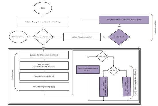
Figure 1.
A flowchart illustrating the process of the proposed mHGS optimizer.
3.2. The Satisfaction Fulfillment Step
This satisfaction fulfillment process is applied to the worst solutions whose probability of hungry weight is greater than 0.5.
where represents the new ith solution, is the current ith solution, and is a uniform number generated randomly through the range [0, 1].
3.3. The Binary τ-Based Crossover (τBX)
The crossover’s main objective is to enrich the children’s solutions with valuable information from the candidate parent’s solutions. Consequently, the generated children inherit the shared information from the parent’s characteristics. This helps a new solution to be generated by exchanging the information between the current solutions and the better parents’ solutions to inherent and generate promising offspring.
In binary crossover, two parents are selected for crossover and offspring, which are generated based on the similarity vector of the parents. This type of crossover simulates the binary crossover observed in nature such as the simulated binary crossover (SBC). In this study, a novel crossover mechanism is proposed called the binary τ-Based Crossover (τBX). This is explained mathematically as follows:
where is the crossover control parameter, explained as follows:
where is a vector of normally distributed random generators that is limited in the range of [0, 1], of the same size. The are the parent solutions, and are the two generated solutions after the crossover.
| Algorithm 1: Pseudo-code of the mHGS. |
| Input: 𝑁, 𝑀𝑎𝑥_FEs, 𝑙, 𝐷, 𝑆𝐻𝑢𝑛𝑔𝑟𝑦 parameters. |
| Output: Return 𝐵𝐹, 𝑋𝑏. |
| Initialization: Generate the initial positions of all solutions 𝑋𝑖 (𝑖 = 1,2, …, 𝑁). |
| While (FE ≤ 𝑀𝑎𝑥_FEs) |
| Compute the cost function values of all proposed solution |
| 𝑈𝑝𝑑𝑎𝑡𝑒 𝐵𝐹, 𝑊𝐹, 𝑋𝑏, 𝐵𝐼 |
| Compute the 𝐻𝑢𝑛𝑔𝑟𝑦 by Equation (8) |
| Compute the 𝑊1 by Equation (6) |
| For 𝑒𝑎𝑐𝒉 𝐼𝑛𝑑𝑖𝑣𝑖𝑑𝑢𝑎𝑙𝑠 |
| Update vb, VC1 in Equations (12) and (14). |
| 𝑈𝑝𝑑𝑎𝑡𝑒 𝑅 by Equation (4) |
| Apply the satisfaction fulfillment step in Equation (15) |
| End 𝐅𝐨𝐫 |
| 𝑡 = 𝑡 + 1 |
| End While |
| Return 𝐵𝐹, 𝑋𝑏 |
4. Experimental Series 1: Assessing mHGS in Solving Global Optimization Problems
The proposed mHGS efficiency was examined on the benchmark function test suite suggested in the IEEE-CEC’2020. Moreover, a comparative study was conducted between the simulation findings of the new mHGS and those resulting from several different classes of existing search algorithms, including the gravitational search algorithm (GSA) [31], whale optimization algorithm (WOA) [32], grey wolf optimizer (GWO) [33], Runge Kutta method (RUN) [34], and hunger search algorithm (HGS).
4.1. IEEE-CEC’2020 Test Suite
The IEEE-CEC’2020 test suite [35] was used to evaluate the performance of the proposed mHGS algorithms and the other competitors. Ten test functions, associated with the optimal values Fi*, were included in the CEC’2020 benchmark functions, including unimodal, multimodal, hybrid, and composition functions, as reported in Table 1. Moreover, the search range of [−100, 100]D was the same search range defined for all test functions.

Table 1.
CEC’2020 test suite description.
4.2. Parameters Setting
To establish a stable and fair assessment environment, the evaluation of the mHGS algorithm and the other comparative approaches was conducted for 30 experimental runs. Moreover, forty-five thousand function evaluations (FEs) were applied to all cases. Prior to conducting the searching process, some parameters were required to be initialized or set. The parameters of every algorithm, including the proposed mHGS, were defined according to Table 2. In engineering applications, identifying the appropriate set of parameter values that produces the optimal performance for every test method is a critical issue. Therefore, the Taguchi method for robust design parameters was applied. This method uses the Orthogonal Array (OA) and mean analysis to study the influence of these parameters’ variations on each algorithm according to the statistical measures of the experimental results. A fractional factorial matrix of numbers is structured in the OA so that each row denotes the level of factors in each run and each column denotes a particular variable that may be altered at each run.
Table 2.
Parameters’ values for the considered optimizers.
4.3. Statistical Analysis
To assess and compare the performances of the considered algorithms, a statistical analysis was conducted based on the outcomes of the CEC’2020 cost functions. This analysis includes the calculation of mean (AV) and standard deviation (SD) values of the resulting optimal solutions obtained at every experimental run. Table 3 shows the calculated mean and SD values obtained from each algorithm for the examined cost functions with a dimension of 10 parameters (Dim = 10). The boldface numbers in the table denote the best results.
Table 3.
The AV and SD of the 30-experimental-run study of the considered optimizers applied to the CEC’2020 cost functions when the dimension is 10.
The calculated average (AV) and its associated standard deviation SD values are illustrated in Table 3 for the 30-experimental-run study of the considered optimizers applied to the CEC’2020 benchmarks at Dim = 10. In the table, the resulting best (optimal) values are illustrated in boldface. As shown in Table 3, the new approach (mHGS) obtained the best result for the unimodal F1 cost function followed by the well-known GSA and RUN algorithms. Furthermore, the new mHGS performed well in the case of multi-modal F2, F3, and F4 cost functions. However, in the case of hybrid cost functions, F5, F6, and F7, the mHGS optimizer achieved a superior performance compared to the other competitor approaches. Alternatively, for the composite cost functions F8 to F10, the mHGS approach achieved a better result compared to the competitors, and was similar to the recent RUN on F10. Referring to the conducted Friedman test, the new mHGS performance was better than that of the GSA, WOA, GWO, RUN, and HGS. In a specific manner and based on the Friedman test, the mHGS was ranked first among all of the algorithms.
4.4. Converging Analysis
One of the essential analyses in the optimization field is convergence analysis. Therefore, the behaviors of the algorithms in reaching the best solutions were plotted, as shown in Figure 2. Each plot gives information about the speed and accuracy of its corresponding algorithm. By investigating the plots in Figure 2, the new mHGS optimizer shows a convergence curve that reaches the near-optimal solutions faster than most of the other algorithms. Accordingly, this proposed algorithm can be considered viable, especially for a problem that requires fast processing time such as the online-optimization applications.
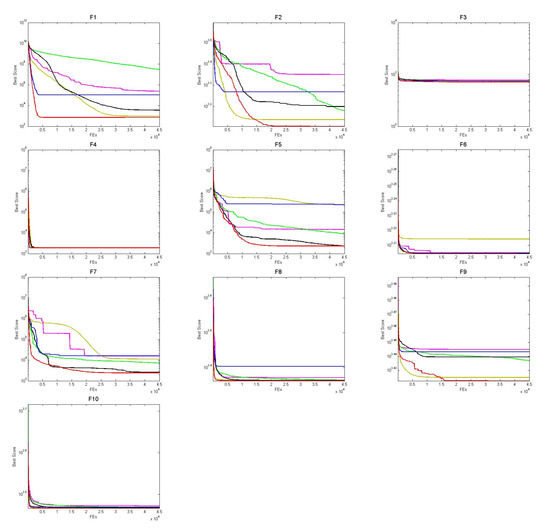
Figure 2.
Convergence plots of the new mHGS and the addressed optimizers for the CEC’2020 benchmarks where the dimension is 10.
4.5. Boxplot Behavior Analysis
The boxplot graph is a powerful tool that analyzes and explains graphically how the empirical data are distributed and where the data distributions are interpreted into quartiles [36]. The minimum and maximum edges of the boxplot whiskers refer to the highest and lowest obtained data values. Furthermore, the lower and upper ends of each rectangle represent both the lower and upper quartiles, respectively. Further, the boxplots illustrate the data distribution and its degree of agreement, noting that the narrower the boxplot the higher the symmetry between the obtained data. Figure 3 illustrates the distributed boxplots’ graphical representation of the results obtained for the ten CEC’20 cost functions, F1 to F10, when the problem’s dimension is 10. It demonstrates that, for most of the cost functions, the mHGS achieves narrower boxplot distributions that have minimum values relative to the other optimizers. Moreover, the plots in Figure 3 demonstrate that the new mHGS optimizer is consistent and is able to effectively locate the promising search areas.
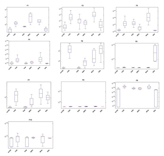
Figure 3.
The boxplot plots of the new mHGS and the addressed optimizers over the ten CEC’2020 benchmarks where the dimension is 10.
4.6. Wilcoxon Rank Test Analysis
Another test was conducted to exhibit the degree of significance for the resulting values, namely, the Wilcoxon rank-sum test. This test was applied to explore the difference between the new mHGS and the other competing optimizers. Details about the Wilcoxon test can be found in [37]. Despite MAs’ searching mechanism being naturally stochastic, their performances are still precise and acceptable in many applications. Accordingly, this test was used for the proposed mHGS algorithm outcomes, and proved that the algorithm’s findings are not only stable but also not stochastic. Table 4 presents the results of the Wilcoxon rank-sum test for the new mHGS and its five competitors, one by one, when applied to the ten cost functions, F1-F10. The criterion of comparison is based on the average value. The “Better”, “Similar”, and “Worse” labels denote the three expected cases of comparison when the mHGS is better, similar, or worse than the other method, respectively. To rely on the results shown in Table 4, they must be significant. Therefore, the significance test, known as “p-value”, is applied to decide whether the null hypothesis should be rejected or not. Basically, the significance value should be less than 5% to reject the null hypothesis. From the table, all the p-values (see the last column in Table 4) are less than 5%, which implies that the resulting values of Wilcoxon’s rank-sum test are reliable and significant.
Table 4.
The comparison and p-value results based on the Wilcoxon test for the ten CEC’2020 cost functions.
5. Experimental Series 2: Applying mHGS to Allocate Biomass Distributed Generators
5.1. Problem Formulation
If Pj and Qj represent the active and reactive power needed by the load, respectively, the power loss in this transmission line is defined by the following relation [25]:
Therefore, in the case of a distribution network, the total active power loss is expressed as follows [26]:
where denotes the bus number, the active and reactive demands at the nth bus are denoted by and , respectively, and is the voltage at the mth bus.
Equation (20) generalizes the active power loss expressed in Equation (19) using the following relation [26]:
where the number of generators is represented by , the generated power from the ith unit is represented by , and the output power from the jth unit is represented by .
The mathematical representation for the objective function is as follows [26]:
where the vector of generating-units’ power is denoted by , and the loss coefficients’ matrices are denoted by , , and .
5.2. Results and Discussion
The suggested strategy was applied to three different RDNs, IEEE 33-bus, IEEE 69-bus, and IEEE 119-bus. The suggested mHGS was performed with a 25-particle population size, a 2500-iteration optimization process, and 10 independent runs. Additionally, the results were compared with GSA, WOA, GWO, RUN, and original the HGS, in addition to the stochastic fractal search algorithm (SFSA) [38]. Moreover, Friedman and ANOVA statistical tests were used to prove the superiority of the suggested mHGS.
5.2.1. Objective: IEEE 33-Bus Network
The IEEE 33-bus comprises 33 nodes and 32 branches, and the nominal voltage and base MVA of the network are 12.66 kV and 100 MVA, respectively. The architecture of this network is shown in Figure 4. The active and reactive demands are 3.715 MW and 2.3 MVAr, respectively. The system data are validated in [36] and the active and reactive losses are found to be 210.99 kW and 143.13 kVAr, respectively. The considered cost function, which mitigates the total active power loss, is achieved via integrating the three biomass-based DGs into the network. The new mHGS is utilized to optimize the IEEE 33-bus compared to other optimizers, and the optimal obtained results are given in Table 5. The proposed mHGS succeeded in achieving the best power loss at a value of 11.6300 kW by installing three BDGs with sizes of 747.608, 1050.82, and 1081.29 kW with optimal power factors of 0.907, 0.718, and 0.901 on buses 14, 30, and 24, respectively. This integration mitigated the voltage deviation to 0.0006 pu. The voltage stability index (VSI) and its inverse (VSI−1) in this case were 0.9668 and 1.0343 pu, respectively. These results reveal that the network with the installed BDGs via the proposed mHGS is stable. By comparison, the conventional HGS achieved active power loss of 22.1601 kW via installing 847.683, 778.009, and 967.489 kW BDGs with 0.985, 0.605, and 0.735 power factors on buses 13, 32, and 24 respectively. Moreover, SFSA [38] achieved a power loss of 11.762 kW, mitigating it by 36.38%, via installing BDGs with active power of 792.7, 1030.0, and 1042.2 kW and reactive power of 374.7, 523.2, and 1015.2 kVAr on buses 13, 14, and 30 respectively. The worst power loss was 37.7552 kW, obtained via GSA. Regarding the loss reduction, the proposed mHGS achieved the best mitigation of 94.49%, whereas the worst one was HGS with 82.11%. The statistical parameters of best, worst, mean, median, variance, and SD for all considered optimizers were calculated and are tabulated in Table 6. The results reveal that the new optimizer is superior to the competitors in terms of best, worst, mean, and median, whereas for variance and Stand. Dev. it was not ranked first. However, the most important issue is that it achieved the best fitness value. Additionally, the computation time for one run was executed and is tabulated in Table 6; it is clear that the HGS and mHGS achieved the lowest computational times of 121.582 and 125.232 s, respectively.
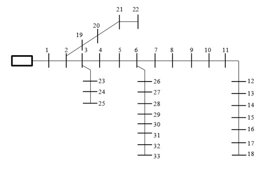
Figure 4.
IEEE 33-bus network layout.
Table 5.
The optimal results obtained via different optimizers applied to the IEEE 33-bus.
Table 6.
Statistical parameters of different optimizers applied to the IEEE 33-bus.
Figure 5 shows the voltage profile obtained through all the considered optimizers for the IEEE 33-bus network with and without BDGs. It is clear that the suggested mHGS helped in enhancing the network’s voltage profile compared to the other approaches. The variations in the fitness value throughout the optimization processes resulting from the considered approaches are illustrated in Figure 6. The curves confirm the superiority of the proposed mHGS in achieving the best performance compared to the others. The suggested mHGS confirmed its competence and superiority in integrating the BDGs into the IEEE 33-bus network.
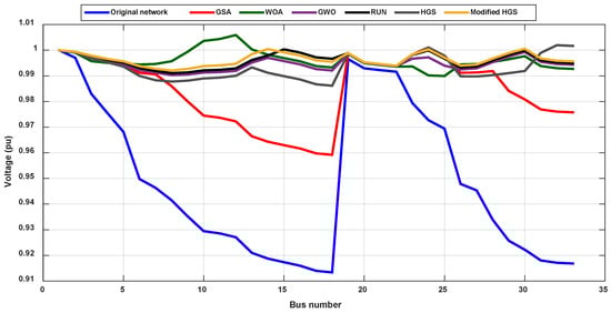
Figure 5.
IEEE 33-bus network voltage profiles with and without BDGs.
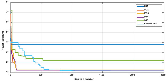
Figure 6.
Variation in power loss with iteration numbers of different optimizers applied to the IEEE 33-bus.
5.2.2. Objective: IEEE 69-Bus Network
The analysis was extended to the IEEE 69-bus network, which includes the 69-node and 68-branch configuration, as given in Figure 7. In this network, the nominal voltage and the MVA are 12.66 kV and 100 MVA, respectively. The total demands are 3.8 MW and 2.69 MVAr, while the total active and reactive power losses of the original network are 225 kW and 102.16 kVAr, respectively. Moreover, the voltage deviation of the original network is 0.099337 pu. The proposed mHGS, with the other algorithms, was applied to install three BDGs for mitigating the network active power loss, and the resulting values are listed in Table 7. The suggested mHGS outperformed the other considered approaches employed to install BDGs in the IEEE 69-bus network, achieving the best fitness value of 5.2291 kW with a loss reduction of 97.68%. To accomplish this goal, three BDGs have to be installed on buses 11, 18, and 61 in the network with the following features: capacities of 588.69, 369.57, and 1499.8 kW and power factors of 0.873, 0.819, and 0.78, respectively. In this case, the voltage deviation, VSI, and its inverse are 0.0005, 0.9670, and 1.0341 pu, respectively. Based on these results, and after installing the BDGs, the stability of the network was satisfied via the suggested approach. However, the conventional HGS achieved a power-loss value of 8.9086 kW with a reduction of 96.04%, which is less than the value obtained by the proposed algorithm. The worst case was obtained by the GSA optimizer, as it achieved a power loss of 22.6155 kW with only a reduction of 89.95% via installing 508.37, 499.89, and 1233.1 kW BDGs with 0.754, 0.299, and 0.844 power factors on buses 23, 8, and 61, respectively. Figure 8 illustrates the resulting voltage profiles via all considered optimizers of the considered IEEE 69-bus network with and without installing the BDGs. The curves show a great improvement in the network after installing the BDGs using the new approach. Moreover, Figure 9 shows the convergence curves of the fitness function for all considered algorithms applied to the investigated network. From the plotted curves, the superiority and competence can clearly be inferred for the suggested mHGS performance compared to the others.
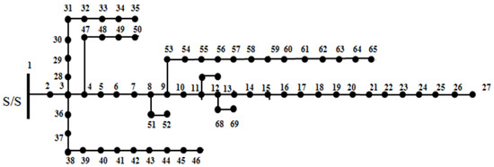
Figure 7.
IEEE 69-bus network configuration.
Table 7.
The resulting optimal values through different optimizers applied to the IEEE 69-bus.
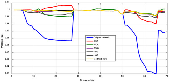
Figure 8.
IEEE 69-bus network voltage profiles with and without BDGs.
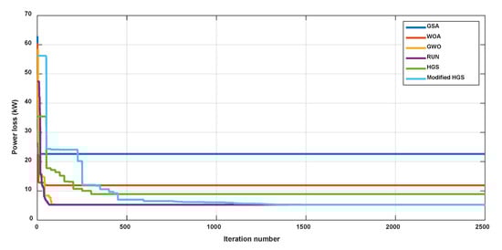
Figure 9.
Variation in power loss with iteration numbers of different optimizers applied to the IEEE 69-bus.
5.2.3. IEEE 119-Bus Network
Validating the new mHGS on a large-scale distribution network is essential to assess its capability. This can be performed via conducting the analysis on the IEEE 119-bus network as an example. The topology of a such network is given in Figure 10. This network contains 119-node and 115-tie-line architecture with a rated voltage and a base MVA of 11 kV and 100 MVA, respectively. The details of the network, including the branch and bus data, can be found in [39]. Moreover, the network’s active and reactive load power values are 22.709.7 kW and 17.041.1 kVAr, respectively. Furthermore, the overall active and reactive power losses of the original network are 1298.091 kW and 978.736 kVAr, respectively. The network has a voltage stability index of 0.5697 pu and a voltage deviation of 0.357641 pu. In this network, it is assumed that the five BDGs with maximum limits of 5 MW are integrated. The suggested approach was applied to the IEEE 1119-bus network, and the obtained results are tabulated in Table 8 in comparison with the other considered approaches. The new mHGS suggested installing five BDGs with capacities of 1554.5, 1544.9, 3302.2, 2641.2, and 3209.0 kW with power factors of 0.748, 0.874, 0.757, 0.879, and 0.698 on buses 43, 94, 114, 75, and 81, respectively. This integration reduced the network’s active power loss to 145.489 kW with a power reduction of 88.79%. Moreover, the voltage deviation, VSI, and its inverse in this case were 0.0159, 0.8753, and 1.1425 pu, respectively. The results reveal that the network is stable after installing the BDGs based on locations and sizes obtained via the proposed mHGS. The RUN algorithm was ranked second, with an active power loss of 152.6763 kW and a reduction of 88.24%. The worst approach was GSA, which achieved power loss of 665.4651 kW. Figure 11 shows the voltage profiles of the network with and without installing the BDGs through all the considered optimizers. Figure 12 shows the convergence curves of the fitness function for all considered algorithms applied to the investigated network. From the plotted curves, the superiority and competence can also be inferred for the suggested mHGS performance compared to the others.
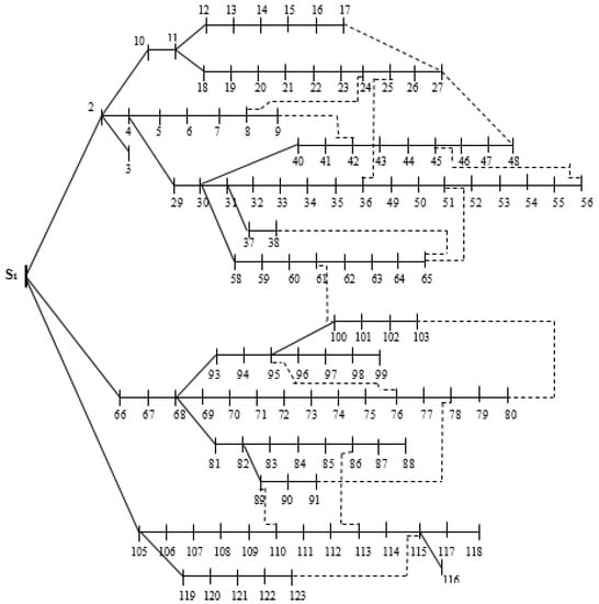
Figure 10.
IEEE 119-bus network configuration.
Table 8.
The optimal results obtained via different optimizers applied to the IEEE 119-bus.
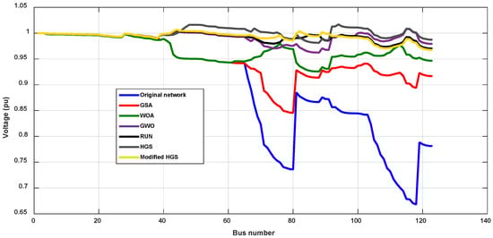
Figure 11.
IEEE 119-bus network voltage profiles with and without BDGs.
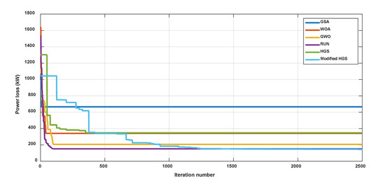
Figure 12.
Convergence curves of power loss against iteration numbers of different optimizers applied to the IEEE 119-bus.
Based on the obtained results mentioned above, it can be concluded that the new mHGS approach is competent and reliable when installing the biomass-based DGs in the radial distribution network. This was confirmed by applying the suggested approach to three different networks.
6. Conclusions
This paper presents a new modified variant of hunger games search (HGS) called mHGS for solving global optimization and biomass distributed generator (BDG) problems. The proposed mHGS approach includes a new binary τ-Based Crossover (τBX) strategy with the satisfaction fulfillment step mechanisms. This strategy proposed solutions to overcome the drawbacks of the classical hunger games search in dealing with global optimization problems, such as the BDG problems. The new mHGS performance was evaluated through ten IEEE CEC’2020 benchmarks against five competitive algorithms. The results of the proposed mHGS were compared to the findings of the other optimizers based on the statistical values of the Wilcoxon sign rank and Friedman tests. Then, the best distribution of the BDGs in a radial distribution network (RDN) was determined by mHGS to enhance the stabilization of the network. Three distribution networks of IEEE 33-bus, IEEE 69-bus, and IEEE 119-bus were considered to validate the superiority of the proposed mHGS. The resulting performance was compared with those resulting from the GSA, WOA, GWO, RUN, and original HGS optimizers. The new mHGS is capable of reducing the power loss to 11.6300, 5.2291, and 145.489 kW, with loss reduction of 94.49%, 97.68%, and 88.79% for the IEEE 33-bus, 69-bus, and 119-bus networks, respectively. These results showed that the new approach outperformed the other considered approaches. Therefore, the success of using other sources of energy, such as biomass-based fuel, will definitely help in reducing the massive use of CO2-based fuels, and hence reduce the CO2 emissions. A multi-objective version of mHGS is recommended in future work to mitigate both power loss and voltage deviation of distribution networks.
Author Contributions
Conceptualization, A.M.N. and A.F.; methodology, E.H.H. and H.R.; software, E.H.H. and H.R.; validation, A.M.N. and A.F.; formal analysis, E.H.H. and H.R.; investigation, E.H.H. and H.R.; resources, A.M.N. and A.F.; data curation, A.M.N. and A.F.; writing—original draft preparation, A.M.N., E.H.H., H.R. and A.F.; writing—review and editing, A.M.N., E.H.H., H.R. and A.F.; visualization, E.H.H. and H.R.; funding acquisition, A.M.N. All authors have read and agreed to the published version of the manuscript.
Funding
The authors extend their appreciation to the Deputyship for Research & Innovation, Ministry of Education in Saudi Arabia for funding this research work through the project number (IF2/PSAU/2022/01/22030).
Institutional Review Board Statement
Not applicable.
Informed Consent Statement
Not applicable.
Data Availability Statement
Not applicable.
Conflicts of Interest
The authors declare no conflict of interest.
Nomenclature
| Number in the range of [−𝑎, 𝑎] | A and B | Two positions selected randomly over the population size | |
| , and | Normally distributed random generators | Hungry weight of each solution | |
| 𝑡 | Index of the current step | Current function evaluation number | |
| and | Weight values of hunger | Maximum number of function evaluations | |
| Location of the best solution in the current step | New ith solution | ||
| Current solution’s position | Current ith solution | ||
| Constant parameter | Crossover control parameter | ||
| Objective function value of the ith solution | Vector of random numbers range [0, 1] | ||
| Best objective value in the current step | Parent solutions | ||
| Random number in range [0, 1] | Two generated solutions after the crossover | ||
| Uppermost number of function evaluations | Pj and Qj | Active and reactive demand powers at jth bus | |
| Hunger feeling of the solution | Buses number | ||
| The proposed number of solutions | Voltage at the mth bus | ||
| Sum of hungry features of all current solutions | Number of generators | ||
| , , and | Random numbers in the range [0, 1] | Vector of generating units’ powers | |
| WF | Current worst objective value | , , and | Loss coefficients’ matrices |
| and | Lower are the upper boundaries of the considered parameters | New ith solution | |
| and | Two solutions generated by the crossover strategy |
References
- Wilberforce, T.; Olabi, A.G.; Sayed, E.T.; Elsaid, K.; Abdelkareem, M.A. Progress in carbon capture technologies. Sci. Total Environ. 2021, 761, 143203. [Google Scholar] [CrossRef] [PubMed]
- Herbert, G.J.; Krishnan, A.U. Quantifying environmental performance of biomass energy. Renew. Sustain. Energy Rev. 2016, 59, 292–308. [Google Scholar] [CrossRef]
- Korberg, A.D.; Mathiesen, B.V.; Clausen, L.R.; Skov, I.R. The role of biomass gasification in low-carbon energy and transport systems. Smart Energy 2021, 1, 100006. [Google Scholar] [CrossRef]
- Sun, Z.; Liu, H.; Bai, H.; Yu, S.; Russell, C.K.; Zeng, L.; Sun, Z. The crucial role of deoxygenation in syngas refinement and carbon dioxide utilization during chemical looping-based biomass gasification. Chem. Eng. J. 2022, 428, 132068. [Google Scholar] [CrossRef]
- Habibollahzade, A.; Ahmadi, P.; Rosen, M.A. Biomass gasification using various gasification agents: Optimum feedstock selection, detailed numerical analyses and tri-objective grey wolf optimization. J. Clean. Prod. 2021, 284, 124718. [Google Scholar] [CrossRef]
- Díaz González, C.A.; Pacheco Sandoval, L. Sustainability aspects of biomass gasification systems for small power generation. Renew. Sustain. Energy Rev. 2020, 134, 110180. [Google Scholar] [CrossRef]
- Caglar, B.; Tavsanci, D.; Biyik, E. Multiparameter-based product, energy and exergy optimizations for biomass gasification. Fuel 2021, 303, 121208. [Google Scholar] [CrossRef]
- Pandey, B.; Sheth, P.N.; Prajapati, Y.K. Air-CO2 and oxygen-enriched air-CO2 biomass gasification in an autothermal downdraft gasifier: Experimental studies. Energy Convers. Manag. 2022, 270, 116216. [Google Scholar] [CrossRef]
- Houssein, E.H.; Mahdy, M.A.; Shebl, D.; Mohamed, W.M. A Survey of Metaheuristic Algorithms for Solving Optimization Problems. In Metaheuristics in Machine Learning: Theory and Applications; Springer: Cham, Germany, 2021; pp. 515–543. [Google Scholar]
- Houssein, E.H.; Mahdy, M.A.; Blondin, M.J.; Shebl, D.; Mohamed, W.M. Hybrid slime mould algorithm with adaptive guided differential evolution algorithm for combinatorial and global optimization problems. Expert Syst. Appl. 2021, 174, 114689. [Google Scholar] [CrossRef]
- Houssein, E.H.; Mahdy, M.A.; Eldin, M.G.; Shebl, D.; Mohamed, W.M.; Abdel-Aty, M. Optimizing quantum cloning circuit parameters based on adaptive guided differential evolution algorithm. J. Adv. Res. 2021, 29, 147–157. [Google Scholar] [CrossRef]
- Izci, D.; Ekinci, S. A novel improved version of hunger games search algorithm for function optimization and efficient controller design of buck converter system. E-Prime-Adv. Electr. Eng. Electron. Energy 2022, 2, 100039. [Google Scholar]
- Chakraborty, S.; Saha, A.K.; Chakraborty, R.; Saha, M.; Nama, S. HSWOA: An ensemble of hunger games search and whale optimization algorithm for global optimization. Int. J. Intell. Syst. 2022, 37, 52–104. [Google Scholar] [CrossRef]
- Ma, B.J.; Liu, S.; Heidari, A.A. Multi-strategy ensemble binary hunger games search for feature selection. Knowl. -Based Syst. 2022, 248, 108787. [Google Scholar] [CrossRef]
- Li, S.; Li, X.; Chen, H.; Zhao, Y.; Dong, J. A Novel Hybrid Hunger Games Search Algorithm With Differential Evolution for Improving the Behaviors of Non-Cooperative Animals. IEEE Access 2021, 9, 164188–164205. [Google Scholar] [CrossRef]
- AbuShanab, W.S.; Abd Elaziz, M.; Ghandourah, E.I.; Moustafa, E.B.; Elsheikh, A.H. A new fine-tuned random vector functional link model using Hunger games search optimizer for modeling friction stir welding process of polymeric materials. J. Mater. Res. Technol. 2021, 14, 1482–1493. [Google Scholar] [CrossRef]
- Abo El-Ela, A.A.; Allam, S.M.; Shaheen, A.M.; Nagem, N.A. Optimal allocation of biomass distributed generation in distribution systems using equilibrium algorithm. Int. Trans. Electr. Energy Syst. 2021, 31, e12727. [Google Scholar] [CrossRef]
- Barik, S.; Das, D. A novel Q−PQV bus pair method of biomass DGs placement in distribution networks to maintain the voltage of remotely located buses. Energy 2020, 194, 116880. [Google Scholar] [CrossRef]
- Ajeigbe, O.A.; Munda, J.L.; Hamam, Y. Optimal allocation of renewable energy hybrid distributed generations for small-signal stability enhancement. Energies 2019, 12, 4777. [Google Scholar] [CrossRef]
- Tanwar, S.S.; Khatod, D.K. Techno-economic and environmental approach for optimal placement and sizing of renewable DGs in distribution system. Energy 2017, 127, 52–67. [Google Scholar] [CrossRef]
- Das, B.; Mukherjee, V.; Das, D. Optimum placement of biomass DG considering hourly load demand. Energy Clim. Chang. 2020, 1, 100004. [Google Scholar] [CrossRef]
- Gómez-González, M.; Ruiz-Rodriguez, F.J.; Jurado, F. Metaheuristic and probabilistic techniques for optimal allocation and size of biomass distributed generation in unbalanced radial systems. IET Renew. Power Gener. 2015, 9, 653–659. [Google Scholar] [CrossRef]
- Gomez-Gonzalez, M.; Ruiz-Rodriguez, F.J.; Jurado, F. Probabilistic optimal allocation of biomass fueled gas engine in unbalanced radial systems with metaheuristic techniques. Electr. Power Syst. Res. 2014, 108, 35–42. [Google Scholar] [CrossRef]
- Zou, K.; Agalgaonkar, A.P.; Muttaqi, K.M.; Perera, S. Distribution system planning with incorporating DG reactive capability and system uncertainties. IEEE Trans. Sustain. Energy 2011, 3, 112–123. [Google Scholar] [CrossRef]
- Fathy, A. A novel artificial hummingbird algorithm for integrating renewable based biomass distributed generators in radial distribution systems. Appl. Energy 2022, 323, 119605. [Google Scholar] [CrossRef]
- Fathy, A.; Yousri, D.; Rezk, H.; Ramadan, H.S. An efficient capuchin search algorithm for allocating the renewable based biomass distributed generators in radial distribution network. Sustain. Energy Technol. Assess. 2022, 53, 102559. [Google Scholar] [CrossRef]
- Balu, K.; Mukherjee, V. Optimal allocation of electric vehicle charging stations and renewable distributed generation with battery energy storage in radial distribution system considering time sequence characteristics of generation and load demand. J. Energy Storage 2023, 59, 106533. [Google Scholar] [CrossRef]
- Raut, U.; Mishra, S. An improved equilibrium optimiser-based algorithm for dynamic network reconfiguration and renewable DG allocation under time-varying load and generation. Int. J. Ambient. Energy 2022, 1–25. [Google Scholar] [CrossRef]
- Khasanov, M.; Kamel, S.; Halim Houssein, E.; Rahmann, C.; Hashim, F.A. Optimal allocation strategy of photovoltaic-and wind turbine-based distributed generation units in radial distribution networks considering uncertainty. Neural Comput. Appl. 2022, 1–26. [Google Scholar] [CrossRef]
- Yang, Y.; Chen, H.; Heidari, A.A.; Gandomi, A.H. Hunger games search: Visions, conception, implementation, deep analysis, perspectives, and towards performance shifts. Expert Syst. Appl. 2021, 177, 114864. [Google Scholar] [CrossRef]
- Rashedi, E.; Nezamabadi-Pour, H.; Saryazdi, S. GSA: A gravitational search algorithm. Inf. Sci. 2009, 179, 2232–2248. [Google Scholar] [CrossRef]
- Mirjalili, S.; Lewis, A. The whale optimization algorithm. Adv. Eng. Softw. 2016, 95, 51–67. [Google Scholar] [CrossRef]
- Mirjalili, S.; Mirjalili, S.M.; Lewis, A. Grey wolf optimizer. Adv. Eng. Softw. 2014, 69, 46–61. [Google Scholar] [CrossRef]
- Ahmadianfar, I.; Heidari, A.A.; Gandomi, A.H.; Chu, X.; Chen, H. RUN beyond the metaphor: An efficient optimization algorithm based on Runge Kutta method. Expert Syst. Appl. 2021, 181, 115079. [Google Scholar] [CrossRef]
- Houssein, E.H.; Rezk, H.; Fathy, A.; Mahdy, M.A.; Nassef, A.M. A modified adaptive guided differential evolution algorithm applied to engineering applications. Eng. Appl. Artif. Intell. 2022, 113, 104920. [Google Scholar] [CrossRef]
- Williamson, D.F.; Parker, R.A.; Kendrick, J.S. The box plot: A simple visual method to interpret data. Ann. Intern. Med. 1989, 110, 916–921. [Google Scholar] [CrossRef]
- Wilcoxon, F. Individual comparisons by ranking methods. In Breakthroughs in Statistics; Springer: New York, NY, USA, 1992; pp. 196–202. [Google Scholar]
- Raut, U.; Mishra, S. A new Pareto multi-objective sine cosine algorithm for performance enhancement of radial distribution network by optimal allocation of distributed generators. Evol. Intell. 2021, 14, 1635–1656. [Google Scholar] [CrossRef]
- Zhang, D.; Fu, Z.; Zhang, L. An improved TS algorithm for loss-minimum reconfiguration in large-scale distribution systems. Electr. Power Syst. Res. 2007, 77, 685–694. [Google Scholar] [CrossRef]
Disclaimer/Publisher’s Note: The statements, opinions and data contained in all publications are solely those of the individual author(s) and contributor(s) and not of MDPI and/or the editor(s). MDPI and/or the editor(s) disclaim responsibility for any injury to people or property resulting from any ideas, methods, instructions or products referred to in the content. |
© 2023 by the authors. Licensee MDPI, Basel, Switzerland. This article is an open access article distributed under the terms and conditions of the Creative Commons Attribution (CC BY) license (https://creativecommons.org/licenses/by/4.0/).