Abstract
A computational fluid dynamic (CFD) simulation is performed to evaluate the resistance performance of a self-propelled amphibious vessel with caterpillars to be operated as a marine debris collection vessel at hard-to-reach areas. This study focuses on the influence of the addition of caterpillars on the vessel to the resistance performance. To capture the free surface model, the volume of fluid (VOF) method was adopted, and to express the sinkage and trim acting on the ship the Dynamic Fluid-body Interaction (DFBI) model was applied. A series of numerical simulations for resistance performance were carried out in the range of Froude number (Fn) of 0.12–0.32 for the vessels with and without caterpillars. A model test was carried out independently to verify the numerical simulation of resistance, and it indicated that the present simulation is valid with relative errors of less than 2% over the entire speed range. In subsequence, the resistance performance of the ship due to the addition of the caterpillars was evaluated, and an increase of nearly 40% at the design speed of Fn = 0.27 could be observed. In addition, in the present amphibious vessel, it was found that the ratio of the pressure resistance occupied in the total resistance was dominant, reaching around 81~92% for both cases.
1. Introduction
An amphibious vehicle is specially designed to be operated both on land and in the water. The first known self-propelled amphibious vehicle was invented by Oliver Evans [1]. In World War II, amphibious vehicles were used to carry and transport armor [2]. However, amphibious vehicles were then widely developed into multipurpose vehicles such as amphibious bicycles, cars, buses, etc., that were usually used to transport passengers or means. Recently, unmanned or autonomous amphibious vehicles are widely used.
In the present study, a twin-hull self-propelled amphibious vehicle was developed to collect marine debris at hard-to-reach areas, whereas usually these kinds of vessels are designed for military use. This vessel was designed with caterpillars on both hulls. A caterpillar amphibious vehicle was invented in 1987 in China by Liu Shi Yuan [3] and is currently being developed by Lee and Lee [4] to stably receive the driving force without slipping from the driving sprockets. In the past invention, a caterpillar amphibious vehicle was applicable for farming and transportation vehicles, and since it can amphibiously travel, could also be used for water transportation. This caterpillar is suitable to use without destroying the road surface and has a walking structure that is applicable to the amphibious vehicles. The addition of caterpillars on the ship affects the resistance because the caterpillar is considered an appendage of the ship. Installing appendages to a ship is a simple way to improve some of the performance of the ship, but on the other hand, it can also give some other disadvantages. In other words, in the case of the caterpillar equipped on the vessel, it helps the movement without significantly adding air resistance when moving on land, but it increases the resistance in the water.
Some studies of amphibious vehicle resistance have been performed, such as in the study proposed by Pan et al. [5]. Nakisa et al. [6] performed a Reynolds-averaged Navier–Stokes (RaNS) simulation of viscous flow around the hull of a multipurpose amphibious vehicle. Jaouad et al. [7] also proposed a study of computational fluid dynamic (CFD) analysis of an amphibious vehicle. The study focused on minimizing drag and improving the aerodynamic performance characteristic of an amphibious vehicle. Yamshita et al. [8] presented a methodology for the simulation of amphibious craft transitioning between land and marine modes in the surf zone. Another study of the improvement of resistance performance of amphibious vehicles was proposed by Sun et al. [9]. A study of an investigation of the addition of stern flaps on an amphibious vehicle was conducted to improve the resistance performance. Meanwhile, Jang et al. [10] proposed a study of the hydrodynamics performance of a different kind of amphibious vehicle, the Wheeled Armored Vehicle (WAV). Recently, Du et al. [11] made an investigation of critical parameters influencing the resistance performance of an amphibious vehicle.
However, a study of the influence of caterpillars on the resistance performance of an amphibious vehicle has never been conducted before. Therefore, in this study, a numerical resistance simulation is conducted to evaluate the added resistance due to the influence of caterpillars on the amphibious vehicle.
2. Numerical Simulation
The numerical simulation with CFD method was performed to evaluate the resistance performance of an amphibious vehicle both with and without caterpillars using a commercial software, Star CCM+ ver16.04.007.
2.1. Governing Equations
The numerical analysis was performed by the RaNS simulation with the continuity and momentum conservation equations as follows:
where is the cartesian component of the total velocity vector, is the position, is the time, is the density, is the pressure, is the kinematic viscosity, is the gravitational acceleration, and is the Reynolds stress or turbulent stress term.
In this study, the SST turbulence model was used to model the Reynolds stress term for numerical simulation, considering this model gives the most accurate result compared with other turbulence models. The simulation with the realizable turbulence model was also antecendently evaluated, and the validation with the experiment gave up to 15% error range for the realizable turbulence model and less than 2% for the SST turbulence model. Therefore, the realizable turbulence model was selected to the subsequent simulation. The equations of the SST turbulence model can be written as:
where and indicate the turbulence kinetic energy and the specific rate of dissipation, respectively and and represent the active diffusivity of and . and express the turbulence kinetic energy due to mean velocity gradients and . and express the dissipation of and due to turbulence. Additionally, expresses the cross-diffusion term. Meanwhile, and are user-defined source terms [12].
For capturing the free-surface movement, the volume-of-fluid (VOF) model was adopted. The VOF model tracks the volume fraction instead of the free-surfaces height. This model was developed from studies of two-phase (water and steam) problems and the concept of volume fraction was first extended to discontinuous variables to locate the free-surface in an incompressible fluid by Nichols and Hirt [13]. Assuming the free-surface as a funtion of space and time, its value will range between zero (air) and one (water) [14]. Initially, is set to zero and one in the air and water domains, respectively, indicating a nearly discontinuous distribution with respect to the free-surface. However, while the calculation is in progress, the transport Equation (5) for F is solved so that all calculation cells have a continuous scalar value of . Among them, the iso-surface with is defined as a free surface.
Since the discretization of Equation (5) is accompanied by temporal and spatial numerical instability and/or diffusion depending on the numerical scheme used, various techniques such as introducing a source term on the right side have been proposed to control. The detailed numerical treatments in STAR-CCM+ used in this study are given in [15].
2.2. Computational Configuration
An implicit unsteady simulation with a time step of 0.01 s and an asymptotic stopping criterion as a convergence parameter was set in this simulation. An SST (Shear Stress Transport) as the turbulence model was employed and the resistance simulation was conducted under a running trim condition. To express the sinkage and trim acting on the ship, the Dynamic Fluid-body Interaction (DFBI) Rotation and Translation model was applied, and Z motion and Y rotation were set as the representative of two degrees of freedom (2-DOF) of motion: heave and pitch.
2.2.1. Simulation Object
Two models are being evaluated in this study: a ship with and without caterpillars. The main dimensions of the ships are shown in Table 1 and the geometric models of the ships are shown in Figure 1. A ship with a length (LOA) of 10.767 m and model scale of 1:10.767 was used for the numerical simulation. The flow parameters of the scaled model were determined using the Froude number (Fn) as a scale factor, which considers the length (L) and speed (V) of the vessel based on the Froude similarity law.

Table 1.
Main dimensions of the vessels.
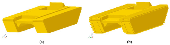
Figure 1.
Geometric model of the vessels; (a) w/o caterpillar, (b) w/caterpillar.
2.2.2. Mesh Generation and Boundary Conditions
Based on ITTC Practical Guidelines for ship resistance CFD [16], the simulation boundaries were set as 1.5 L from the inlet, side, and bottom; 2.5 L from the outlet; and 0.5 L from the top as shown in Figure 2. With velocity inlet for the inlet, bottom, top, and side, and pressure outlet for the outlet as boundary conditions, the simulations were performed. Then, the symmetry boundary was applied to treat only half of the model for the simulation. Meanwhile, the ship hull was treated as a nonslip wall.
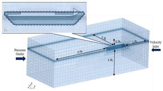
Figure 2.
Mesh configuration and computational domain.
As shown in Figure 2, a trimmed cell mesh as the core volume mesh with twelve prism layers on the ship hull and six prism layers on the caterpillar as the boundary layer mesh was applied for this simulation. To obtain the suitable configuration and number of grids, grid independence was performed, and the Grid Convergence Index (GCI) was calculated. The GCI was an indicator used for the determination of the grid by calculating the convergence error of the grid based on Richardson’s extrapolation [17]. Five different sizes of the grid were varied and through the GCI the grid configuration with the optimal grid number was used for further simulation. The results of the GCI calculation are shown in Table 2. Here, represents the refinement ratio and expresses the order of discretization error or the order of accuracy. expresses the total resistance (RT) at zero grid spacing. Meanwhile, and represent the GCI of the fine grid and course grid, respectively. Meanwhile, Figure 3 shows the plot of the total resistance and GCI to the grid refinement. Through the GCI calculation, it was found that the optimum grid had a size of 0.0177 m and the number of grids was about 2.56 M.
Table 2.
Grid convergence index (GCI).
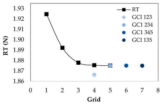
Figure 3.
Grid independence index (GCI).
3. Result and Discussion
Resistance simulation was evaluated in 10 variations of Fn for an amphibious vehicle with caterpillars and 12 variations of Fn for an amphibious vehicle without caterpillars. Meanwhile, the Fn for the actual service speed of the amphibious vehicle was 0.27.
3.1. Numerical Simulation Results
The results of the numerical resistance simulation for both ships with and without caterpillars are shown in Table 3 and Figure 4. Table 3 shows the results of the simulation of five representative results of total variation speeds. Since the ship’s resistance was directly proportional to the square of the ship’s speed, the total resistance increased significantly when the ship’s speed increased as shown in Figure 4. The addition of caterpillars on the vessel increased the ship’s resistance for all ship speed variations by an average of 39.2%. In the case of total resistance at the service speed, it increased up to 36.8% from the ship without caterpillars with a total resistance of 2.486 N to 3.937 N. As expected, the addition of caterpillars on the vessel gave a significant effect to the ship’s resistance. Since the vessel will be operated in low-speed conditions it does not give a big impact on the ship’s power, so it still worthwhile and applicable.
Table 3.
Numerical simulation results of vessels w/and w/o caterpillars.
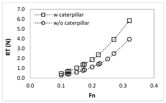
Figure 4.
Numerical simulation results of vessels w/and w/o caterpillars.
3.1.1. Components of Total Resistance
To further evaluate the influence of the caterpillars added to the vessel, two components of the total resistance of the vessel were classified: pressure resistance (RP) and friction resistance (RF). Then, they were represented by coefficients of resistance based on the wetted surface area (), total resistance coefficient (), friction coefficient (), and pressure coefficient () as indicated in Table 4 and Figure 5. Table 4 shows that the differences in friction resistance and pressure resistance between the ship with and without caterpillars are on average 22.6% and 43.0%, respectively. This implies that the addition of caterpillars increases the pressure resistance significantly more than that of the friction resistance. On the other hand, in the present amphibious vessel, it was found that the ratio of the pressure resistance occupied in the total resistance was dominant, reaching around 81~92% for both cases.
Table 4.
Components of resistance coefficient (Ct, Cf, and Cp).
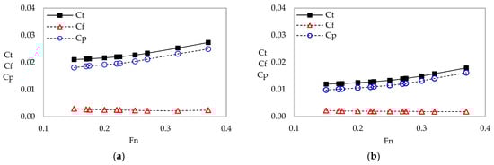
Figure 5.
Components of resistance coefficient (Ct, Cf, and Cp): (a) w/ caterpillars, (b) w/o caterpillars.
3.1.2. Trim and Sinkage
The results of trim and sinkage of the amphibious vehicle with and without caterpillars are shown in Figure 6 and Figure 7, respectively. For both cases, the trim and sinkage of the vessel with caterpillars were higher than that of the vessel without caterpillars. The higher Fn showed a significant increasing in trim for the vessel with caterpillars. However, the trim was very small, with the average trim less than 0.1 degrees for both ships with and without caterpillars. Figure 6 shows that the trim value is less than zero, which indicates that the vessel was trimmed by stern.
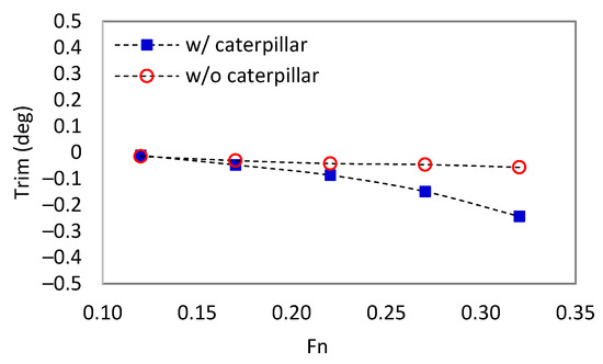
Figure 6.
Trim for the vessels w/and w/o caterpillars.
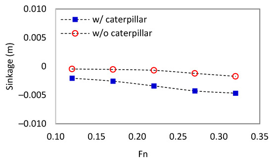
Figure 7.
Sinkage for the vessels w/and w/o caterpillars.
3.1.3. Pressure and Shear Stress Distribution
Not only the component of total resistance but also the distribution of pressure and shear stress of the ship hull were being investigated. As shown in Figure 8, the pressure distribution around the ship’s hull with caterpillars (above) was higher than that of the ship without caterpillars (below). A high-pressure distribution was indicated especially at the bottom part of the hull. That is why the increase of the pressure coefficient between the ship with and without caterpillars reached up to 43.0%, as explained before. Meanwhile, for the shear stress, there was an increase of shear stress or friction coefficient up to 22.6%, as explained before, and it was proved by the stress distribution as shown in Figure 8. The shear stress distribution at the bottom part of the caterpillar indicated that the shear stress of the ship with caterpillars was higher than that of the ship without caterpillars. The high shear stress distribution was also being captured at the front hull of the ship without caterpillars.
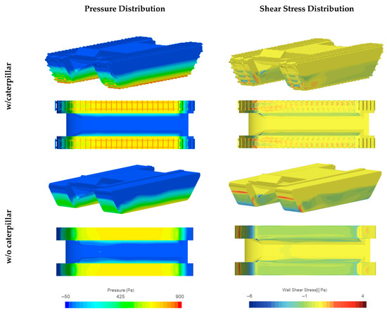
Figure 8.
Comparison of pressure and shear stress distribution at Fn = 0.27.
3.1.4. Wave Profile
Figure 9 shows the wave profiles along the hull of the vessel with caterpillars compared with the vessel without caterpillars at Fn = 0.27. Based on the plot, especially from the bow (x/L = 1) to the midship (x/L = 0.5), it seems that the wave profiles along the hull illustrate a large difference depending on the presence or absence of caterpillars, which can be explained by the existence of the complex-shaped caterpillars, which greatly contributed to the dramatic attenuation of the bow waves.
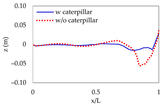
Figure 9.
Wave profiles along the hull of vessels w/and w/o caterpillars at Fn = 0.27.
3.1.5. Wave Configuration
Figure 10 shows the wave elevation of the ship with caterpillars at Fn of 0.17, 0.22, 0.27, and 0.32, respectively. Meanwhile, the wave elevation of the ship without caterpillars are captured in Figure 11. In general, the wave elevation became rougher with the increase of the ship’s speed. By investigating the wave elevation at the part of the divergent wave, there seemed to be no significant behavior between the ships with and without caterpillars. However, a significant wave elevation was captured at the front and behind the ships with and without caterpillars. The ship with caterpillars had a rougher wave at the front hull, but it was becoming calm behind the hull. On the other hand, for the ship without caterpillars, the wave was calm at the front hull and became rougher behind the hull. This indicates that the addition of the caterpillars interferes with the transverse wave of the ship.
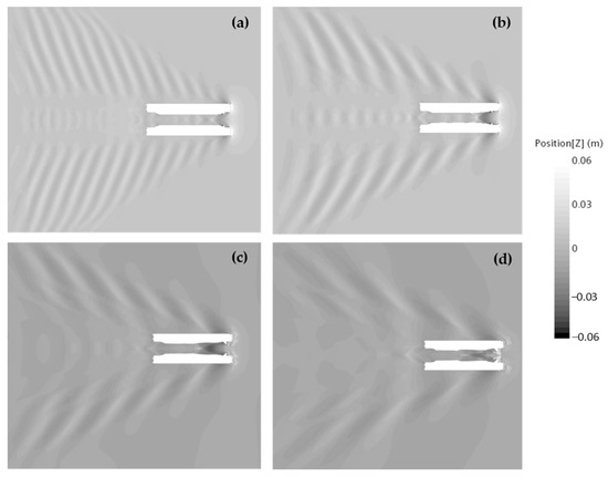
Figure 10.
Wave pattern of amphibious vehicle w/caterpillars at Fn of: (a) 0.17, (b) 0.22, (c) 0.27, (d) 0.32.

Figure 11.
Wave pattern of amphibious vehicle w/o caterpillars at Fn of: (a) 0.17, (b) 0.22, (c) 0.27, (d) 0.32.
3.2. Validation with Experiment
To validate the results of the CFD simulation, the model test was conducted in the towing tank of Changwon National University, Korea. As shown in Figure 12, the model was attached to the frame structure in the middle of the towing carriage. The resistance acting on the hull was measured by the load cell, which was installed on the model and its connection between model and frame structure. Figure 13 shows the relationship between the measuring force and the output voltage of the amplifier of the load cell. The calibration factor of the load cell was 1/43.662. The electrical signal received from the load cell was amplified by an amplifier. Additionally, then, the electrical signal of the output from the load cell was converted by the A/D converter into digital signals. The capacity of the load cell was 2 N. Therefore, a clamp system was used to avoid overloading the load cell. During acceleration and deceleration, the model was clamped to prevent it from becoming unstable and moving too much. The clamp was automatically released when the carriage achieved the target towing speed, and after the carriage stopped, the clamps closed again before returning to the starting position.
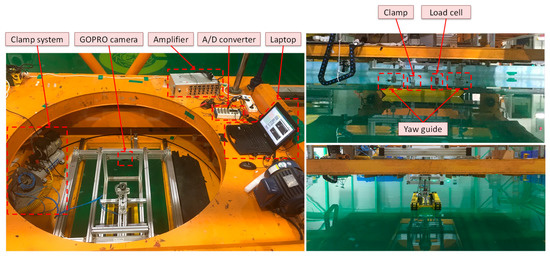
Figure 12.
Experimental setup for resistance test.
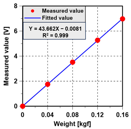
Figure 13.
Result of load cell’s calibration.
The model was towed at various ship speeds. However, because of the limit of the load cell calibration, the experiments were only capable to accommodate the model test up to Fn = 0.2 for the vessel with caterpillars and Fn = 0.25 for the vessel without caterpillars. The model test results are illustrated in Figure 14.
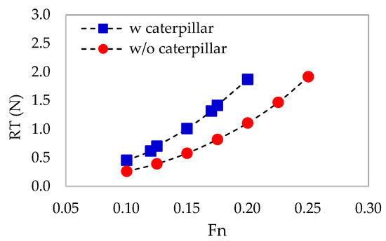
Figure 14.
Model test results of an amphibious vehicle w/and w/o caterpillars.
The comparison of the numerical simulation with the experimental result is shown in Table 5 and Figure 15. It shows that the difference between the numerical simulation results and the model test results was less than 2%. This indicates that the numerical simulation is valid and accepted. As explained before, because of the limit of towing tank facility, the model test could only be carried out up to Fn = 0.25. Therefore, the numerical simulation with Fn more than 0.25 could not be verified with this experiment. The problem was that the service speed of the ship was out of the range of speed that could be accommodated with the model test. So, a statistical measure of the regression model that represents the proportion of the variance for a dependent variable was calculated. As shown in Figure 16, the value of of the total resistance results for both ships with and without caterpillars were close to one, indicating a high level of correlation and considered a reliable value.
Table 5.
Validation of numerical simulation with experiment.
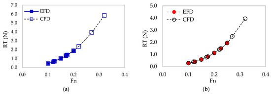
Figure 15.
Validation of CFD with experiments of amphibious vehicles; (a) w/caterpillars, (b) w/o caterpillars.
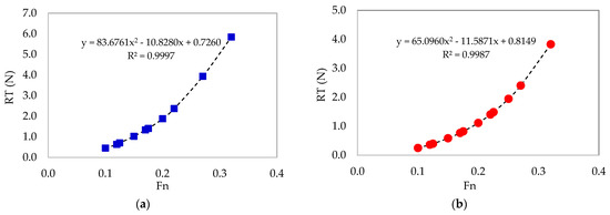
Figure 16.
Statistical measure for total resistance for amphibious vehicles: (a) w/caterpillars, (b) w/o caterpillars.
4. Conclusions
In this study, the influence of caterpillars to an amphibious vehicle on the resistance is analyzed through numerical simulation using CFD and is verified with a model test in towing tank. Based on the model test and experiment results, it can be concluded that the numerical simulation is valid with a range of errors of less than 2%. Additionally, by evaluating the ship resistance at various ship speeds, it indicated that the addition of caterpillars on the ship increased the resistance significantly by an average of 39.2% or 36.8% at the operating speed condition. By breaking down the resistance components, the pressure resistance increased up to 43.0%, higher than the shear stress which increased up to 22.6%. The significant resistance increased at the bottom part of the caterpillars as shown by the pressure and shear stress distribution. The target ship, a marine debris collection ship, will be operated in low-speed conditions, so based on this study’s results, the addition of caterpillars is still worth applying.
Author Contributions
Conceptualization, J.-C.P.; methodology, J.-C.P.; experiment, H.-K.Y.; software, F.R.D.; validation, F.R.D.; formal analysis, F.R.D.; investigation, F.R.D.; resources, F.R.D. and H.-K.Y.; data curation, F.R.D.; writing—original draft preparation, F.R.D.; writing—review and editing, J.-C.P.; visualization, F.R.D.; supervision, J.-C.P.; project administration, J.-C.P. All authors have read and agreed to the published version of the manuscript.
Funding
This research was a part of the project titled ‘Development of coastal garbage collection technology in difficult-to-access areas’, funded by the Ministry of Oceans and Fisheries, South Korea (20200584).
Institutional Review Board Statement
Not applicable.
Informed Consent Statement
Not applicable.
Data Availability Statement
Not applicable.
Conflicts of Interest
The authors declare no conflict of interest.
References
- Kovačević, N.V. Influence of the Amphibious Transporter STM-M on Environment. Vojnoteh. Glas. 2014, 62, 187–200. [Google Scholar]
- Lepage, J.-D.G. German Military Vehicles of World War II: An Illustrated Guide to Cars, Trucks, Half-Tracks, Motorcycles, Amphibious Vehicles and Others; McFarland: Jefferson, NC, USA, 2007. [Google Scholar]
- Lee, C.-C. Track-Shoe of Amphibious Caterpillar Vehicle. U.S. Patent US20040239182A1, 2 December 2004. Available online: https://patents.google.com/patent/US20040239182A1/en (accessed on 28 November 2022).
- Lee, C.-C.; Lee, S.-S. Amphibious Caterpillar Vehicle. U.S. Patent US20220314720A1, 6 October 2022. Available online: https://patents.google.com/patent/US20220314720A1/en (accessed on 28 November 2022).
- Pan, X.; Yao, K.; Duan, L.; Hou, Z.; Tian, X.; Zhao, X. Simulation of Amphibious Vehicle Water Resistance Based on FLUENT. In Advances in Engineering Research, Proceedings of the 2015 International Conference on Materials Engineering and Information Technology Applications, Guilin, China, 30–31 August 2015; Atlantis Press: Amsterdam, The Netherlands, 2015; pp. 485–489. [Google Scholar] [CrossRef]
- Nakisa, M.; Maimun, A.; Ahmed, Y.M.; Behrouzi, F.; Tarmizi, A. RANS Simulation of Viscous Flow around Hull of Multipurpose Amphibious Vehicle. Int. J. Mech. Mechatron. Eng. 2014, 8, 298–302. [Google Scholar]
- Jaouad, H.; Vikram, P.; Balasubramanian, E.; Surendar, G. Computational Fluid Dynamic Analysis of Amphibious Vehicle. In Advances in Engineering Design and Simulation; Springer: Berlin, Germany, 2020; pp. 303–313. [Google Scholar]
- Yamashita, H.; Arnold, A.; Carrica, P.M.; Noack, R.W.; Martin, J.E.; Sugiyama, H.; Harwood, C. Coupled Multibody Dynamics and Computational Fluid Dynamics Approach for Amphibious Vehicles in the Surf Zone. Ocean. Eng. 2022, 257, 111607. [Google Scholar] [CrossRef]
- Sun, C.; Xu, X.; Wang, W.; Xu, H. Influence on Stern Flaps in Resistance Performance of a Caterpillar Track Amphibious Vehicle. IEEE Access 2020, 8, 123828–123840. [Google Scholar] [CrossRef]
- Jang, J.-Y.; Liu, T.-L.; Pan, K.-C.; Chu, T.-W. Numerical Investigation on the Hydrodynamic Performance of Amphibious Wheeled Armored Vehicles. J. Chin. Inst. Eng. 2019, 42, 700–711. [Google Scholar] [CrossRef]
- Du, Z.; Mu, X.; Zhu, H.; Han, M. Identification of Critical Parameters Influencing Resistance Performance of Amphibious Vehicles Based on a SM-SA Method. Ocean Eng. 2022, 258, 111770. [Google Scholar] [CrossRef]
- Sian, A.Y.; Maimun, A.; Priyanto, A.; Ahmed, Y.M. Assessment of Ship-Bank Interactions on LNG Tanker in Shallow Water. J. Teknol. 2014, 66, 3–4. [Google Scholar] [CrossRef][Green Version]
- Nichols, B.D.; Hirt, C.W. Methods for Calculating Multidimensional, Transient Free Surface Flows Past Bodies. In Proceedings of the First International Conference on Numerical Ship Hydrodynamics, Gaithersburg, MD, USA, 20 October 1975; Volume 20. [Google Scholar]
- Hirt, C.W.; Nichols, B.D. Volume of Fluid (VOF) Method for the Dynamics of Free Boundaries. J. Comput. Phys. 1981, 39, 201–225. [Google Scholar] [CrossRef]
- Simcenter STAR-CCM+ Version 2022.1, News Part 1—Multiphase—Volupe Software. Available online: https://volupe.se/en/simcenter-star-ccm-version-2022-1-news-part-1-multiphase/ (accessed on 30 December 2022).
- ITTC. ITTC—Practical Guidelines for Ship CFD Applications; ITTC: Singapore, 2011. [Google Scholar]
- Rakowitz, M. Grid Refinement Study with a Uhca Wing-Body Configuration Using Richardson Extrapolation and Grid Convergence Index Gci. In New Results in Numerical and Experimental Fluid Mechanics III; Springer: Heidelberg, Germany, 2002; pp. 297–303. [Google Scholar]
Disclaimer/Publisher’s Note: The statements, opinions and data contained in all publications are solely those of the individual author(s) and contributor(s) and not of MDPI and/or the editor(s). MDPI and/or the editor(s) disclaim responsibility for any injury to people or property resulting from any ideas, methods, instructions or products referred to in the content. |
© 2023 by the authors. Licensee MDPI, Basel, Switzerland. This article is an open access article distributed under the terms and conditions of the Creative Commons Attribution (CC BY) license (https://creativecommons.org/licenses/by/4.0/).