Topological Optimization of an Offshore-Wind-Farm Power Collection System Based on a Hybrid Optimization Methodology

Abstract

This paper proposes a hybrid optimization method to optimize the topological structure of an offshore-wind-farm power collection system, in which the cable connection, cable selection and substation location are optimally designed. Firstly, the optimization model was formulated, which integrates cable investment, energy loss and line construction. Then, the Prim algorithm was used to initialize the population. A novel hybrid optimization, named PSAO, based on the merits of the particle swarm optimization (PSO) and aquila optimization (AO) algorithms, was presented for topological structure optimization, in which the searching characteristics between PSO and AO are exploited to intensify the searching capability. Lastly, the proposed PSAO method was validated with a real case. The results showed that compared with GA, AO and PSO algorithms, the PSAO algorithm reduced the total cost by 4.8%, 3.3% and 2.6%, respectively, while achieving better optimization efficiency.

1. Introduction

For the problems of the worldwide energy crisis and environmental deterioration, wind power generation has become one of the most effective solutions because of its clean and rich resources [1]. In recent years, with the rapid development of onshore wind power generation, it has come to occupy a large area and creates serious noise pollution. Compared with onshore wind farms, offshore wind farms have the advantages of abundant wind energy resources, long utilization hours and land saving [2]. However, the cost of offshore wind farms is high and restricts their development. As an important part of the offshore wind farm, the electrical system requires high investment that accounts for a large proportion of the total cost of constructing it.

In the offshore wind farm, the electrical system can be divided into three parts: the wind turbine cluster, power collection system and transmission system. The wind turbine cluster is composed of various wind turbines. The transmission system connects the offshore substation to the onshore grid-connected equipment, realizing the grid connection of the wind farm. The power collection system transports the power from the wind turbine to the substation through the submarine cable, which can have different topologies, such as a radial structure, ring structure, star structure and so on [3]. As the intermediate part connecting wind turbine cluster and transmission system, the power collection system has a significant impact on the investment costs of offshore wind farms.

Topological structure optimization of the power collection system has become an important means to reduce the cost of offshore wind farms. Relevant research has been preliminarily discussed from two aspects: cost modeling and algorithmic solutions. In terms of cost modeling and optimization of variable selection, the relevant studies are summarized below. In Ref. [4], by considering the investment cost and operation and maintenance costs of a power collection system, micro-siting of the wind turbine and power collection system topology were optimized simultaneously. Ref. [5] fully considered the requirement of non-intersectionality of submarine cables and the influences of submarine conditions on cable layout. In Ref. [6], wind turbine layout and cable layout were optimized at the same time. Therein, grid layout was optimized by using the Jensen model to reduce the wake loss of the wind farm, and mixed integer particle swarm optimization was improved to optimize cable layout. The above research optimized the layout of the power collection system of an offshore wind farm and further reduced the cost of the offshore wind farm. However, studies considering the influences of cable selection and submarine cable environmental constraints are still rare. Moreover, the factors included in the cost model of power collection system are not complete.

In terms of the algorithm selection for the optimization problem solving, some studies considered the topological optimization of the power collection system as a typical graph theory problem, which is solved by the classical graph theory algorithm. Ref. [7] optimized the power collection system with radial and ring structures, applied the minimum spanning tree and multi-travel quotient problem to topological optimization, and proposed a cost model to compare the two structures. Ref. [8] combined graph theory and improved fuzzy C-means clustering to establish an economic cost model and optimize the regional level problems of the power collection system. In Ref. [9], random fork tree coding was used to solve the defect of minimum spanning tree, optimize the variable integration of substation location and wind turbine and cable cross-sectional area, and optimize the tree topology connection in the power collection system in parallel, so as to obtain the most economical scheme. As the traditional optimization algorithms need to make full use of the analytical properties of objective function and the geometric characteristics of constraint space, it is difficult to get the optimal solution for system topology in an acceptable time. With the increasing scale of offshore wind farms, the topological structure of the power collection system becomes more and more complex, and there are evermore studies on the topological optimization of the collection system using intelligent optimization algorithms. Ref. [10] studied the optimization scheme of the power collection system of an offshore wind farm and used the genetic algorithm to optimize the system design of the wind farm. From the perspective of offshore-wind-farm developers, Ref. [11] established the model considering the constraints of offshore wind farms and optimized the layout of an offshore wind farm based on a particle swarm optimizer. Ref. [12] improved and optimized the traditional minimum spanning tree algorithm based on particle swarm optimization (PSO) and optimized the cable connection layout in the offshore wind farm. Although the genetic algorithm (GA) and PSO can solve the model effectively, their shortcoming of falling into local optima needs to be improved. Abualigah Laith et al. [13] proposed a new meta-heuristic optimization algorithm, the aquila optimizer (AO), in 2021. Ref. [13] proved that the AO algorithm can realize a smooth transition between the exploration stage and the development stage through its special stage exploration and development strategy, and find the search area space efficiently in the global scope by benchmark functions.

This study optimized the topological structure of the collection system of an offshore wind farm. The main contributions of this paper are reflected in three parts: firstly, a detailed cost model for a power collection system is established, which is a single-objective optimization problem considering the cable investment cost, construction cost and energy loss. Then, the method of wind turbine grouping is proposed, and each group is initialized by the Prim algorithm separately, which plays an important role in avoiding cable crossing. Finally, a novel hybrid algorithm based on PSO and AO, named PSAO, is proposed to improve the searching patterns while dealing with the complicated multimodal issue regarding the topological structure of offshore wind farm power collection system.

2. Optimization Model

In this section, a detailed cost model for power collection system is proposed, which can be divided into three parts: cable investment cost, construction cost and energy loss. Then, based on the cost model, the objective function for optimizing cable connection, cable selection and substation location is established.

2.1. Cost Model

The total costs of the power collection system of offshore wind farm $C_{all}$ can be divided into three parts, of which the first part is cable investment cost $C_{cab}$, the second part is construction cost $C_{con}$ and the third part is energy-loss cost $C_{loss}$. The total cost $C_{all}$ is expressed as follows:

$$C_{all}=C_{cab}+C_{con}+C_{loss}$$

(1)

where cable investment cost $C_{cab}$ refers to the purchase price of the submarine cable in the system. The length and type of the submarine cable determine the cable investment cost, which accounts for a large proportion of the topological optimization investment of the power collection system. Cable investment cost $C_{cab}$ can be expressed as [14]:

$$C_{cab}=3{\displaystyle \sum _{i=1}^{N_{cab}}{X}_i{Z}_i}$$

(2)

where $N_{cab}$ is the total number of submarine cable segments, $X_i$ is the length of the cable i and $Z_i$ is the unit price per length of the corresponding cable model of cable i.

Construction cost $C_{con}$ refers to the cost for laying and constructing submarine cables, which is related to the length of the submarine cable. Construction cost $C_{con}$ can be expressed as [14]:

$$C_{con}=w{\displaystyle \sum _{i=1}^{N_{cab}}{X}_i}$$

(3)

where $w$ is the cost per unit length of submarine cable construction, which is set to $w=\mathrm{11,919.2} \mathrm{yuan}/\mathrm{km}$ [15].

Energy-loss cost $C_{loss}$ refers to the power loss of the submarine cable, which mainly depends on the current flowing in each cable. Energy-loss cost $C_{loss}$ can be expressed as:

$$C_{loss}=3{\displaystyle \sum _{k=1}^{K_n}{\displaystyle \sum _{t=1}^T{\displaystyle \sum _{i=1}^{N_{cab}}\frac{e_t}{{(1+r)}^t}}}}{I}_{i,k}{}^2{R}_i{X}_i(8760p_k)$$

(4)

where $K_n$ is the number of wind conditions. Wind condition denotes the combination of different wind direction and wind speed distributions, and $K_n$ depends on the degree of discretization of wind direction and wind speed data. In this paper, the hourly monitoring data in a year are used to count $K_n$. $T$ is the lifetime of wind farm, set as 20 years [16]. $e_t$ is the electricity price per year $t$, $r$ is the inflation rate, $R_i$ is the resistance per unit length of the corresponding cable, $i$. $p_k$ is the probability of wind condition k during a year, $I_{i,k}$ is the current through cable $i$ under wind condition $k$, calculated as follows [17]:

$$I_{i,k}=\frac{P_i}{\sqrt{3}\cos \phi U_n}$$

(5)

where $P_i$ is the sum of the generating power of wind turbines connected behind the cable $i$, $U_n$ is the working voltage of the wind turbine in the rated condition and $\cos \phi$ is the power factor of the wind turbine system on the grid side.

In order to calculate the energy-loss cost of the power collection system of an offshore wind farm, it is important to calculate the power generation of each wind turbine accurately. While increasing the scale of offshore wind farms, the distribution capacity and density of wind turbines will gradually increase, and the influence of the wake effect will become more and more severe [18]. Therefore, we selected the Jensen model, which is the most widely used in engineering and is suitable for long-term operational research of offshore wind farms [19,20], to simulate the actual power of the wind turbine and obtain a more accurate energy-loss cost.

2.2. Objective Function and Constraints

Aiming to minimize the total cost, according to the cost model established in the previous section, the objective function can be expressed as follows:

$$\begin{array}{cc}\min L=& 3{\displaystyle \sum _{k=1}^{K_n}{\displaystyle \sum _{t=1}^T{\displaystyle \sum _{i=1}^{N_{cab}}\frac{e_t}{{(1+r)}^t}}}}{I}_{i,k}{}^2{R}_i{X}_i(8760p_k)+\hfill \\ & 3{\displaystyle \sum _{i=1}^{N_{cab}}{X}_i{Z}_i}+w{\displaystyle \sum _{i=1}^{N_{cab}}{X}_i}+P_e\times {10}^{10}\hfill \end{array}$$

(6)

where $P_e\times {10}^{10}$ is the penalty term. If there is no intersection of cables, $P_e=0$. If not, $P_e=1$. In order to avoid the crossed-cable connection layout, this paper introduces the penalty term added to the original cost in the fitness function. When cable crossing occurs, a fitness value far larger than the one without penalty term is obtained. Then, the algorithm will avoid this connection in the subsequent iteration process.

In order to avoid cable crossing, the corresponding constraint conditions are set as follows:

$$i{\displaystyle \underset{i\ne j}{\cap }j}=\varnothing$$

(7)

$$\forall i,j\in \{1,2,\dots ,N_{cab}\}$$

(8)

where $i$ and $j$ represent any two different cables in the cable set.

In the algorithmic design, there may exist intersecting cables. By setting the penalty term, the fitness value will be very large when there exists an intersection of cables, so this situation can be avoided.

3. Optimization Algorithm and Model Solving

The topological optimization of an offshore wind farm power collection system is a complex nonlinear problem with many dimensions and variables. In order to increase the solving speed, this optimization process initialized the cable connection with the Prim algorithm. At the same time, the constraint conditions of wind turbine layout were met as far as possible to reduce the cable maintenance risk. Finally, the optimization problem was solved by a novel PSAO algorithm.

3.1. Optimized Variable Coding

Before beginning to solve this problem, we firstly coded the optimization variables and obtained the dimensional information of individual positions in the algorithm. Assuming that the power collection system consists of $N$ substations and $M$ wind turbines, the coding rules of this paper are described in Figure 1.

As shown in the figure, the individual location dimension includes three aspects, namely, the coordinates of $N$ wind turbines’ locations, the $M+N-1$ times cable connection and the corresponding cable model of the $M+N-1$ times connection. Substation coordinates are selected within a given boundary, and the coding type is a real number. For the cable connection of part 2, the minimum spanning tree principle is used to encode it as an integer, as follows: Two sets A and B are used to represent the point set in the spanning tree. Point in A is defined as the starting point, and point in B as the ending point. The code of cable connection corresponds to the weight of this edge, and the integer $L$ indicates the length with the $L$ highest weight. After a join is made, the endpoint of the join is added to set A and removed from set B. The value range of the dimension $i$ is $1~(M+N-i)\times i$. For the cable model, the code is also an integer. If T cables are sorted by cross-sectional area, the value range of each dimension in part 3 is 1~T.

3.2. Initial Population

The optimization problem formulated in this study is a nonlinear optimization problem with high dimensional and multi constraint characteristics. When using an intelligent optimization algorithm to solve this problem, the improvement of population initialization can improve the efficiency of solution. Therefore, a wind turbine grouping method is used to meet the constraints and reduces the risk of line failure. Then, the Prim algorithm is used to initialize the population.

3.2.1. Wind Turbine Grouping

A wind turbine grouping method is proposed to satisfy the constraint condition in this paper. Before initializing the population, the wind turbines are first grouped by their positions. Each group is initialized separately and connected to a substation. To minimize the risk of line failure, no more than K wind turbines are configured for each group. In addition, in order to reduce the cable length as much as possible, the initial grouping point is located at the two adjacent wind turbines with the largest included angles, and the group with large angle span will be divided again. The specific steps of grouping are as follows:

Step 1: Determine the angle of each wind turbine in the substation according to the coordinates, and the initial point of grouping is determined according to the angle between adjacent wind turbines.

Step 2: Group in counterclockwise order from the initial grouping point. There are K wind turbines in each group. If there are less than K wind turbines in the last group, select the rest of the wind turbines as one group.

Step 3: Check whether the maximum angle difference of the wind turbines in the group is greater than π. If so, the wind turbines are divided into two groups.

For a wind farm with 15 wind turbines, the grouping simulation diagram of no more than four wind turbines in each group is shown in Figure 2.

3.2.2. Initialization by the Prim Algorithm

The Prim algorithm is an algorithm in graph theory which can search the minimum spanning tree in a weighted connected graph. By using this algorithm to connect the transformer substation and the wind turbine in the power collection system, the total distance weight of the cable connection can be the shortest possible. The process is as follows:

Step 1: Two sets A and B are used to represent the point set in the spanning tree. The point in A is defined as the starting point, and the point in B as the ending point.

Step 2: The code of cable connection corresponds to the weight of this edge, and the $L$ integer indicates the edge with the highest weight, $L$.

Step 3: After a join is made, the endpoint of the join is added to set A and removed from set B.

Step 4: When B is empty, the connection ends, and the minimum spanning tree of the connection layout is obtained, at the same time the whole steps of cable connection are retained.

For the topological optimization of the power collection system, the Prim algorithm is used to search the minimum spanning tree and initialize the population position. Benefiting from that, the population initialization has already selected the region of the search space, which significantly improves the effect of the intelligent optimization algorithm. The initialization process of the population can be described as follows: firstly, the location of substation is randomly generated within a given area to obtain the first part of dimensional information. Then, the wind turbines are grouped, and the Prim algorithm is used for each group to obtain cable connection dimension information. Finally, the maximum ampacity of each cable is calculated based on the cable connection layout, and the cable with the corresponding cross-sectional area is selected.

3.3. PSAO Algorithm and Its Implementation

3.3.1. PSAO Algorithm

The experimental results of reference [13] show that the AO algorithm can achieve a smooth transition between the exploration stage and the development stage and will not fall into a local optimum solution too early. Especially when solving multi-modal functions, the AO algorithm shows the best performance available. Benefiting from the expanding exploration in the earlier stage and narrowing development in the later stage, the AO algorithm has excellent global searching.

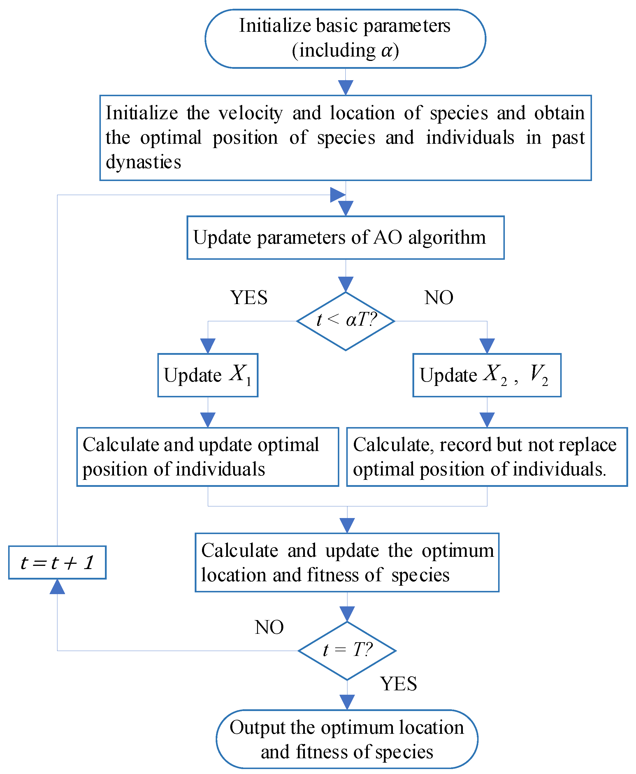
The PSO algorithm performs exploration well for solving nonlinear problems. However, it easily falls into local optima [21,22]. In this paper, a particle swarm aquila optimization (PSAO) algorithm is proposed by combining the characteristics of the PSO algorithm and AO algorithm aiming to perform deeper exploration and exploitation searches. In the first stage, the PSAO algorithm adopts the reduced development steps in the later stage of the algorithm to search the global optimal region in advance to prepare for finding the optimal solution. In the second stage, combined with the PSO algorithm, the velocity equation is introduced to explore the region, and the convergence speed is greatly accelerated to find the optimal solution. The specific steps of PSAO algorithm are as follows:

Stage 1 [13]:

$$\begin{array}{c}{X}_1(t+1)=QF(t)\times X_{best}(t)-(G_1\times X(t)\times rand)\\ -G_2\times Levy(D)+rand\times G_1\end{array}$$

(9)

where $X_1(t+1)$ is the individual position updated by stage 1 in generation $t+1$; $X(t)$ is the individual position of generation $t$; $QF(t)=t^{\frac{2\times rand-1}{{(1-T)}^2}}$; $G_1$ represents the movement position when tracking the prey; $G_1=2\times rand-1$; $G_2$ represents the flight rate of tracking prey, decreasing from 2 to 0; $G_2=2\times (1-\frac{t}{T})$.

$Levy(D)$ is the Levy flight distribution function with dimension $D$, which can be expressed as [13]:

$$Levy(D)=s\times \frac{u\times \sigma }{{\left|v\right|}^{\frac{1}{\beta }}}$$

(10)

where $s=0.01$, $u$ and $v$ are Gaussian-distributed random numbers obeying $N\left(0,{\sigma }^2\right)$, $N\left(0,1\right)$, $\sigma ={\left(\frac{\mathsf{\Gamma }(1+\beta )\times \sin (\frac{\pi \beta }{2})}{\mathsf{\Gamma }(\frac{1+\beta }{2})\times \beta \times 2(\frac{\beta -1}{2})}\right)}^{\frac{1}{\beta }}$ and $\beta =1.5$.

Stage 2:

$$\begin{array}{c}{V}_2(t+1)=(1-\frac{t}{T})\times V(t)+c_1\times rand\times (X_{ibest}(t)\\ -X(t))+c_2\times rand\times (X_{best}(t)-X(t))\end{array}$$

(11)

$$X_2(t+1)=X(t)+V_1(t+1)$$

(12)

where $V_2(t+1)$ is the particles’ velocity of generation $t+1$ in stage 2, $t$ is the current algebra and $T$ is the total number of iterations. $X_2(t+1)$ is the particles’ positions in generation $t+1$; $X_{ibest}$ represents the best positions of particles in previous dynasties; $X_{best}$ is the best particle position in the particle swarm; $rand$ is the inertia factor;$c_1$ and $c_2$ are the learning factors. The flow chart of the PSAO algorithm is shown in Figure 3.

In the first step, the PSAO algorithm initializes basic parameters and species. After that, it enters the loop iteration and begins to update the parameters which existed in stage 1. If current generation $t$ is less than $\alpha T$, the algorithm stays at stage 1. If not, the algorithm enters stage 2. When current generation $t$ equals the total number of iterations $T$, the algorithm is finished, and the optimum location and fitness of the species can be obtained.

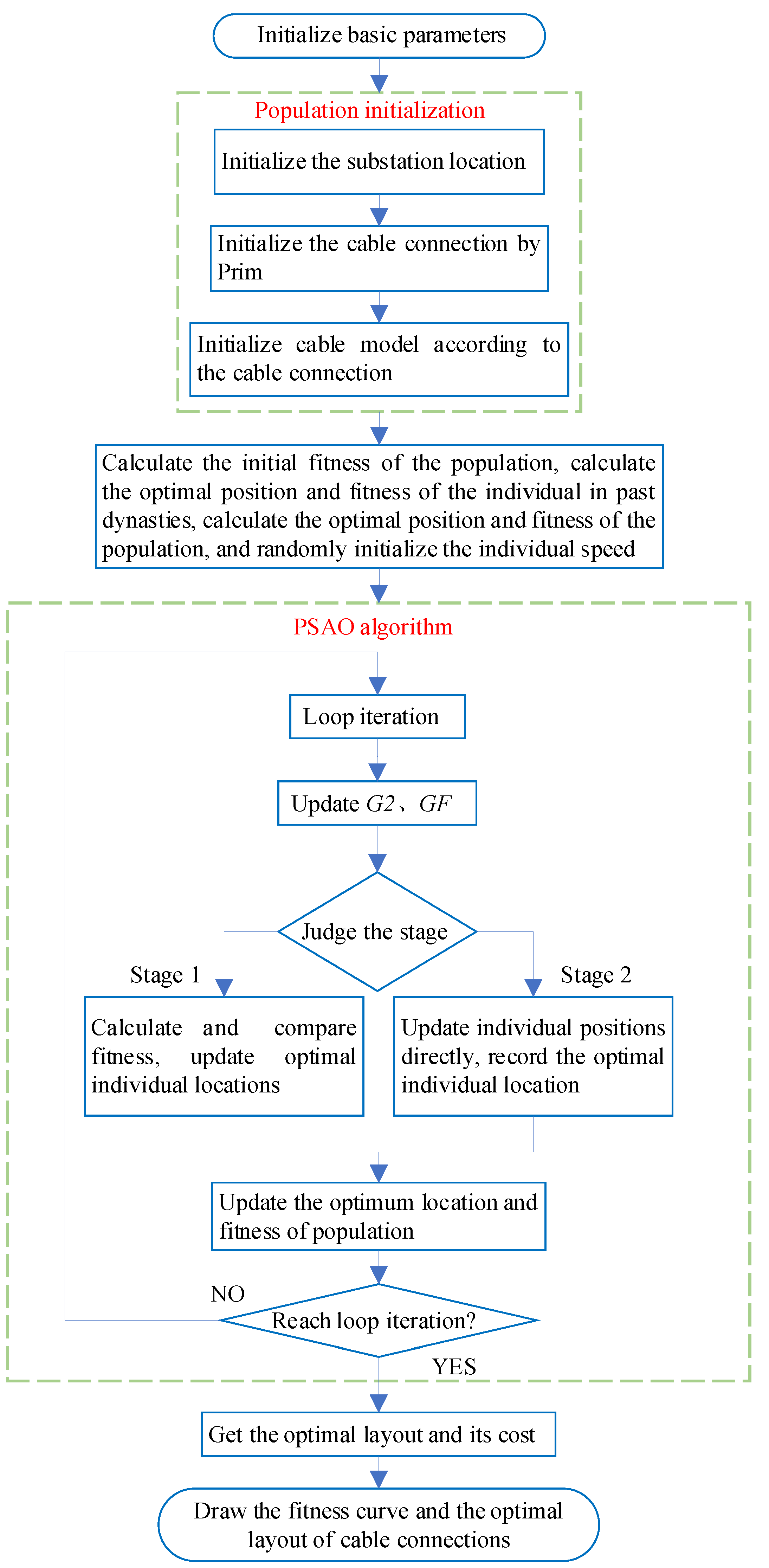
3.3.2. Algorithm Implementation

Basic parameters are initialized before solving. Then, the population is initialized by the Prim algorithm. After population initialization, the PSAO algorithm can be used to solve the optimization model, which has the steps described in the previous section. The total of cable investment cost, construction cost, and energy loss cost is taken as a fitness function and solved as an optimization objective of the algorithm. In the end, the optimal layout and its cost can be obtained. At the same time, a figure of fitness curve and a figure of the optimal layout of cable connections can be gained through the design. The process of model solving is shown in Figure 4.

4. Example Analysis

In this study, a real offshore wind farm in Guishan, Zhuhai, China, was selected for analysis, which has a power collection system to connect a substation with 27 wind turbines. The positions of wind turbines are given, and the best position for the substation needs to be decided on.

4.1. Data Selection for the Offshore Wind Farm

The parameters of the wind turbine are summarized in

Table 1. Parameters of the wind turbine.

Rated Capacity	Rotor Radius	Hub Height	Cut-in Wind Speed	Rated Wind Speed	Cut-out Wind Speed
10 MW	89.15 m	119 m	4 m/s	11.3 m/s	25 m/s

. These parameters are common to wind turbines in such a power collection system.

By converting the geographical locations of the wind turbines to the rectangular system, the layout is described in Figure 5.

The annual wind direction distribution in this region is shown in Figure 6. As it shows, northerly and southerly winds blow most of the time, and an easterly wind is very rare in this area.

For cable selection, the rated voltage of the power collection system was set to 35KV. The selected cables are classified by different cross-sectional areas, resistance, maximum ampacity and unit price. Additionally, the parameters of selected cables are all suitable for a power collection system running at 35 KV. The cable’s parameters are shown in

Table 2. Parameters of cables.

Cross-Sectional Area (mm2)	Resistance (Ω·km−1)	Maximum Ampacity (A)	The Unit Price (CNY·m−1)
50	0.387	175	980.99
95	0.913	255	1221.21
150	0.124	335	1491.48
240	0.0761	430	1771.79
400	0.0481	550	2302.33
500	0.0449	630	2811.33

.

4.2. Algorithm Optimization Results

To verify the superiority of PSAO, the AO algorithm, PSO algorithm and genetic algorithm (GA) were also used to solve this optimization problem. The parameters of each algorithm are shown in

Table 3. Parameters of algorithms.

GA	PSO	AO	PSAO
$P_c=0.7$	$c_1=2$	$r_1=10$	$c_1=2$
$P_m=0.1$	$c_2=2$ $w=0.9$	$\gamma =0.1$ $\beta =0.1$	$c_2=2$ $w=0.9$
		$G_2=2\times \left(1-\frac{t}{T}\right)$	$G_2=0.001$
		$QF={2000}^{(\frac{2\times rand-1}{{(1-2000)}^2})}$	$QF={2000}^{(\frac{2\times rand-1}{{(1-2000)}^2})}$
		$\alpha =0.1$	$\alpha =0.1$

.

4.2.1. Optimization Results of Substation Location

The number of iterations of each the three algorithms was set to 2000, and the population size was set to 100. The three algorithms were independently run 10 times in this study, and the simulation environment was Windows10, Intel(R) Core (TM) i5-8265u CPU@ 1.60 GHz, 1.80 GHz, 8 GB RAM. The statistical table of optimal solutions is

Table 4. Statistical table of optimal solutions.

Solution Type	Optimization Algorithm	Investment Cost (Per Million CNY)	Loss Cost (Per Million CNY)	Construction Cost (Per Million CNY)	Total Cost (Per Million CNY)
The optimal	GA	84.956	38.639	0.1993	123.795
	PSO	86.413	34.758	0.1996	121.371
	AO	85.756	35.521	0.1863	121.463
	PSAO	82.517	37.164	0.1863	119.867
The average	GA	87.629	40.473	0.1926	128.295
	PSO	89.912	35.218	0.1874	125.317
	AO	87.142	38.954	0.1886	126.286
	PSAO	85.267	36.661	0.1872	122.115
The worst	GA	86.396	47.957	0.1863	134.539
	PSO	87.466	40.628	0.1884	128.282
	AO	88.264	45.478	0.1994	133.942
	PSAO	83.929	40.458	0.1804	124.567

.

The box plots of total cost are shown in Figure 7. It can be seen that the total cost of the PSAO algorithm is lower than those of the other algorithms. Compared with the PSO algorithm, AO algorithm and GA, the average total cost of the PSAO algorithm was reduced by 2.6%, 3.3% and 4.8%, respectively. The PSAO algorithm has better optimization results for all costs than the AO algorithm and GA. Compared with the PSO algorithm, the optimization of cable investment cost was reduced by the PSAO algorithm, which makes the total cost achieved by the PSAO algorithm even lower than that achieved by PSO. For the optimal solution, the total cost of the PSAO algorithm was reduced by 1.2%, 1.3% and 3.2% compared with the PSO algorithm, AO algorithm and GA, respectively. For the worst solution, the total cost of the PSAO algorithm was reduced by 2.9%, 6.9% and 7.4% compared with the PSO algorithm, AO algorithm and GA, respectively. As for the fluctuation of the algorithm, the difference between the extreme value and the average value of the algorithm was divided by the average value for comparison. It can be concluded that the volatility of the AO algorithm was the highest, and its difference accounted for 3.8% or 6.0% of the average value. The GA had the second highest volatility, with the difference accounting for 3.5% or 4.9%. The PSO algorithm had a difference accounting for 3.2% or 2.4%. The PSAO algorithm had the least volatility, and its difference ratio was 1.8% or 2.0%.

The average solving time of each of the three algorithms is shown in the

Table 5. Solving time.

GA	PSO	AO	PSAO
982.61 s	863.36 s	923.42 s	872.14 s

. It can be seen that the GA and the AO algorithm both take a long time to solve; the PSO algorithm and PSAO algorithm are little different in solving time; and the PSO algorithm has the shortest solving time. The solving time of the PSAO algorithm was 1.02% more than that of the PSO algorithm. The solving time of the AO algorithm was 6.96% more than that of the PSO algorithm. The GA had the longest solving time, which was 12.67% more than that of the PSAO algorithm.

The fitness curves were solved by them together for comparison, as shown in Figure 8. It can be seen that the PSAO algorithm has a lower fitness value and faster convergence speed than the other algorithms. However, due to the characteristics of the PSAO algorithm exploring the global region in the first stage, the algorithm focuses on preparing for finding the optimal solution of the problem in the early stage, and its fitness curve declines slowly in the early stage. After the Prim algorithm was used to initialize the population, the PSO algorithm’s convergence declined rapidly in the early iterations, and the convergence algebra was later than that of the PSAO algorithm. As it is easy to fall into a local optimal solution, the optimization cost of the solution is high, and a better solution in the global scope was not found. The GA is similar to the PSO algorithm. The fitness value of the GA decreased rapidly in the early stage, but the algorithm fell into a local minimum point in the later stage. As for AO algorithm, because it can realize the smooth transition between the exploration stage and the development stage, it will not fall into a local optimal solution too early. Especially when solving multimodal problems, the AO algorithm has some advantages. The convergence curve of the algorithm appears like stairs, unlike those of other metaheuristic algorithms. This means that the fitness value may get lower if the number of iterations is more than two thousand or continuously increases. However, it takes a long time to find the global optimal solution. Due to the characteristics of the AO algorithm, its convergence speed is obviously worse than those of other algorithms, and the final optimization cost is higher than that of the PSAO algorithm.

The above analysis shows that the PSAO algorithm has obvious advantages in solving this optimization problem compared to other algorithms. The optimal cable connection topology of the power collection system solved by PSAO is obtained in Figure 9. It can be seen that the substation is roughly in the center of the wind farm area and there is no crossover between the cables of each wind turbine. It is worth mentioning that the cable selection in Figure 9 is not entirely based on the maximum ampacity available. The reason for that is the cable investment cost reduction will lead to an increase in the cost of energy loss.

4.2.2. Optimized Results Given Substation Location

In order to solve the optimization model, the location of the substation, the cable connections and the cable model are all selected as optimization variables. However, in practice, the location of the substation will also be selected. In order to better study the effectiveness of the PSAO algorithm for the cable connection layout of this model, the location of the substation was fixed to the coordinates (3500, 3000) in Figure 5, which is also roughly the center of the wind turbine cluster. The PSAO algorithm, PSO algorithm, AO algorithm and GA were used to solve the model in this situation, and the fitness curves are shown in Figure 10.

As can be seen in Figure 10, when the optimization variables are cable connection and cable selection, the PSAO algorithm still has advantages for solving this model. The optimization cost of the PSAO algorithm is lower than those of the other algorithms, and its convergence speed is faster and convergence algebra is earlier. The convergence rate of the PSO algorithm is faster in the early stage, and its convergence algebra is similar to that of the PSAO algorithm, but its local convergence characteristics make the optimization cost the highest. The optimization cost of the GA is slightly lower than that of the PSO algorithm. The fitness curve of the AO algorithm is still stair-shaped; its convergence speed is obviously slower than those of other algorithms, and the optimization cost is lower than those of the PSO algorithm and GA but higher than that of the PSAO algorithm. It can be seen that after the location of substation is given, the optimization costs of the four algorithms increase to a certain extent. The total costs of the GA, PSO algorithm, AO algorithm and PSAO algorithm increased by about 1.4%, 4.3%, 0.50% and 0.98%, respectively.

After the location of the substation was given, the PSAO algorithm was used to solve the model, and the cable connection topology of the power collection system is described in Figure 11. The substation was located at the coordinates (3500, 3000). It can be seen that the cable connection layout has a tree structure, and there are signs of wind turbine partition processing. There is no crossover between the cables of each wind turbine, so the overall connection is reasonable.

4.2.3. Algorithm Comparison Results

According to the simulation results of fixed substation and variable substation location, the four characteristics of the algorithms of convergence speed, volatility, solving time and accuracy are summarized, as shown in

Table 6. Comparison table of algorithms’ characteristics.

Optimization Algorithm	Convergence Speed	Volatility	Solving Time	Accuracy
GA	medium	high	long	low
PSO	medium	medium	short	medium
AO	slow	high	long	medium
PSAO	fast	low	medium	high

.

As for the GA, cross-operation easily produces infeasible solutions in this optimization problem, resulting in poor optimization ability of the algorithm. In addition, due to the existence of encoding and decoding parts, the algorithm takes a long time to solve the problem. The AO algorithm focuses on exploration, so the convergence speed is slow. The PSO algorithm had decent optimization performance, and the solving time of the PSO algorithm was the shortest. Therefore, using the AO algorithm to improve the search ability of the PSO algorithm in the early stage can further improve the algorithm’s performance. Experimental verification showed that the hybrid algorithm has the best optimization performance, and it is only slightly inferior to the PSO algorithm in terms of solving time. In summary, the PSAO algorithm has great advantages in solving the optimization problems of collector systems.

5. Conclusions

For the topological optimization of an offshore wind farm power collection system, we integrated cable investment, energy loss and line construction and established a cost model which has a certain reference value. To solve the problem, a method of wind turbine grouping has been proposed, and each group is initialized by the Prim algorithm separately considering the constraints. The PSAO algorithm was proposed to solve the problem. An example showed that the PSAO algorithm has a lower optimization cost than the PSO algorithm, AO algorithm and GA after Prim initialization. The results show that the PSAO algorithm still has excellent results and the lowest optimization cost when the power station’s location is (3500, 3000). In the future, different optimization variables can be selected to solve the problem, or wind turbine location and layout can be added to the optimization model.

References

1. Gao, X.; Li, L.; Zhang, S.; Zhu, X.; Sun, H.; Yang, H.; Wang, Y.; Lu, H. LiDAR-based observation and derivation of large-scale wind turbine’s wake expansion model downstream of a hill. Energy 2022, 259, 125051. [Google Scholar] [CrossRef]
2. Liu, J.; Song, D.; Li, Q.; Yang, J.; Hu, Y.; Fang, F.; Joo, Y.H. Life cycle cost modelling and economic analysis of wind power: A state of art review. Energy Convers. Manag. 2023, 277, 116628. [Google Scholar] [CrossRef]
3. Perez-Rua, J.-A.; Cutululis, N.A. Electrical Cable Optimization in Offshore Wind Farms—A Review. IEEE Access 2019, 7, 85796–85811. [Google Scholar] [CrossRef]
4. Marge, T.; Lumbreras, S.; Ramos, A.; Hobbs, B.F. Integrated offshore wind farm design: Optimizing micro-siting and cable layout simultaneously. Wind Energy 2019, 22, 1684–1698. [Google Scholar] [CrossRef] [Green Version]
5. Paul, S.; Rather, Z.H. A novel approach for optimal cabling and determination of suitable topology of MTDC connected offshore wind farm cluster. Electr. Power Syst. Res. 2022, 208, 107877. [Google Scholar] [CrossRef]
6. Hou, P.; Hu, W.; Soltani, M.; Chen, C.; Chen, Z. Combined optimization for offshore wind turbine micro siting. Appl. Energy 2017, 189, 271–282. [Google Scholar] [CrossRef]
7. Mokhi, C.E.; Addaim, A. Optimization of wind turbine interconnections in an offshore wind farm using metaheuristic algorithms. Sustainability 2020, 12, 5761. [Google Scholar] [CrossRef]
8. Zuo, T.; Zhang, Y.; Meng, K.; Tong, Z.; Dong, Z.Y.; Fu, Y. A Two-Layer Hybrid Optimization Approach for Large-Scale Offshore Wind Farm Collector System Planning. IEEE Trans. Ind. Inform. 2021, 17, 7433–7444. [Google Scholar] [CrossRef]
9. Wang, L.; Wu, J.; Wang, T.; Han, R. An optimization method based on random fork tree coding for the electrical networks of offshore wind farms. Renew. Energy 2020, 147, 1340–1351. [Google Scholar] [CrossRef]
10. Gonzalez-Longatt, F.M.; Wall, P.; Regulski, P.; Terzija, V. Optimal Electric Network Design for a Large Offshore Wind Farm Based on a Modified Genetic Algorithm Approach. IEEE Syst. J. 2012, 6, 164–172. [Google Scholar] [CrossRef]
11. Pillai, A.C.; Chick, J.P.; Johanning, L.; Khorasanchi, M. Offshore wind farm layout optimization using particle swarm optimization. J. Ocean. Eng. Mar. Energy 2018, 4, 73–88. [Google Scholar] [CrossRef] [Green Version]
12. Peng, H.; Hu, W.; Zhe, C. Optimisation for offshore wind farm cable connection layout using adaptive particle swarm optimisation minimum spanning tree method. IET Renew. Power Gener. 2016, 10, 694–702. [Google Scholar]
13. Abualigah, L.; Yousri, D.; Abd Elaziz, M.; Ewees, A.A.; Al-qaness, M.A.A.; Gandomi, A.H. Aquila Optimizer: A novel meta-heuristic optimization algorithm. Comput. Ind. Eng. 2021, 157, 107250. [Google Scholar] [CrossRef]
14. Jiang, Q.; Li, B.; Liu, T. Tech-Economic Assessment of Power Transmission Options for Large-Scale Offshore Wind Farms in China. Processes 2022, 10, 979. [Google Scholar] [CrossRef]
15. Wedzik, A.; Siewierski, T.; Szypowski, M. A new method for simultaneous optimizing of wind farm’s network layout and cable cross-sections by MILP optimization. Appl. Energy 2016, 182, 525–538. [Google Scholar] [CrossRef]
16. Srikakulapu, R.; Vinatha, U. Optimized design of collector topology for offshore wind farm based on ant colony optimization with multiple travelling salesman problem. J. Mod. Power Syst. Clean Energy 2018, 6, 1181–1192. [Google Scholar] [CrossRef] [Green Version]
17. Jin, R.; Hou, P.; Yang, G.; Qi, Y.; Chen, C.; Chen, Z. Cable routing optimization for offshore wind power plants via wind scenarios considering power loss cost model. Appl. Energy 2019, 254, 113719. [Google Scholar] [CrossRef]
18. Gao, X.; Zhang, S.; Li, L.; Xu, S.; Chen, Y.; Zhu, X.; Sun, H.; Wang, Y.; Lu, H. Quantification of 3D spatiotemporal inhomogeneity for wake characteristics with validations from field measurement and wind tunnel test. Energy 2022, 254, 124277. [Google Scholar] [CrossRef]
19. Jensen, N.O. A Note on Wind Generator Interaction; Technical Note Risø-M-2411; Risø National Laboratory: Roskilde, Denmark, 1983. [Google Scholar]
20. Katic, I.; Højstrup, J.; Jensen, N.O. A simple model for cluster efficiency. In European Wind Energy Association Conference and Exhibition; Technical University of Denmark: Lyngby, Denmark, 1986; pp. 407–410. [Google Scholar]
21. Kennedy, J.; Eberhart, R. Particle swarm optimization. In Proceedings of the ICNN’95—International Conference on Neural Networks, Perth, Australia, 27 November–1 December 1995. [Google Scholar]
22. Kennedy, J. The particle swarm: Social adaptation of knowledge. In Proceedings of the 1997 IEEE International Conference on Evolutionary Computation (ICEC ‘97), Indianapolis, IN, USA, 13–16 April 1997. [Google Scholar]
Figure 1. Schematic diagram of optimized variable coding.
Jmse 11 00279 g001
Figure 2. Schematic diagram of wind turbine grouping.
Jmse 11 00279 g002
Figure 3. The flow chart of particle swarm aquila optimization.
Jmse 11 00279 g003
Figure 4. The process of our method.
Jmse 11 00279 g004
Figure 5. The layout diagram of wind turbines in a coordinate plane.
Jmse 11 00279 g005
Figure 6. Wind rose diagram.
Jmse 11 00279 g006
Figure 7. Box plots of total cost.
Jmse 11 00279 g007
Figure 8. Fitness curve (variable substation location).
Jmse 11 00279 g008
Figure 9. The topology of cables’ connection (variable substation location).
Jmse 11 00279 g009
Figure 10. Fitness curve (given substation location).
Jmse 11 00279 g010
Figure 11. The topology of cables’ connection (given substation location).
Jmse 11 00279 g011