VFR: The Underwater Acoustic Target Recognition Using Cross-Domain Pre-Training with FBank Fusion Features

Abstract

Underwater acoustic target recognition is a hot research area in acoustic signal processing. With the development of deep learning, feature extraction and neural network computation have become two major steps of recognition. Due to the complexity of the marine environment, traditional feature extraction cannot express the characteristics of the targets well. In this paper, we propose an underwater acoustic target recognition approach named VFR. VFR adopts a novel feature extraction method by fusing three-dimensional FBank features, and inputs the extracted features into a residual network, instead of the classical CNN network, plus cross-domain pre-training to perform target recognition. The experimental results show that VFR achieves 98.5% recognition accuracy on the randomly divided ShipsEar dataset and 93.8% on the time-divided dataset, respectively, which are better than state-of-the-art results.

1. Introduction

In underwater acoustic signal processing, target recognition is an important research topic. Over the past few decades, underwater acoustic target recognition has relied mainly on professionally trained sonar operators. However, the recognition accuracy heavily depends on the objective environment and human’s physical and mental states.

Nowadays, deep learning is gradually applied to underwater acoustic target recognition. The feature extraction and neural network computation constitute the two major steps of the recognition. The extracted features include waveform features, time-frequency features, and auditory features. The popular feature extraction methods are Fourier transform (STFT) [1], discrete Wavelet transform (DWT) [2], LOFAR [3], DEMONs [4], Hilbert-Huang transform [5], Mel-frequency cepstral coefficient (MFCC) [6], Mel filterbank (FBank) [7] and so on. However, impacted by unfavorable factors such as the diversity of acoustic target and the complexity of marine environment, traditional factor extraction methods do not meet the demand of recognition accuracy. In terms of deep learning network architecture, various architectures such as CNN [8], RNN [9], DBN [10] have been applied to underwater target recognition systems.

This paper proposes a novel underwater acoustic target recognition approach named VFR. To target the diversity and complexity in underwater acoustic target recognition, VFR adopts a three-dimensional fusion feature. In terms of network architecture, VFR chooses a ResNet-18 network with cross-domain pre-training. The contributions of this paper can be summarized as follows,

• VFR fuses three-dimensional features from FBank, Delta FBank and Double-Delta FBank. Compared with the single dimensional feature obtained by traditional feature extraction methods, the fusion features better reflect the characteristics of underwater acoustic targets.
• VFR adopts the ResNet18 residual network architecture, rather than the commonly used classical CNN network, to avoid the neural degradation problem of traditional networks used in underwater acoustic target recognition. Combined with cross-domain pre-training, VFR effectively improves the recognition accuracy. In addition, pre-training enables VFR to save a great amount of training time.
• The experimental results show that VFR can achieve 98.5% recognition accuracy on the randomly divided ShipsEar dataset and 93.8% on the time-divided dataset, respectively, which, to the best of our knowledge, are the highest accuracy achieved.

2. Related Work

2.1. Feature Extraction Methods

In underwater acoustic target recognition, short-time Fourier transform (STFT), Mel cepstral coefficients (MFCC), and Mel filterbank (FBank) are three commonly used audio features in the feature extraction stage.

STFT is an extension of Fourier transform to address signal non-stationarity by applying windows for segmented analysis. In the continuous domain, STFT could be represented as

$$X(n,w)=\sum _{m=-\infty }^{\infty }x\left(m\right)g(n-m)e^{-jwn}$$

(1)

Here, $x\left(m\right)$ is the input signal, $g\left(m\right)$ is the window function, and $X(n,w)$ is a two-dimensional function of time n and frequency w.

FBank takes into account the human auditory characteristics. FBank first maps the linear spectrum to the Mel nonlinear spectrum based on auditory perception, and then converts it to the cepstrum. In Mel frequency domain, human perception of tones is linear. The essence of Mel filter is a scaling rule, which passes energy through a set of Mel scale triangle filter banks. FBank can be regarded as a system divides the input signal $x\left(m\right)$ into a set of analysis signals $x_1\left(m\right),x_2\left(m\right),\dots$, each of which corresponds to a different region in the spectrum of $x\left(m\right)$. It could be represented as

$$F_m={log}_{10}\sum _{k=0}^{N-1}{\omega }_M\left(k\right){\left|X\left(k\right)\right|}^2,0\le m\le M-1$$

(2)

Here, $X\left(k\right)$ is the FFT of input signal $x\left(m\right)$, the window function ${\omega }_m\left(k\right)$ is a Hanning window function, shown as follow:

$${\omega }_m\left(k\right)=\left\{\begin{array}{ll}0.5[1-cos(2\pi k/(M-1)],& 0\le k\le M-1\\ 0,& otherwise\end{array}\right.$$

(3)

MFCC also takes into account human perception for sensitivity at appropriate frequencies by converting the conventional frequency to Mel Scale. It could be represented as

$$C_m=\sum _{m=0}^{M-1}{F}_{m}cos(\pi n(m-0.5)/M),0\le n\le C-1$$

(4)

Here, C is the number of MFCCs.

Although STFT can retain the most comprehensive time-frequency information, it cannot highlight the spectral characteristics of the signal well. Both FBank and MFCC can highlight spectral features based on human hearing design, but the discrete cosine transform (DCT) in the MFCC method filters out part of the signal information and also increases the amount of calculation.

2.2. Deep Learning in Underwater Acoustic Target Recognition

The research on applying deep learning to underwater acoustic target recognition focus on three aspects:

The first is to enlarge the dataset of underwater acoustic. Attribute to military confidentiality and security reasons, the collection and production of dataset are difficult, and the existing data of underwater acoustic is scarce. However, deep learning needs a large dataset for training, testing and validation. Data enhancement [11] technology has been used to expand existing underwater acoustic data to meet the needs of large data volumes in deep learning. Jin et al. [12] and Gao et al. [13] apply Generative Adversarial Networks (GAN) to enlarge the underwater acoustic dataset. Luo et al. [14] improves classification recognition rates by using a conditional Generative Adversarial Network(cGAN) to amplify the original data samples.

The second is to apply deep learning to underwater acoustic target recognition, besides other classical deep learning fields (such as computer vision, natural language recognition, etc.). Hu et al. [15], Sun et al. [16], etc., use the traditional time domain feature as the input of the deep learning networks. These studies focus on design and optimization of deep neural network architectures. They use original signal dimensional data without pre-processing, which potentially reduces the recognition accuracy could be achieved.

The third is the data pre-processing before input to the neural network. Because of the environmental noise pollution and the limitation of the format of the collected data, the dataset should be denoised and transformed. Feature extraction makes the input single dimensional data more suitable for deep learning network process. Some feature extraction studies are referred to [16,17,18]. Sun et al. [16] uses real-valued and complex-valued ResNet and DenseNet convolutional networks to recognize synthetic mixed multitarget signals with various features. Liu et al. [17] adopted fusion Mel Spectrum, and use the LSTM model to improve recognition accuracy. Hong et al. [18] fuses Log-Mel Spectrogram (LM), MFCC, and CCTZ (the composition of Chroma, Contrast, Tonnetz, and Zero-cross ratio) features and data augmentation with 16-layer Residual Network for underwater acoustic recognition problems. Our work are inspired by these approaches.

2.3. Pre-Training

Pre-training [19] is widely used in the fields of computer vision, natural language processing and speech. For example, supervised ImageNet pretrained models are widely used for object detection and segmentation tasks.

When training the neural network, it is generally based on the back-propagation algorithm. First, the parameters in the network are randomly initialized, and then optimization algorithms such as stochastic gradient descent (SGD) are used to continuously optimize the model parameters. As a comparison, pre-training trains the model parameters through some given tasks, and then uses the resulting parameters to initialize the model rather than using randomly initialized ones.

3. Methodology

In this section, we first give an overview of VFR architecture, and then give a detailed description on the following: FBank feature extraction method, the structure of residual network ResNet18, and the cross-domain pre-training.

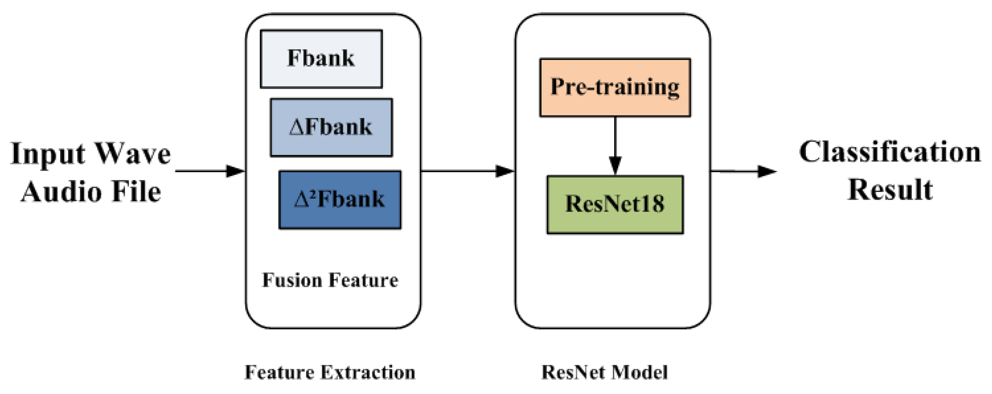
3.1. System Overview

In VFR, we use FBank, delta FBank and delta-delta FBank to construct a fusion feature; taking the feature as input, we classify and recognize the target based on the model constructed by a residual network ResNet18. The architecture of VFR is shown in Figure 1.

3.2. Feature Extraction

As mentioned above, STFT can retain the most comprehensive time-frequency information, but cannot express the spectral characteristics of the signal well. Both FBank and MFCC are based on spectral features extracted from human hearing features, but the DCT in MFCC will bring more signal distortion. In terms of retaining the time-frequency information, FBank also presents the spectral features of the signal as much as possible and thus is considered to be a better feature extraction method in underwater acoustic target recognition. Therefore, we choose FBank as the base feature in VFR.

However, in the underwater acoustic target recognition, the information contained in the traditional one-dimensional extracted features can not express the characteristics well. Simply using FBank as input is not able to achieve desired recognition accuracy because it can only reflect the static characteristics of the signal and cannot reflect the timing characteristics.

The delta feature has been proved to be an efficient supplementary to the original feature to improve recognition accuracy [20]. This is because the original spectral feature can only reflect the static characteristics of the signal and cannot reflect the timing characteristics. By calculating the delta feature, it is possible to obtain adjacent dynamic characteristics of the frame. For a short-time cepstral sequence $C\left[n\right]$, the delta-cepstral features are typically defined as

$$D\left[n\right]=C[n+m]-C[n-m]$$

(5)

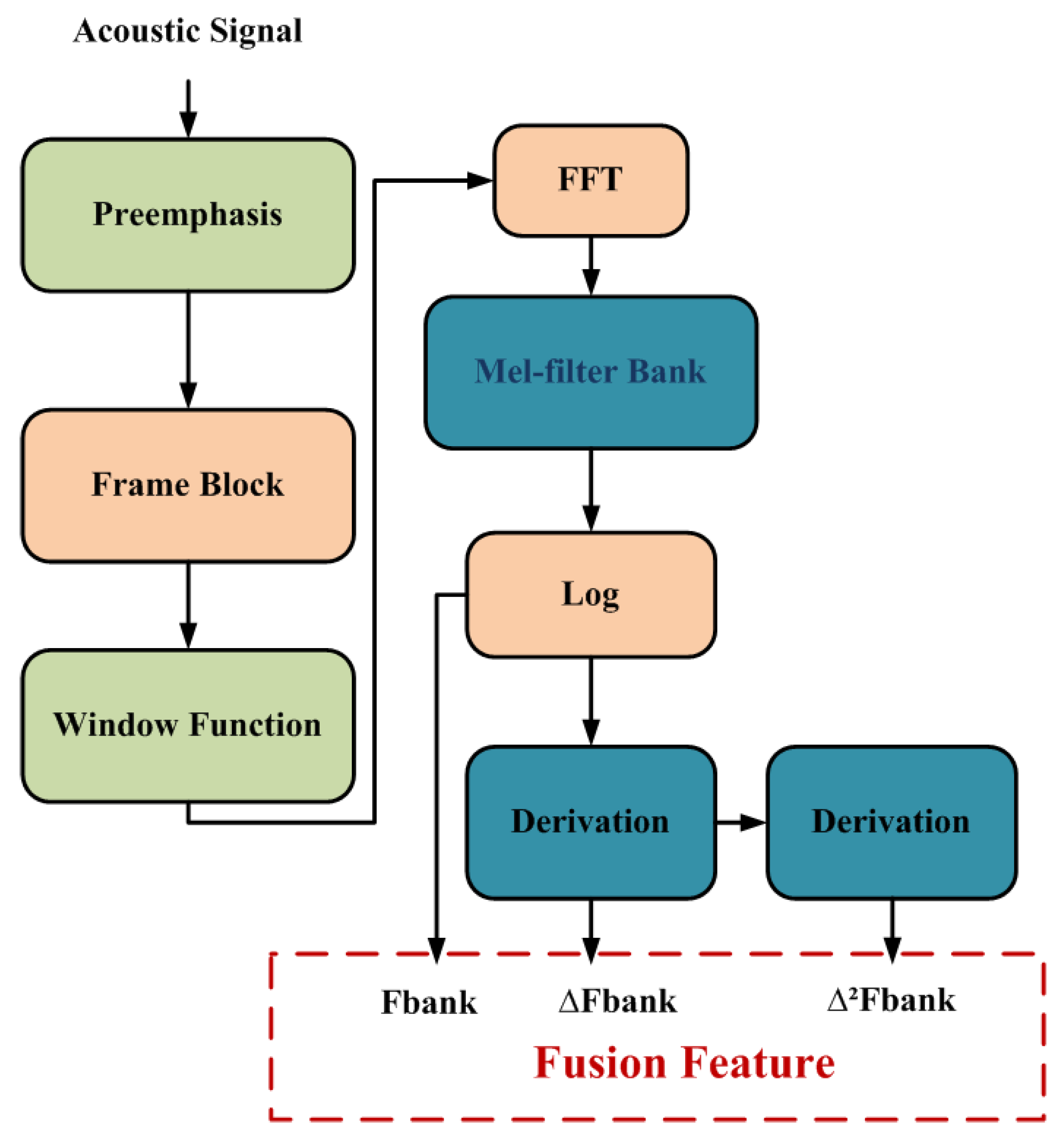
where n is the index of the analysis frames and in practice m is approximately 2 or 3. Similarly, double-delta cepstral features are defined in terms of a subsequent delta-operation on the delta-cepstral features. Therefore, VFR adopts delta method, utilizing FBank, delta FBank and double-delta FBank to construct a fusion spectral feature as input to the model.

In subsequent experiments, the fusion spectral future can be expressed as $R^{C\times F\times T}$. Here, C represents the dimension of the spectral feature, F represents the number of Mel filters in the frequency dimension, and T represents the length of the output in the time dimension. We show the fusion feature extraction pipeline in detail in Figure 2.

3.3. The ResNet18 Network

As the network becomes deeper and deeper, the training becomes harder and the optimization of the network becomes more and more difficult. In theory, the deeper the network, the better the effect should be; however, in fact, due to the difficulty of training, the network that is too deep will cause degradation problems, and the effect is not as good as the relatively shallow network. When it is stacked to a certain network depth, a vanishing gradient or exploding gradient problem may appear. As the network becomes deeper in underwater acoustic target recognition, problems as previously mentioned can be mitigated by adding by adding a residual module [21]. The residual module adds short connections based on a single connection method. Short connections can span several layers, even are added to the input to directly map the input to the output, so as to avoid neural network degradation. Figure 3 shows the basic structure of the residual module, and we use ResNet18 as the network architecture to implement VFR.

VFR adopts a ResNet18 network as shown in Figure 4. There are four basic units, one convolutional layer and one fully connected layer. It has a total of 18 layers. The classical CNN network architecture with a convolution layer and pooling layer is shown in Figure 5.

3.4. Cross-Domain Pre-Training

VFR adopts cross-domain pre-training using image data ImageNet [22], which is proved to efficiently improve recognition accuracy. The improvement of recognition accuracy mainly comes from the overlap of underwater acoustic data feature spectrum and image information.The dataset of underwater acoustic is limited, and the large number of dataset in cross-domain pre-training can supplement the shortage of data. In addition, pre-training enables VFR to save great amount of training time.

ImageNet is an image dataset in the field of computer vision and is currently the largest database for image recognition in the world. The dataset has 1000 classes and contains 1,281,167 training images, 50,000 validation images, and 100,000 test images. It has become a recognized benchmark and pre-training model in the field of vision, and a large number of scholars have also done a lot of research work on it, such as AlexNet, VGG, ResNet, Inception, and many other neural network models.

In the implementation, we choose ResNet18 officially trained by pytorch as our pre-training model, with a top@1 of 69.758% and a top@5 of 89.078%. When we conduct experiments, we change the output of the ResNet18 model to the number of classifications in the target dataset, load the parameters of the pretrained model, and then train and fine-tune the entire ResNet18 network.

4. Experiments and Analysis

In this section, we introduce the dataset and the data processing methods. In addition, we analyze the experimental results.

4.1. Dataset and Dat Processing

The dataset used in our experiments is ShipsEar [23], which was recorded using digitalHyd SR-1 recorders at the port of Vigo, Spain in the autumn of 2012 and summer of 2013, with a total of 90 sound records and 11 vessel targets. The bandwidth of the signals is 25.8 KHz, and the sampling frequecy is 52.734 KHz. The duration of each recording varies from 15 s to 10 min. According to the size of the vessel, it can be divided into five categories (four vessel classes and one background noise class). The division method and the number of files are described in detail in

Table 1. The detail of the ShipsEar dataset.

Class	Type of Vessel
A	fishing boats, trawlers, mussel boats, tugboats and dredgers
B	motorboats, pilot boats and sailboats
C	passenger ferries
D	ocean liners and ro-ro vessels
E	background noise

. ShipsEar has been widely used in various studies and has become a recognized benchmark in the field of underwater acoustic target recognition.

In our experiments, we split the sound file into data samples with a time interval of 5 s. After removing some useless sound clips, 2251 data samples are obtained. When the model is trained, we use the following two data set division methods: (1) In the first method, each 5 s sound clip is regarded as an independent sample, and all the samples are divided into the training set, validation set, and test set according to the ratio of 7:1.5:1.5. Dataset A is obtained by this division method. (2) In the second division method, the original sound files are sorted in chronological order. The first 70% of them is the training set, and the remaining is divided into the validation set and the test set according to the ratio of 1:1. Dataset B is obtained by this data division. Finally, the number of samples in our training set, validation set, and test set are 1577, 336, and 338, respectively.

It should be pointed out here that Dataset B is more challenging in recognition tasks than Dataset A, and it is also more suitable for practical applications. This is because Dataset A does not consider the impact of the time dimension when dividing the data, while Dataset B is divided on a time-series basis, just like the real world, using samples of objects that have appeared in the past to predict upcoming objects.

4.2. Experimental Setup

On the two datasets divided in Section 4.1, first we use the classical CNN and reset18 models to perform preliminary performance evaluations on the three feature extraction methods as our benchmark baseline. Next, we use fusion spectral feature as the input of the neural network to observe and compare the performance of the fusion features in the recognition model. Finally, we use the cross-domain pre-training method to use ResNet18 trained on ImageNet as the initialization parameters of our model to study the final performance metrics.

4.3. Implementation Details

In our work, all experiments are done on a workstation, and the detailed hardware and software parameters are shown in the

Table 2. The configuration of the workstation.

Hardware/Software	Parameters/Version
CPU	Intel Xeon 4210R 2.40 GHz × 2
GPU	NVIDIA RTX3090 24 GB
Memory	128 GB
OS	Debian 11.4
Linux Kernel	5.10
Python	3.9.7
Pytorch	1.8.1

. During training, we set the batch size and the maximum number of epochs to 32 and 100, respectively. The cross-entropy loss function and Adam optimizer were used. The initial learning rate was set to ${10}^3$. We saved the model with the highest recognition accuracy and use the test set to verify the final recognition accuracy of this model.

In addition, the specific parameters of the classical CNN model and ResNet18 model used as a comparative experiment are as follows:

For the classical CNN model, we use two convolutional layers, one dropout layer set to 0.1, and two fully connected layers with softmax activation function. More specifically, the components of the first convolutional layer include in_chanels (1), out_chanels (64), kernel_size (5), stride (1), padding (2), activation function (Tanh), and maximum pooling (2); and the components of the second convolutional layer include in_chanels (64), out_chanels (256), kernel_size (5), stride (1), padding (2), activation function (Tanh), and maximum pooling (2).

The ResNet18 network structure we use is shown in Figure 4 with the input changed to 1 or 3 according to the number of channels of the input spectrum, the other structures remain unchanged.

4.4. Evaluation Indicators

In order to better evaluate the entire model, we use the accuracy, precision, recall, and F1-score as performance evaluation indicators. The calculation methods of each indicator are as follows:

$$\begin{array}{cc}\hfill \mathrm{accuracy}& =\frac{n_{AA}+n_{BB}+n_{CC}+n_{DD}+n_{EE}}{N}\hfill \end{array}$$

(6)

$$\begin{array}{cc}\hfill {\mathrm{precision}}_i& =\frac{n_{ii}}{n_{Ai}+n_{Bi}+n_{Ci}+n_{Di}+n_{Ei}}\hfill \end{array}$$

(7)

$$\begin{array}{cc}\hfill {\mathrm{recall}}_i& =\frac{n_{ii}}{n_{iA}+n_{iB}+n_{iC}+n_{iD}+n_{iE}}\hfill \end{array}$$

(8)

$$\begin{array}{cc}\hfill {\mathrm{F}1\text{-}\mathrm{score}}_i& =\frac{2\times {\mathrm{precision}}_i\times {\mathrm{recall}}_i}{{\mathrm{precision}}_i+{\mathrm{recall}}_i}\hfill \end{array}$$

(9)

In the above calculation method, N represents the total number of samples, and $n_{ij}$ represents the number of samples of class i that are predicted to be samples of class j.

When calculating the average value of each indicator, we use the macro calculation method. The specific calculation method is as follows:

$$\begin{array}{cc}\hfill \mathrm{macro}\text{-}P& =\frac{1}{n}\sum _{i=1}^n{P}_i\hfill \end{array}$$

(10)

$$\begin{array}{cc}\hfill \mathrm{macro}\text{-}R& =\frac{1}{n}\sum _{i=1}^n{R}_i\hfill \end{array}$$

(11)

$$\begin{array}{cc}\hfill \mathrm{macro}\text{-}\mathrm{F}1& =\frac{2\times \mathrm{macro}\text{-}P\times \mathrm{macro}\text{-}R}{\mathrm{macro}\text{-}P+\mathrm{macro}\text{-}R}\hfill \end{array}$$

(12)

4.5. Experimental Results

4.5.1. Comparison of Feature Extraction Methods

Table 3. The accuracy of different feature extraction methods.

Feature	CNN	ResNet18
STFT	0.778	0.769
FBank	0.840	0.938
MFCC	0.902	0.938
Fusion-STFT	0.769	0.527
Fusion-MFCC	0.905	0.932
Fusion-FBank	0.849	0.950

shows the recognition accuracy of three different feature extraction methods in two network architectures. The value of K (number of DFT points) is 254, N (number of MEL bands) is 128 and C (number of MFCCs) is 128. As shown in this table, we can see that in traditional single features, the performance of STFT is worse than that of FBank and MFCC. Under classical CNN model, the recognition accuracy of STFT is 6.2% and 22.4% lower than that of FBank and MFCC, respectively. In the ResNet18 network, the gap is further widened, and STFT is 26.9% lower than the other two methods, which corresponds to the fact that STFT cannot describe the spectral characteristics of the signal well. Overall, when we use the fusion features of delta and double-delta, the FBank spectrum is 0.9% and 1.2% higher than that of single features on classical CNN and ResNet18 models, respectively, and MFCC is 0.3% higher than single feature on classical CNN, and 0.6% lower on ResNet18 model. Among them, the FBank spectrum achieves a recognition accuracy of 95% in ResNet18 model, which is better than state-of-the-art results.

4.5.2. Comparison of Pre-Training

Section 4.5.1 shows that we can improve the recognition accuracy by using fusion features, and we need to combine the following cross-domain pre-training to further improve the performance of VFR.

In

Table 4. The recognition accuracy of three feature extraction methods before and after using pre-training.

Feature	Dataset A	Dataset B
Fusion-STFT	0.521	0.589
Fusion-MFCC	0.970	0.926
Fusion-FBank	0.979	0.905
Fusion-STFT + ImageNet	0.692	0.615
Fusion-MFCC + ImageNet	0.959	0.911
VFR (Fusion-FBank + Imagenet)	0.985	0.938

, we list the performance comparison of fusion features with and without pre-training on the ResNet18 model. In the datasets obtained by the two partitioning methods, the performance of fusion STFT and VFR has been improved to a certain extent. After pre-training, the recognition accuracy rates of the two were increased by 17.1% and 0.6% on dataset A, respectively; in dataset B, they were increased by 2.6% and 3.3%, respectively. The performance of fusion MFCC features decreases to a certain extent after pre-training, mainly because some signal details are lost after DCT calculation. After cross-domain pre-training, the best performance was achieved on the recognition task—98.5% for dataset A and 93.8% for dataset B.

4.5.3. Results Analysis

Table 5. The accuracy of different models.

Model	Dataset A	Dataset B
Baseline [23]	0.754	-
CNN	0.849	0.405
ResNet18	0.950	0.855
ResNet + Data Augmentation [18]	0.943	-
LSTM [17]	0.742	0.706
CRNN-9 [17]	0.946	0.873
cDCGAN [14]	0.963	0.929
VFR	0.985	0.938

compares VFR in terms of the recognition accuracy with previous studies using the ShipsEar dataset. As the results shown, VFR achieved 98.5% and 93.8% on datasets A and B, respectively. The recognition accuracy, as far as we know, is the best result currently available. On dataset A, this result far exceeds the baseline by 23.1%.

On the classical CNN model we described in the previous chapter, we achieved 84.9% recognition accuracy on dataset A, while the recognition accuracy on dataset B was only 40.5%. This experimental result shows that the classical CNN network cannot generalize the performance of the model on data set A to data set B, and the dimension of time has a great influence on the generalization ability of the model. VFR outperforms classical CNN by 13.6% and 53.4%, respectively.

On the ResNet18 model we described, the recognition accuracy rates of dataset A and dataset B are 95.0% and 85.5%, respectively. As the results shown, the accuracy has been greatly improved compared to the classical CNN, especially on dataset B(45%). With pre-training, the recognition accuracy is further improved by 3.5% and 8.3%, respectively, on the two datasets.

Liu et al. [17] adopted fusion Mel Spectrum, and use the LSTM model to achieve 74.2% and 70.6% recognition accuracy on data set A and dataset B, respectively, and 94.6% and 87.3% using the CRNN-9 model. Luo et al. [14] used CGAN to obtain classification recognition rates of 96.3% and 92.9% respectively after amplifying the original data samples. The highest recognition rates in these studies are also 2.2% and 0.9% lower than VFR, respectively.

To better demonstrate the performance of our model, we put accuracy, precision, recall and support (the number of samples in the test) in

Table 6. The results of each class on Dataset A.

Class	Accuracy	Precision	Recall	F1-Score	Support
A	0.982	1.000	0.982	0.991	56
B	0.957	0.957	0.957	0.957	47
C	0.984	0.984	0.984	0.984	127
D	1.000	0.987	1.000	0.993	74
E	1.000	1.000	1.000	1.000	34
Average	0.985	0.985	0.985	0.985	338

and

Table 7. The results of each class on Dataset B.

Class	Accuracy	Precision	Recall	F1-Score	Support
A	0.895	0.911	0.895	0.903	57
B	0.917	0.957	0.917	0.936	48
C	0.929	0.944	0.929	0.937	127
D	0.972	0.909	0.972	0.940	72
E	1.000	1.000	1.000	1.000	34
Average	0.938	0.944	0.943	0.943	338

. From the data, it can be seen that both Recall and Precision have reached a relatively high level. The division of dataset B is closer to the actual application scenario. Dataset B takes into account the timing characteristics of underwater acoustic signals, and uses previous data training to identify the types of signals that will appear soon.

5. Conclusions

In this paper, We propose a novel underwater acoustic target recognition approach named VFR. VFR chooses FBank as the base feature, and further adopts the delta method to obtain fusion feature as input to the network. Compared with the single dimensional feature obtained by traditional feature extraction methods, the fusion features better reflect the characteristics of underwater acoustic targets. VFR adopts the ResNet18 residual network architecture to avoid neural degradation problem. With cross-domain pre-training, VFR achieves the highest accuracy on the commonly used ShipsEar dataset, compared to the state of the art approaches.

References

- Seok, J.; Bae, K. Target Classification Using Features Based on Fractional Fourier Transform. IEICE Trans. Inf. Syst. 2014, E97.D, 2518–2521. [Google Scholar] [CrossRef]
- Azimi-Sadjadi, M.R. Underwater Target Classification Using Wavelet Packets and Neural Networks. IEEE Trans. Neural Netw. 2000, 11, 11. [Google Scholar] [CrossRef] [PubMed]
- van Haarlem, M.P. LOFAR: The Low Frequency Array. EAS Publ. Ser. 2005, 15, 431–444. [Google Scholar] [CrossRef]
- Pezeshki, A.; Azimi-Sadjadi, M.R.; Scharf, L.L. Undersea Target Classification Using Canonical Correlation Analysis. IEEE J. Ocean. Eng. 2007, 32, 948–955. [Google Scholar] [CrossRef]
- Adam, O. The Use of the Hilbert-Huang Transform to Analyze Transient Signals Emitted by Sperm Whales. Appl. Acoust. 2006, 67, 1134–1143. [Google Scholar] [CrossRef]
- Lim, T.; Bae, K.; Hwang, C.; Lee, H. Classification of Underwater Transient Signals Using MFCC Feature Vector. In Proceedings of the 2007 9th International Symposium on Signal Processing and Its Applications, Sharjah, United Arab Emirates, 12–15 February 2007; pp. 1–4. [Google Scholar] [CrossRef]
- Lim, Y. A digital filter bank for digital audio systems. IEEE Trans. Circuits Syst. 1986, 33, 848–849. [Google Scholar] [CrossRef]
- Smirnov, E.A.; Timoshenko, D.M.; Andrianov, S.N. Comparison of Regularization Methods for ImageNet Classification with Deep Convolutional Neural Networks. AASRI Procedia 2014, 6, 89–94. [Google Scholar] [CrossRef]
- Jozefowicz, R.; Zaremba, W.; Sutskever, I. An Empirical Exploration of Recurrent Network Architectures. In Proceedings of the International Conference on Machine Learning, Lille, France, 6–11 July 2015. [Google Scholar]
- Yue, H.; Zhang, L.; Wang, D.; Wang, Y.; Lu, Z. The Classification of Underwater Acoustic Targets Based on Deep Learning Methods. In Proceedings of the 2017 2nd International Conference on Control, Automation and Artificial Intelligence (CAAI 2017), Sanya, China, 25–26 June 2017. [Google Scholar] [CrossRef]
- Park, D.S.; Chan, W.; Zhang, Y.; Chiu, C.C.; Zoph, B.; Cubuk, E.D.; Le, Q.V. SpecAugment: A Simple Data Augmentation Method for Automatic Speech Recognition. arXiv 2019, arXiv:1904.08779. [Google Scholar]
- Jin, G.; Liu, F.; Wu, H.; Song, Q. Deep learning-based framework for expansion, recognition and classification of underwater acoustic signal. J. Exp. Theor. Artif. Intell. 2020, 32, 205–218. [Google Scholar] [CrossRef]
- Gao, Y.; Chen, Y.; Wang, F.; He, Y. Recognition Method for Underwater Acoustic Target Based on DCGAN and DenseNet. In Proceedings of the 2020 IEEE 5th International Conference on Image, Vision and Computing (ICIVC), Beijing, China, 10–12 July 2020. [Google Scholar]
- Luo, X.; Zhang, M.; Liu, T.; Huang, M.; Xu, X. An Underwater Acoustic Target Recognition Method Based on Spectrograms with Different Resolutions. J. Mar. Sci. Eng. 2021, 9, 1246. [Google Scholar] [CrossRef]
- Hu, G.; Wang, K.; Peng, Y.; Qiu, M.; Shi, J.; Liu, L. Deep Learning Methods for Underwater Target Feature Extraction and Recognition. Comput. Intell. Neurosci. 2018, 2018, 1214301. [Google Scholar] [CrossRef] [PubMed]
- Sun, Q.; Wang, K. Underwater Single-Channel Acoustic Signal Multitarget Recognition Using Convolutional Neural Networks. J. Acoust. Soc. Am. 2022, 151, 2245–2254. [Google Scholar] [CrossRef] [PubMed]
- Liu, F.; Shen, T.; Luo, Z.; Zhao, D.; Guo, S. Underwater Target Recognition Using Convolutional Recurrent Neural Networks with 3-D Mel-spectrogram and Data Augmentation. Appl. Acoust. 2021, 178, 107989. [Google Scholar] [CrossRef]
- Hong, F.; Liu, C.; Guo, L.; Chen, F.; Feng, H. Underwater Acoustic Target Recognition with a Residual Network and the Optimized Feature Extraction Method. Appl. Sci. 2021, 11, 1442. [Google Scholar] [CrossRef]
- Han, X.; Zhang, Z.; Ding, N.; Gu, Y.; Liu, X.; Huo, Y.; Qiu, J.; Yao, Y.; Zhang, A.; Zhang, L.; et al. Pre-trained models: Past, present and future. AI Open 2021, 2, 225–250. [Google Scholar] [CrossRef]
- Kumar, K.; Kim, C.; Stern, R.M. Delta-Spectral Cepstral Coefficients for Robust Speech Recognition. In Proceedings of the 2011 IEEE International Conference on Acoustics, Speech and Signal Processing (ICASSP), Prague, Czech Republic, 22–27 May 2011; pp. 4784–4787. [Google Scholar] [CrossRef]
- He, K.; Zhang, X.; Ren, S.; Sun, J. Deep Residual Learning for Image Recognition. In Proceedings of the 2016 IEEE Conference on Computer Vision and Pattern Recognition (CVPR), Las Vegas, NV, USA, 27–30 June 2016; pp. 770–778. [Google Scholar] [CrossRef]
- Deng, J.; Dong, W.; Socher, R.; Li, L.J.; Li, K.; Fei-Fei, L. ImageNet: A Large-Scale Hierarchical Image Database. In Proceedings of the CVPR09, Miami, FL, USA, 20–25 June 2009. [Google Scholar]
- Santos-Domínguez, D.; Torres-Guijarro, S.; Cardenal-López, A.; Pena-Gimenez, A. ShipsEar: An Underwater Vessel Noise Database. Appl. Acoust. 2016, 113, 64–69. [Google Scholar] [CrossRef]