
An Adversarial Single-Domain Generalization Network for Fault Diagnosis of Wind Turbine Gearboxes

 ,
,  and
and
Abstract
:1. Introduction
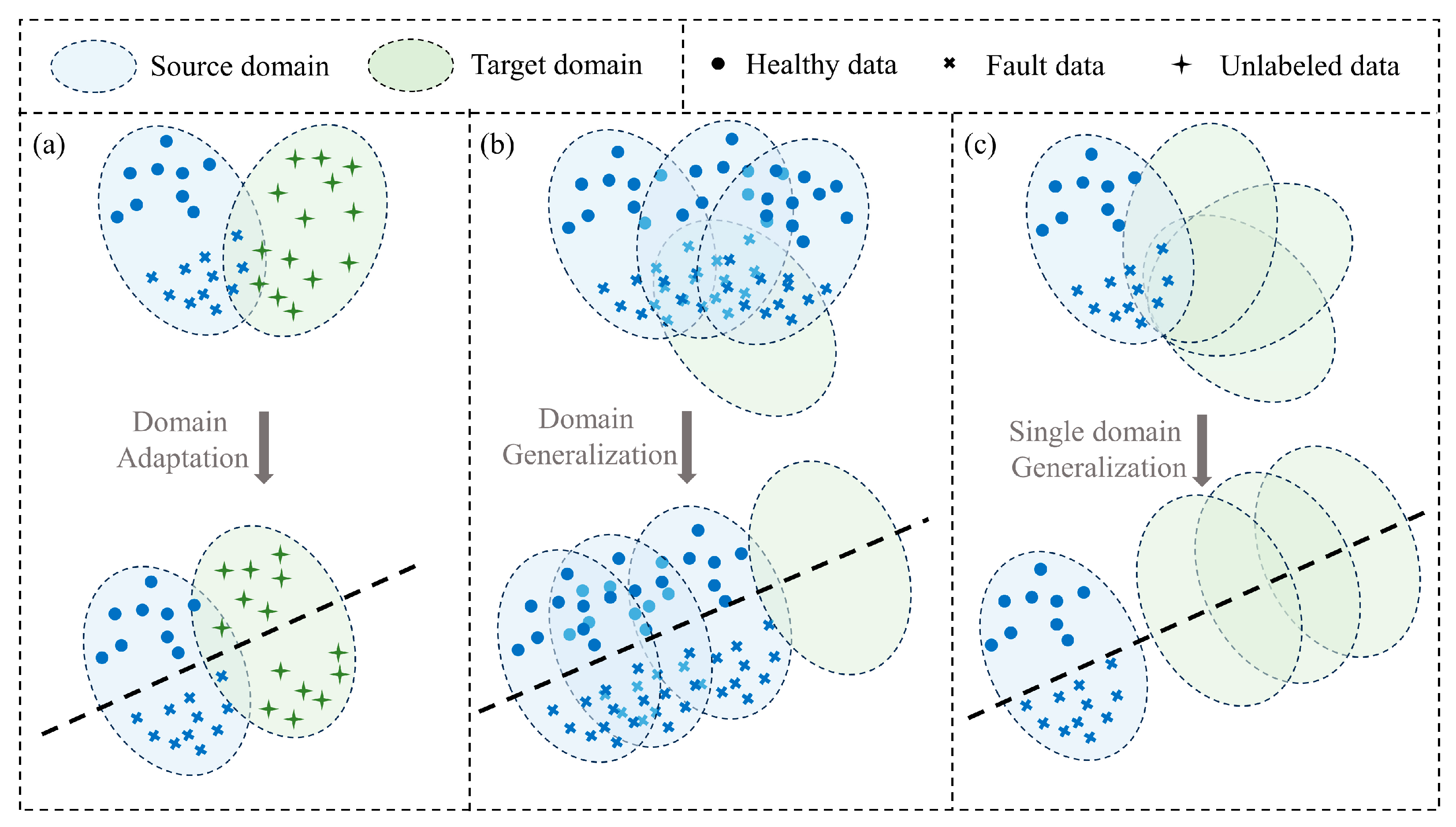
2. Related Work
3. Proposed Method
3.1. Problem Definition
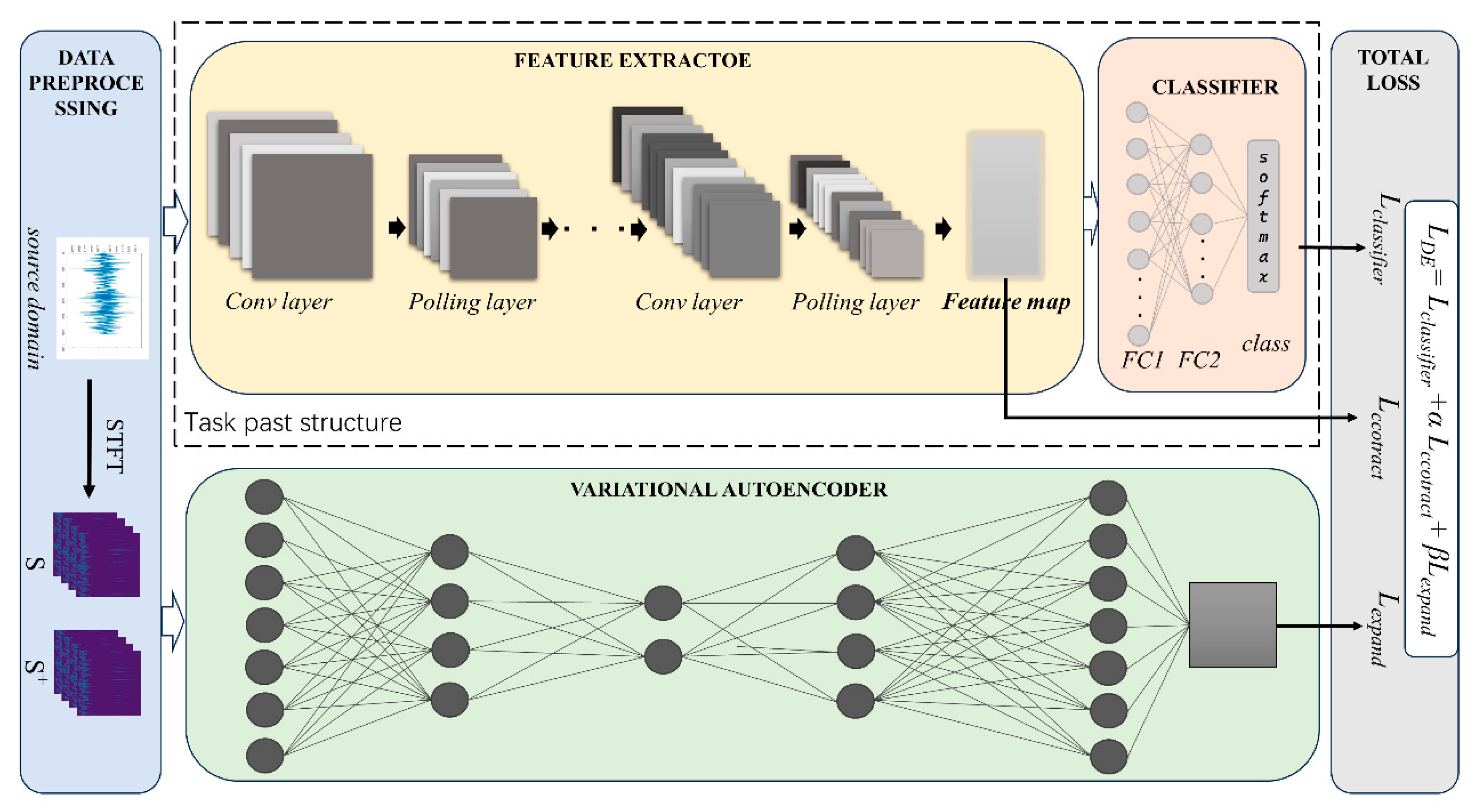
3.2. Structure
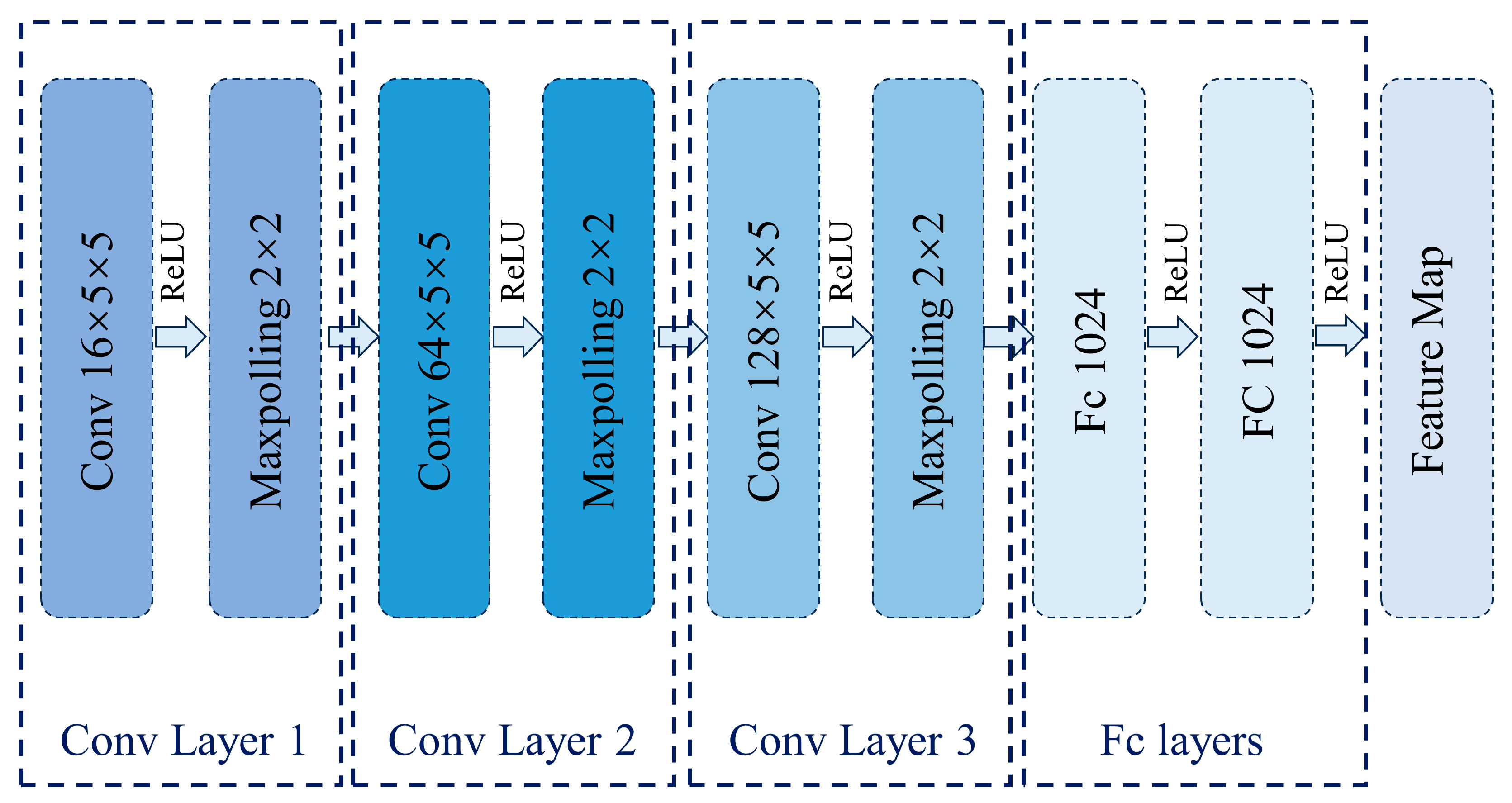
3.3. Feature Extractor
3.4. Variational Autoencoder
3.5. Model Optimization
| Algorithm 1. ASDGN |
| #Pre-train VAE |
| Input: Source dataset ; VAE model ; pre-train epoch E1 |
| for i = 1 to E1 do: |
| Randomly sample from S |
| Forward propagation and calculation Equation (7) |
| Backward propagation to update θ by Equation (9) |
| end |
| Return: pre-trained VAE model |
| #Domain Augmentation |
| Input: Source dataset ; pre-trained VAE model ; pre-trained feature extractor F; classifier C; number of augmentation domains K; Adversarial train epoch E2 |
| for i = 1 to K do: |
| for i = 1 to E2 do: |
| Randomly sample m data from S; |
| Forward propagation and calculation Equations (2), (5) and (8) |
| Calculation Equation (3) |
| Backward propagation to update by Equation (9) end |
| Create |
| end |
| Return: |
| #Domain Augmentation |
| Input: Dataset ; feature extractor F; classifier C; Task model train epoch E3. |
| for i = 1 to E3 do: |
| Randomly sample data from S |
| Forward propagation and calculation Equation (2) |
| Backward propagation to update by Equation (11) |
| end |
| Return: Task model |
4. Experiments
4.1. Dataset Description
- Dataset 1: This dataset originates from a wind turbine gearbox fault simulation test rig, and the rig’s structure is depicted in Figure 5. The dataset encompasses four bearing health conditions under four loads: 0, 2, 4, and 8. The faults include Normal (N), Inner Race Fault (IR), Ball Fault (B), and Outer Race Fault (OR). The data sampling frequency is 20 kHz. This dataset provides an effective means to verify the robustness of the model.
- 2.
- Dataset 2 [43]: The gear fault data is collected from the gearbox fault simulation test rig, as shown in Figure 6a. It includes two conditions of speed–load, 20–0 and 30–2. Under each condition, there are five types of gear fault states, health, chipped, miss, root, and surface, as illustrated in Figure 6b. The data sampling frequency is 5120 Hz. The two conditions in this dataset have significant differences, which effectively validates the generalization performance of the model.
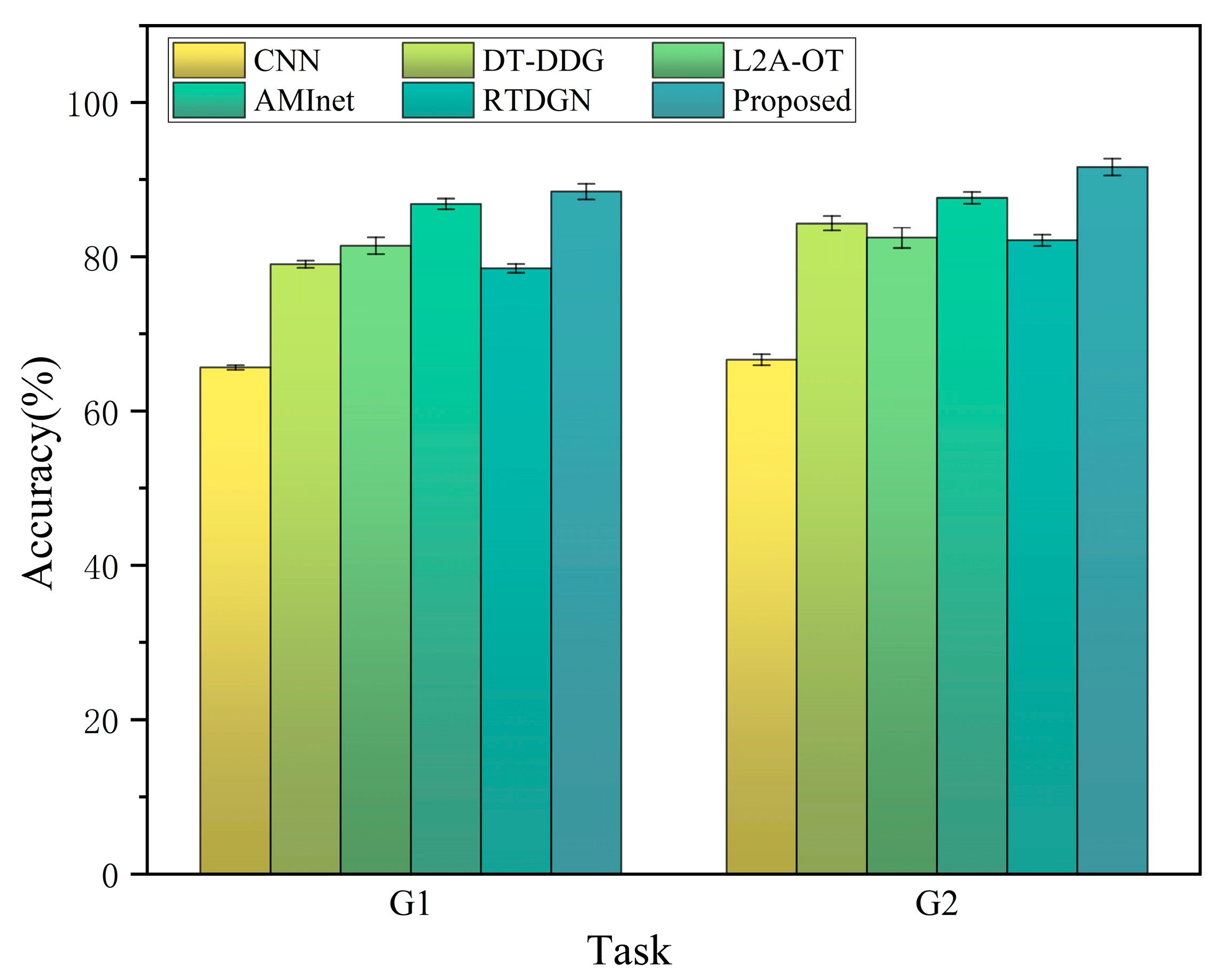
4.2. Comparison Experiment
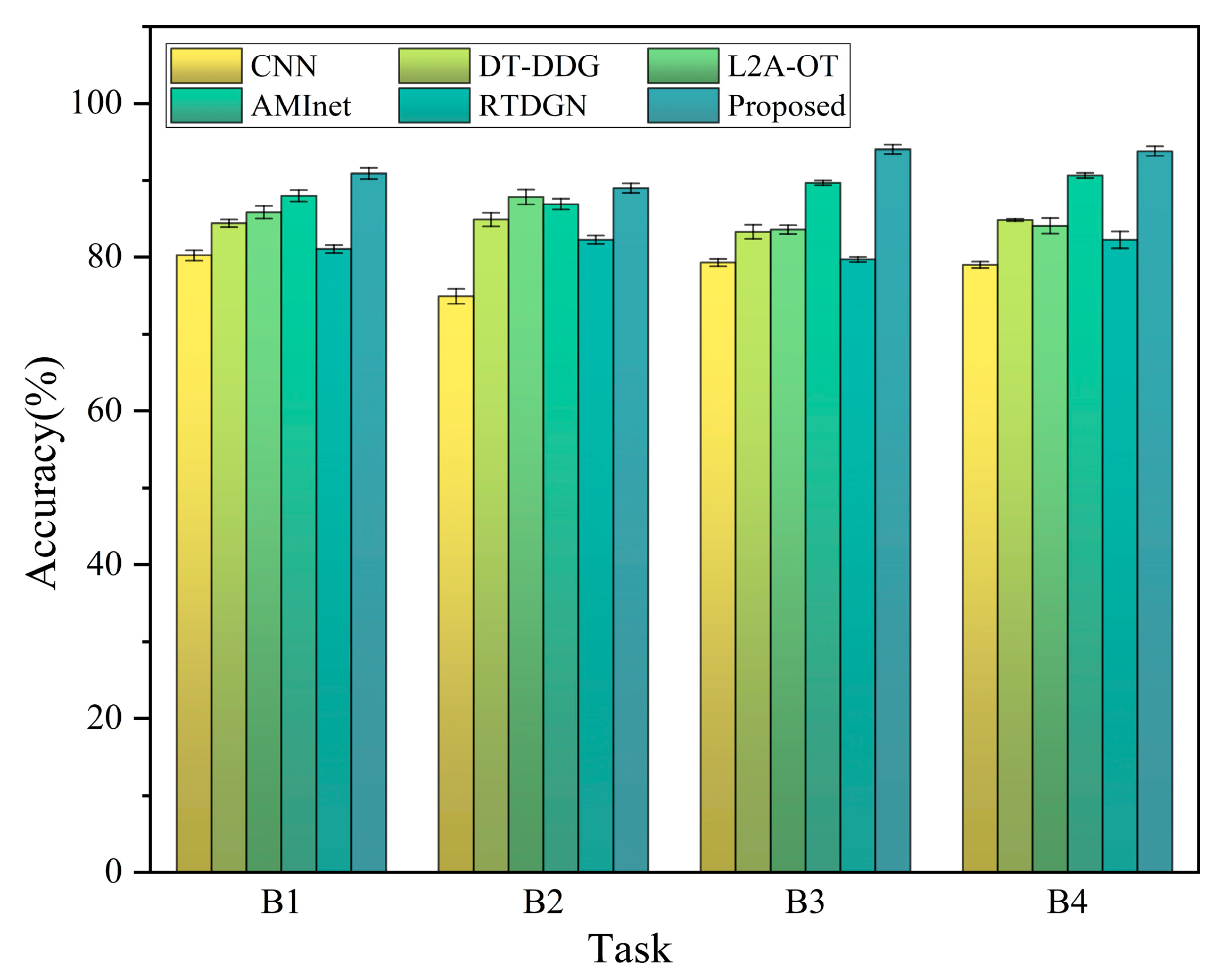
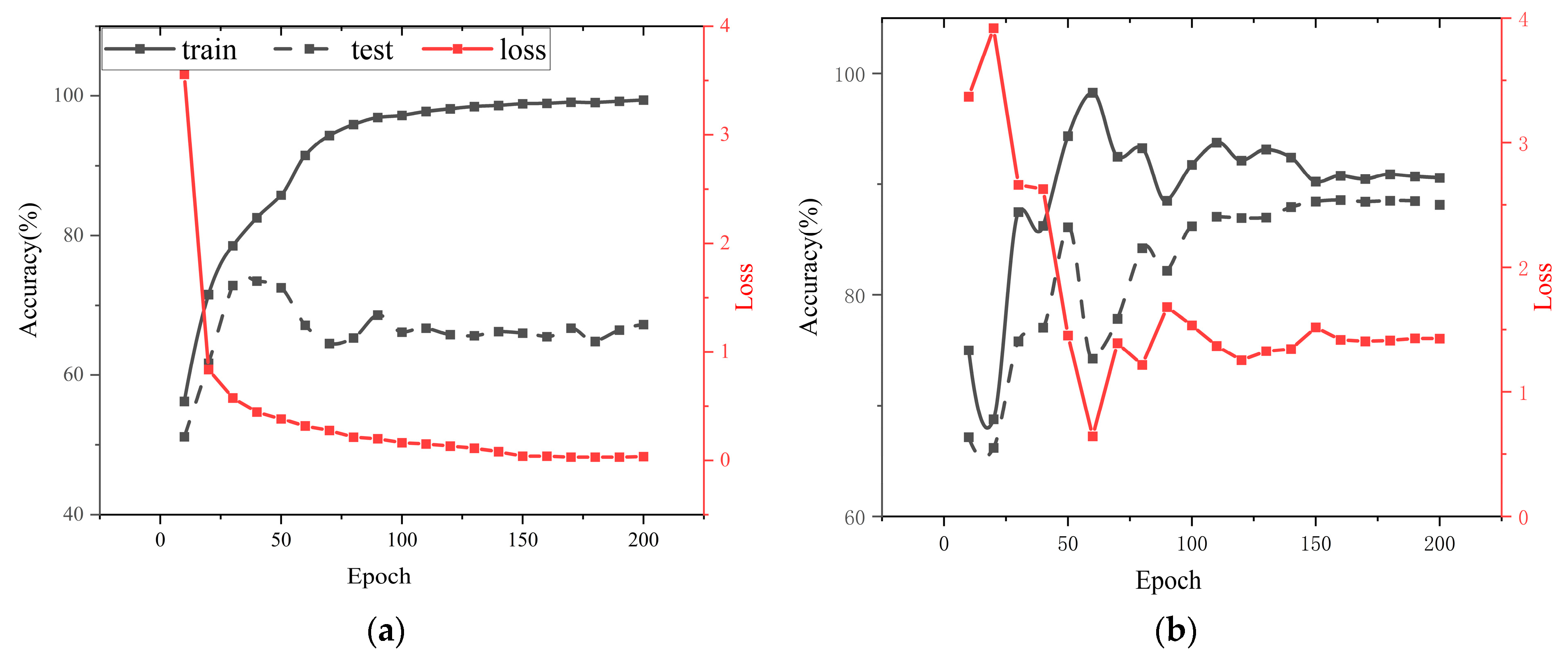
4.3. Experimental Results
4.4. Visualization Analysis
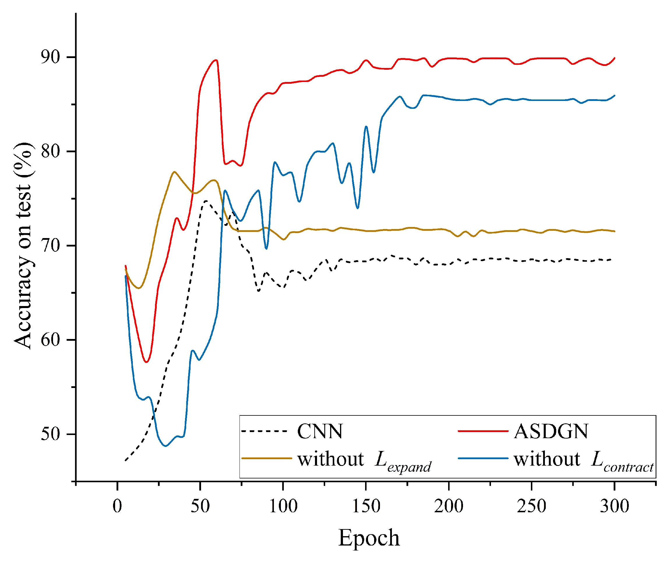
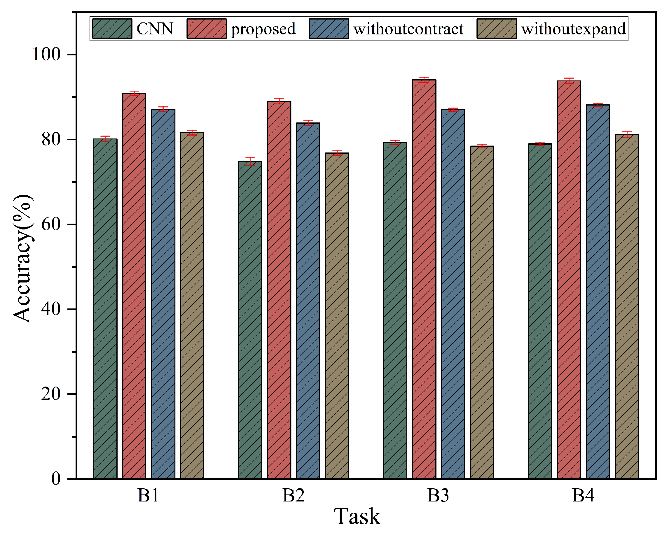
4.5. Ablation Experiments
5. Conclusions
Author Contributions
Funding
Institutional Review Board Statement
Informed Consent Statement
Data Availability Statement
Conflicts of Interest
References
- Zhang, F.H.; Chen, M.S.; Zhu, Y.Z.; Zhang, K.; Li, Q.A. A Review of Fault Diagnosis, Status Prediction, and Evaluation Technology for Wind Turbines. Energies 2023, 16, 1125. [Google Scholar] [CrossRef]
- Liu, Z.P.; Zhang, L. A review of failure modes, condition monitoring and fault diagnosis methods for large-scale wind turbine bearings. Measurement 2020, 149, 22. [Google Scholar] [CrossRef]
- Nguyen, C.D.; Prosvirin, A.; Kim, J.M. A reliable fault diagnosis method for a gearbox system with varying rotational speeds. Sensors 2020, 20, 3105. [Google Scholar] [CrossRef] [PubMed]
- Saucedo-Dorantes, J.J.; Delgado-Prieto, M.; Osornio-Rios, R.A.; Romero-Troncoso, R.D.J. Diagnosis methodology for identifying gearbox wear based on statistical time feature reduction. Proc. Inst. Mech. Eng. Part C J. Mech. Eng. Sci. 2018, 232, 2711–2722. [Google Scholar] [CrossRef]
- Zhang, K.; Tang, B.; Qin, Y.; Deng, L. Fault diagnosis of planetary gearbox using a novel semi-supervised method of multiple association layers networks. Mech. Syst. Signal Process. 2019, 131, 243–260. [Google Scholar] [CrossRef]
- Hu, R.H.; Zhang, M.; Xiang, Z.Y.; Mo, J.L. Guided deep subdomain adaptation network for fault diagnosis of different types of rolling bearings. J. Intell. Manuf. 2023, 34, 2225–2240. [Google Scholar] [CrossRef]
- Wu, H.; Li, J.M.; Zhang, Q.Y.; Tao, J.X.; Meng, Z. Intelligent fault diagnosis of rolling bearings under varying operating conditions based on domain-adversarial neural network and attention mechanism. ISA Trans. 2022, 130, 477–489. [Google Scholar] [CrossRef]
- Wang, Q.B.; Xu, Y.B.; Yang, S.K.; Chang, J.T.; Zhang, J.G.; Kong, X.G. A domain adaptation method for bearing fault diagnosis using multiple incomplete source data. J. Intell. Manuf. 2023, 1–15. [Google Scholar] [CrossRef]
- Zhang, S.Y.; Su, L.; Gu, J.F.; Li, K.; Zhou, L.; Pecht, M. Rotating machinery fault detection and diagnosis based on deep domain adaptation: A survey. Chin. J. Aeronaut. 2023, 36, 45–74. [Google Scholar] [CrossRef]
- Tian, M.; Su, X.M.; Chen, C.Z.; Luo, Y.Q.; Sun, X.M. Bearing fault diagnosis of wind turbines based on dynamic multi-adversarial adaptive network. J. Mech. Sci. Technol. 2023, 37, 1637–1651. [Google Scholar] [CrossRef]
- Li, D.D.; Zhao, Y.; Zhao, Y. A dynamic-model-based fault diagnosis method for a wind turbine planetary gearbox using a deep learning network. Prot. Control Mod. Power Syst. 2022, 7, 14. [Google Scholar] [CrossRef]
- Zhao, K.; Jia, F.; Shao, H.D. A novel conditional weighting transfer Wasserstein auto-encoder for rolling bearing fault diagnosis with multi-source domains. Knowl. Based Syst. 2023, 262, 11. [Google Scholar] [CrossRef]
- Shen, Y.J.; Chen, B.; Guo, F.H.; Meng, W.C.; Yu, L. A Modified Deep Convolutional Subdomain Adaptive Network Method for Fault Diagnosis of Wind Turbine Systems. IEEE Trans. Instrum. Meas. 2022, 71, 10. [Google Scholar] [CrossRef]
- Zhao, C.; Shen, W.M. Mutual-assistance semisupervised domain generalization network for intelligent fault diagnosis under unseen working conditions. Mech. Syst. Signal Proc. 2023, 189, 18. [Google Scholar] [CrossRef]
- Jiang, K.X.; Gao, X.J.; Gao, H.H.; Han, H.Y.; Qi, Y.S. VIT-GADG: A Generative Domain-Generalized Framework for Chillers Fault Diagnosis Under Unseen Working Conditions. IEEE Trans. Instrum. Meas. 2023, 72, 13. [Google Scholar] [CrossRef]
- Qiu, G.Q.; Gu, Y.K.; Cai, Q. A deep convolutional neural networks model for intelligent fault diagnosis of a gearbox under different operational conditions. Measurement 2019, 145, 94–107. [Google Scholar] [CrossRef]
- Durbhaka, G.K.; Selvaraj, B.; Mittal, M.; Saba, T.; Rehman, A.; Goyal, L.M. Swarm-LSTM: Condition Monitoring of Gearbox Fault Diagnosis Based on Hybrid LSTM Deep Neural Network Optimized by Swarm Intelligence Algorithms. CMC-Comput. Mat. Contin. 2021, 66, 2041–2059. [Google Scholar]
- Wang, F.T.; Dun, B.S.; Liu, X.F.; Xue, Y.H.; Li, H.K.; Han, Q.K. An Enhancement Deep Feature Extraction Method for Bearing Fault Diagnosis Based on Kernel Function and Autoencoder. Shock Vib. 2018, 2018, 12. [Google Scholar] [CrossRef]
- Guo, L.; Lei, Y.G.; Xing, S.B.; Yan, T.; Li, N.P. Deep Convolutional Transfer Learning Network: A New Method for Intelligent Fault Diagnosis of Machines with Unlabeled Data. IEEE Trans. Ind. Electron. 2019, 66, 7316–7325. [Google Scholar] [CrossRef]
- Wan, L.J.; Li, Y.Y.; Chen, K.Y.; Gong, K.; Li, C.Y. A novel deep convolution multi-adversarial domain adaptation model for rolling bearing fault diagnosis. Measurement 2022, 191, 17. [Google Scholar] [CrossRef]
- Chen, Z.Y.; He, G.L.; Li, J.P.; Liao, Y.X.; Gryllias, K.; Li, W.H. Domain Adversarial Transfer Network for Cross-Domain Fault Diagnosis of Rotary Machinery. IEEE Trans. Instrum. Meas. 2020, 69, 8702–8712. [Google Scholar] [CrossRef]
- An, Y.Y.; Zhang, K.; Chai, Y.; Liu, Q.; Huang, X.H. Domain adaptation network base on contrastive learning for bearings fault diagnosis under variable working conditions. Expert Syst. Appl. 2023, 212, 9. [Google Scholar] [CrossRef]
- Han, T.; Li, Y.F.; Qian, M. A Hybrid Generalization Network for Intelligent Fault Diagnosis of Rotating Machinery Under Unseen Working Conditions. IEEE Trans. Instrum. Meas. 2021, 70, 11. [Google Scholar] [CrossRef]
- Shi, Y.W.; Deng, A.D.; Deng, M.Q.; Xu, M.; Liu, Y.; Ding, X.; Bian, W.B. Domain augmentation generalization network for real-time fault diagnosis under unseen working conditions. Reliab. Eng. Syst. Saf. 2023, 235, 109188. [Google Scholar] [CrossRef]
- Fan, Z.H.; Xu, Q.F.; Jiang, C.X.; Ding, S.X. Deep Mixed Domain Generalization Network for Intelligent Fault Diagnosis Under Unseen Conditions. IEEE Trans. Ind. Electron. 2023, 71, 965–974. [Google Scholar] [CrossRef]
- Sagawa, S.; Koh, P.W.; Hashimoto, T.B.; Liang, P. Distributionally robust neural networks for group shifts: On the importance of regularization for worst-case generalization. arXiv 2019, arXiv:1911.08731. [Google Scholar]
- Zhang, M.; Marklund, H.; Dhawan, N.; Gupta, A.; Levine, S.; Finn, C. Adaptive Risk Minimization: Learning to Adapt to Domain Shift. In Proceedings of the 35th Conference on Neural Information Processing Systems (NeurIPS), Online, 6–14 December 2021; Neural Information Processing Systems Foundation, Inc. (NeurIPS): Montreal, QC, Canada, 2021. [Google Scholar]
- Balaji, Y.; Sankaranarayanan, S.; Chellappa, R. MetaReg: Towards Domain Generalization using Meta-Regularization. In Proceedings of the 32nd Conference on Neural Information Processing Systems (NIPS), Montreal, QC, Canada, 2–8 December 2018; Neural Information Processing Systems (Nips): Montreal, QC, Canada, 2018. [Google Scholar]
- Qiao, F.; Zhao, L.; Peng, X. Learning to learn single domain generalization. In Proceedings of the IEEE/CVF Conference on Computer Vision and Pattern Recognition, Seattle, WA, USA, 13–19 June 2020; pp. 12556–12565. [Google Scholar]
- Muandet, K.; Balduzzi, D.; Schölkopf, B. Domain generalization via invariant feature representation. In Proceedings of the 30th International Conference on Machine Learning, Atlanta, GA, USA, 17–19 June 2013; pp. 10–18. [Google Scholar]
- Li, H.; Pan, S.J.; Wang, S.; Kot, A.C. Domain generalization with adversarial feature learning. In Proceedings of the IEEE Conference on Computer Vision and Pattern Recognition, Salt Lake City, UT, USA, 18–22 June 2018; pp. 5400–5409. [Google Scholar]
- Mirza, M.; Osindero, S. Conditional generative adversarial nets. arXiv 2014, arXiv:1411.1784. [Google Scholar]
- Ganin, Y.; Ustinova, E.; Ajakan, H.; Germain, P.; Larochelle, H.; Laviolette, F.; Marchand, M.; Lempitsky, V.J.T. Domain-adversarial training of neural networks. J. Mach. Learn. Res. 2016, 17, 1–35. [Google Scholar]
- Kingma, D.P.; Welling, M.J. Auto-encoding variational bayes. arXiv 2013, arXiv:1312.6114. [Google Scholar]
- Pang, X.; Xue, X.; Jiang, W.; Lu, K. An investigation into fault diagnosis of planetary gearboxes using a bispectrum convolutional neural network. IEEE/ASME Trans. Mechatron. 2020, 26, 2027–2037. [Google Scholar] [CrossRef]
- He, C.; Ge, D.; Yang, M.; Yong, N.; Wang, J.; Yu, J.J. A data-driven adaptive fault diagnosis methodology for nuclear power systems based on NSGAII-CNN. Ann. Nucl. Energy 2021, 159, 108326. [Google Scholar] [CrossRef]
- Senanayaka, J.S.L.; Van Khang, H.; Robbersmvr, K.G. CNN based Gearbox Fault Diagnosis and Interpretation of Learning Features. In Proceedings of the 30th IEEE International Symposium on Industrial Electronics (ISIE), Kyoto, Japan, 20–23 June 2021. [Google Scholar]
- Song, B.Y.; Liu, Y.Y.; Lu, P.; Bai, X.Z. Rolling Bearing Fault Diagnosis Based on Time-frequency Transform-assisted CNN: A Comparison Study. In Proceedings of the IEEE 12th Data Driven Control and Learning Systems Conference (DDCLS), Xiangtan, China, 12–14 May 2023; pp. 1273–1279. [Google Scholar]
- Zhao, H.; Liu, M.; Sun, Y.; Chen, Z.; Duan, G.; Cao, X.J. Fault diagnosis of control moment gyroscope based on a new CNN scheme using attention-enhanced convolutional block. Sci. China Technol. Sci. 2022, 65, 2605–2616. [Google Scholar] [CrossRef]
- Yan, X.; She, D.; Xu, Y.; Jia, M.J. Deep regularized variational autoencoder for intelligent fault diagnosis of rotor–bearing system within entire life-cycle process. Knowl. Based Syst. 2021, 226, 107142. [Google Scholar] [CrossRef]
- Rathore, M.S.; Harsha, S.J. Technologies, Non-linear Vibration Response Analysis of Rolling Bearing for Data Augmentation and Characterization. J. Vib. Eng. Technol. 2023, 11, 2109–2131. [Google Scholar] [CrossRef]
- Smith, W.A.; Randall, R.B. Rolling element bearing diagnostics using the Case Western Reserve University data: A benchmark study. Mech. Syst. Signal Process. 2015, 64, 100–131. [Google Scholar] [CrossRef]
- Shao, S.; McAleer, S.; Yan, R.; Baldi, P.J. Highly accurate machine fault diagnosis using deep transfer learning. IEEE Trans. Ind. Inform. 2018, 15, 2446–2455. [Google Scholar] [CrossRef]
- Shi, Y.; Deng, A.; Deng, M.; Li, J.; Xu, M.; Zhang, S.; Ding, X.; Xu, S.J. Domain Transferability-based Deep Domain Generalization Method Towards Actual Fault Diagnosis Scenarios. IEEE Trans. Ind. Inform. 2022, 19, 7355–7366. [Google Scholar] [CrossRef]
- Zhou, K.; Yang, Y.; Hospedales, T.; Xiang, T. Learning to generate novel domains for domain generalization. In Computer Vision—ECCV 2020: Proceedings of the 16th European Conference, Glasgow, UK, 23–28 August 2020; Springer: Cham, Switzerland, 2020; pp. 561–578. [Google Scholar]
- Zhao, C.; Shen, W.J. Adversarial mutual information-guided single domain generalization network for intelligent fault diagnosis. IEEE Trans. Ind. Inform. 2022, 19, 2909–2918. [Google Scholar] [CrossRef]
- Qian, Q.; Zhou, J.; Qin, Y.J. Relationship transfer domain generalization network for rotating machinery fault diagnosis under different working conditions. IEEE Trans. Ind. Inform. 2023, 19, 9898–9908. [Google Scholar] [CrossRef]
- She, D.; Chen, J.; Yan, X.; Zhao, X.; Pecht, M.J. Diversity maximization-based transfer diagnosis approach of rotating machinery. Struct. Health Monit. 2023, 23, 14759217231164921. [Google Scholar] [CrossRef]


| Method | Training Conditions | Target Conditions | ||||||
|---|---|---|---|---|---|---|---|---|
| Source Domain Data | Source Domain Labels | Target Domain Data | Target Domain Labels | Multi-Source Domain for Training | Same Distribution between the Source and Target Domains | Different Distribution between the Source and Target Domains | Multi-Target Domains | |
| DL | ✓ | ✓ | ✕ | ✕ | ✕ | ✓ | ✕ | ✕ |
| DA | ✓ | ✓ | ✓ | ✕ | ✕ | ✓ | ✓ | ✕ |
| DG | ✓ | ✓ | ✕ | ✕ | ✓ | ✓ | ✓ | ✓ |
| SDG | ✓ | ✓ | ✕ | ✕ | ✕ | ✓ | ✓ | ✓ |
| Task | Train Data | Text Data | ||
|---|---|---|---|---|
| Condition | Number | Condition | Number | |
| B1 | 0 (Nm) | 1000 × 4 = 4000 | 0 Nm, 2 Nm, 4 Nm, 8 Nm | 300 × 4 × 4 = 4800 |
| B2 | 2 (Nm) | 1000 × 4 = 4000 | ||
| B3 | 4 (Nm) | 1000 × 4 = 4000 | ||
| B4 | 8 (Nm) | 1000 × 4 = 4000 | ||
| G1 | 20–0 (rpm-V) | 1000 × 5 = 5000 | 20 rpm–0 V, 30 rpm–2 V | 300 × 5 × 2 = 3000 |
| G2 | 30–2 (rpm-V) | 1000 × 5 = 5000 | ||
| Method | CNN | DT-DDG | L2A-OT | AMInet | RTDGN | Proposed |
|---|---|---|---|---|---|---|
| B1 | 80.25 ± 0.71 | 84.42 ± 0.49 | 85.84 ± 0.82 | 88.02 ± 0.73 | 81.10 ± 0.51 | 90.90 ± 0.73 |
| B2 | 74.94 ± 0.96 | 84.91 ± 0.87 | 87.85 ± 0.95 | 86.91 ± 0.71 | 82.29 ± 0.55 | 88.99 ± 0.62 |
| B3 | 79.28 ± 0.49 | 83.32 ± 0.91 | 83.61 ± 0.57 | 89.69 ± 0.32 | 79.70 ± 0.33 | 94.07 ± 0.59 |
| B4 | 79.00 ± 0.43 | 84.83 ± 0.16 | 84.08 ± 1.00 | 90.64 ± 0.32 | 82.29 ± 1.08 | 93.83 ± 0.63 |
| Average | 78.37 | 84.37 | 85.35 | 88.82 | 81.35 | 91.95 |
| Method | CNN | DT-DDG | L2A-OT | AMInet | RTDGN | Proposed |
|---|---|---|---|---|---|---|
| G1 | 65.66 ± 0.29 | 79.06 ± 0.46 | 81.42 ± 1.07 | 86.86 ± 0.70 | 78.51 ± 0.56 | 88.43 ± 1.01 |
| G2 | 66.67 ± 0.72 | 84.35 ± 0.95 | 82.46 ± 1.31 | 87.63 ± 0.74 | 82.11 ± 0.74 | 91.65 ± 1.08 |
| Average | 66.17 | 81.71 | 81.94 | 87.25 | 80.31 | 90.04 |
| Model | Training Time (s) |
|---|---|
| CNN | 219.37 |
| DT-DDG | 311.54 |
| L2A-OT | 392.78 |
| AMInet | 413.49 |
| RTDGN | 288.15 |
| Proposed | 506.42 |
Disclaimer/Publisher’s Note: The statements, opinions and data contained in all publications are solely those of the individual author(s) and contributor(s) and not of MDPI and/or the editor(s). MDPI and/or the editor(s) disclaim responsibility for any injury to people or property resulting from any ideas, methods, instructions or products referred to in the content. |
© 2023 by the authors. Licensee MDPI, Basel, Switzerland. This article is an open access article distributed under the terms and conditions of the Creative Commons Attribution (CC BY) license (https://creativecommons.org/licenses/by/4.0/).
Share and Cite
Wang, X.; Wang, C.; Liu, H.; Zhang, C.; Fu, Z.; Ding, L.; Bai, C.; Zhang, H.; Wei, Y. An Adversarial Single-Domain Generalization Network for Fault Diagnosis of Wind Turbine Gearboxes. J. Mar. Sci. Eng. 2023, 11, 2384. https://doi.org/10.3390/jmse11122384
Wang X, Wang C, Liu H, Zhang C, Fu Z, Ding L, Bai C, Zhang H, Wei Y. An Adversarial Single-Domain Generalization Network for Fault Diagnosis of Wind Turbine Gearboxes. Journal of Marine Science and Engineering. 2023; 11(12):2384. https://doi.org/10.3390/jmse11122384
Chicago/Turabian StyleWang, Xinran, Chenyong Wang, Hanlin Liu, Cunyou Zhang, Zhenqiang Fu, Lin Ding, Chenzhao Bai, Hongpeng Zhang, and Yi Wei. 2023. "An Adversarial Single-Domain Generalization Network for Fault Diagnosis of Wind Turbine Gearboxes" Journal of Marine Science and Engineering 11, no. 12: 2384. https://doi.org/10.3390/jmse11122384
APA StyleWang, X., Wang, C., Liu, H., Zhang, C., Fu, Z., Ding, L., Bai, C., Zhang, H., & Wei, Y. (2023). An Adversarial Single-Domain Generalization Network for Fault Diagnosis of Wind Turbine Gearboxes. Journal of Marine Science and Engineering, 11(12), 2384. https://doi.org/10.3390/jmse11122384