
A Trajectory Tracking and Local Path Planning Control Strategy for Unmanned Underwater Vehicles


Abstract
:1. Introduction
- A trajectory tracking controller is designed by using the event triggering mechanism and combining the fault state and disturbance state of the UUV actuator, which realizes the classification and collection of the relevant states in the model training and simulation and the seamless connection of the successive tasks.
- Combining the deep reinforcement learning framework with meta-heuristic algorithms in the same task space, the conditions of distance, energy consumption, and steering angle constraints required by UUVs in the task environment are considered from various perspectives, and reward component and angular factors are introduced into the RRT algorithm to locally plan the path.
- In response to the effects of external perturbations and actuator faults, a joint reduced-order extended state observer and feed-forward compensation mechanism is designed to enable the UUV to counteract the unfavorable effects by automatically adjusting its own output.
2. Preliminaries
2.1. Underactuated UUV Model Description
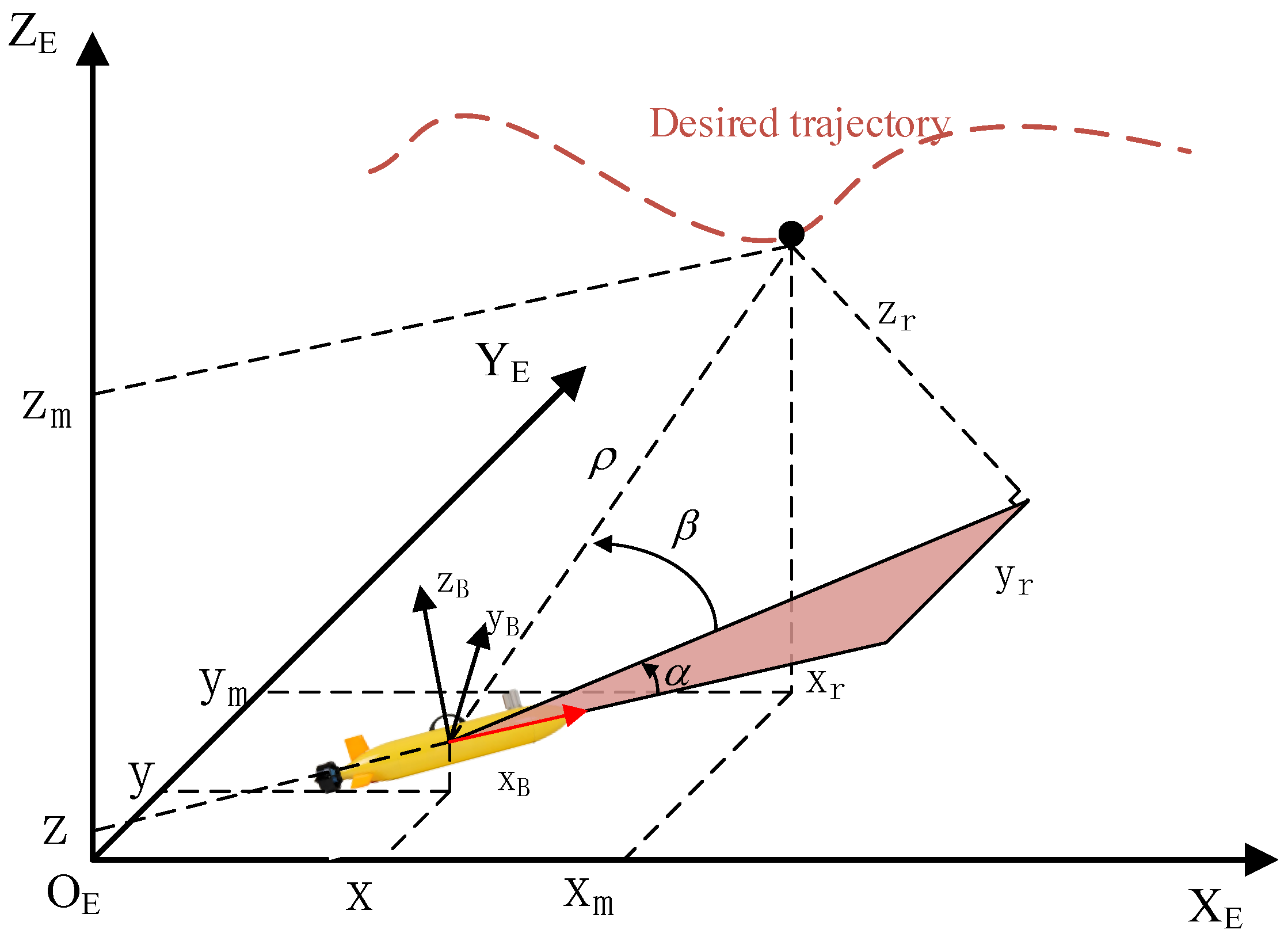
2.2. Tracking the State Model of the Mission Environment
- The motion of the UUV in the roll direction is neglected.
- The UUV has neutral buoyancy, and the origin of the body-fixed coordinates is located at the center of mass.
- The yaw angle is limited to , and the pitch angle is limited to .
- 1.
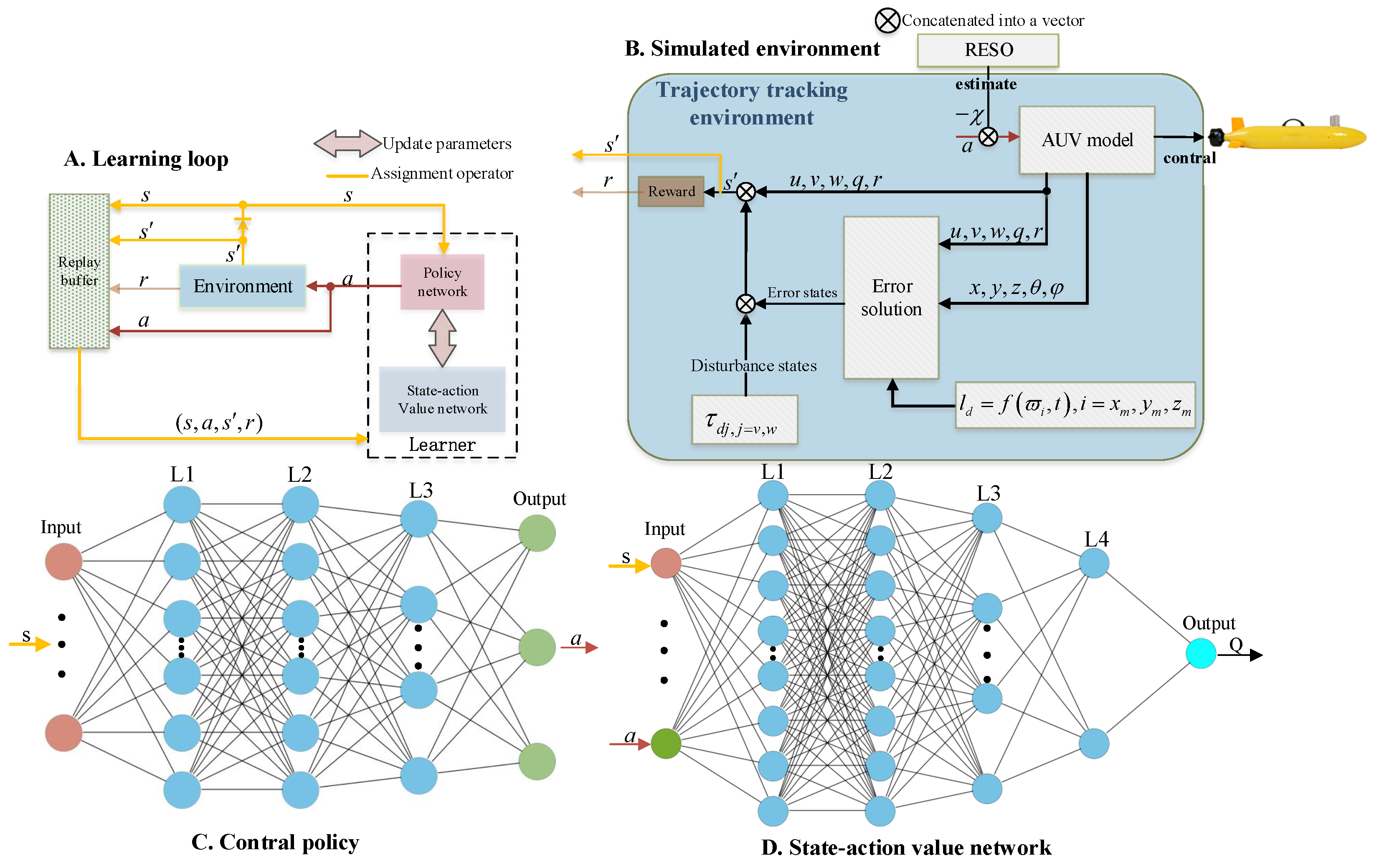
- Trajectory Tracking Task StatusWe selected the velocity state, actuator failure state, and perturbation state, which are directly related to the update of the UUV position, velocity, and acceleration states, as the base states for the policy network inputs. The velocity state can be expressed asSince multiplicative faults are approximated as fixed values, so that they have no effect on the learning update process of the policy network, the fault state should be set as additive faults, denoted as follows:The five-degrees-of-freedom UUV perturbation state can be defined asIn addition, combining the relative distance, relative pitch angle, and relative yaw angle obtained from Equation (4), we set the error state of the trajectory tracking task as follows:where , , and denote the desired relative distance, relative pitch angle, and relative error, respectively.Finally, we can obtain the input state of the trajectory tracking task in the deep reinforcement learning framework:
- 2.
- Action spaceThe UUV studied in this paper is powered by a propeller in the tail and rudders on both sides, with control forces and moments applied to the UUV to update its state over time. Therefore, we directly chose the control force and moment as the output of the deep reinforcement learning strategy network, which can be expressed as
- 3.
- Reward functionThe trajectory tracking task expects the UUV to track the target quickly and maintain a fixed tracking state in a limited time, so the reward function should be selected by first considering the error between the UUV and the desired trajectory, based on the approximation that the larger the error, the smaller the reward. Combining this with Equation (8), one obtainsIn addition, we expect the outputs of the UUV propeller and rudder to be maintained in a more stable and energy-efficient manner, which means that under the condition of achieving the same control accuracy, the smaller the output value, the better the corresponding action. Thus, we define the reward function related to the controller output aswhere and denote the weight parameters of the two-part reward function.
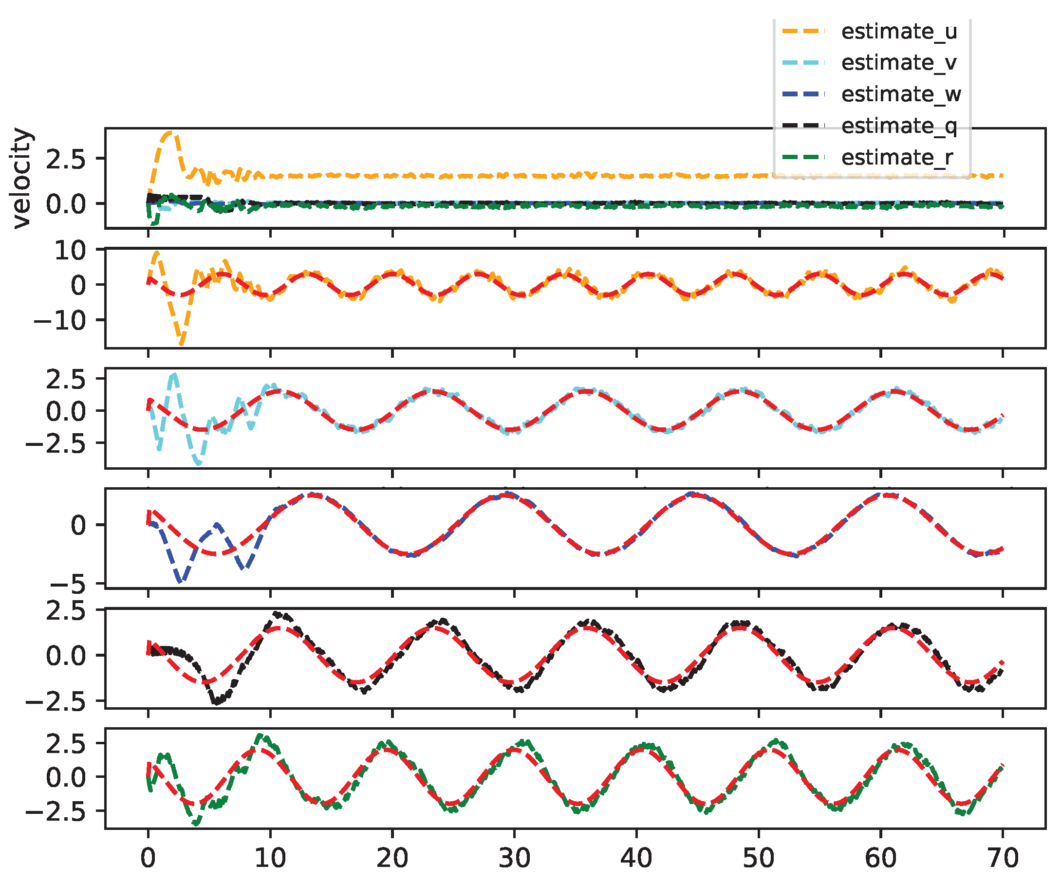
2.3. Reduced-Order Extended State Observer
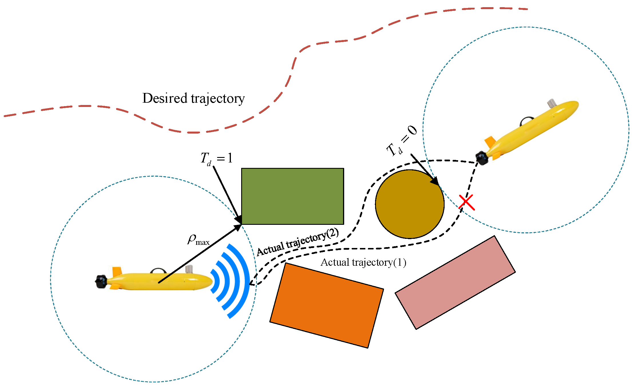
2.4. Localized Planning Mission Environment Model
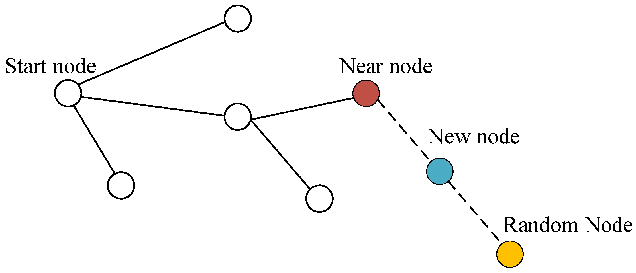
2.5. The Principles of the Basic RRT Algorithm
3. Improved RRT Algorithm with Reinforcement Learning Applications
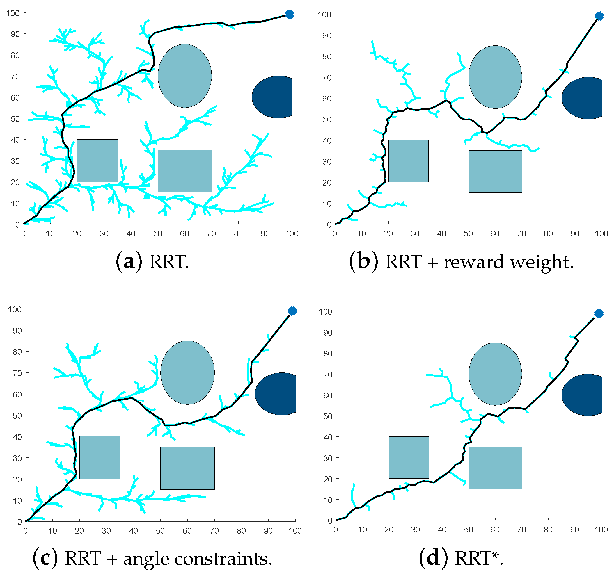
3.1. Improved RRT Algorithm
- 1.
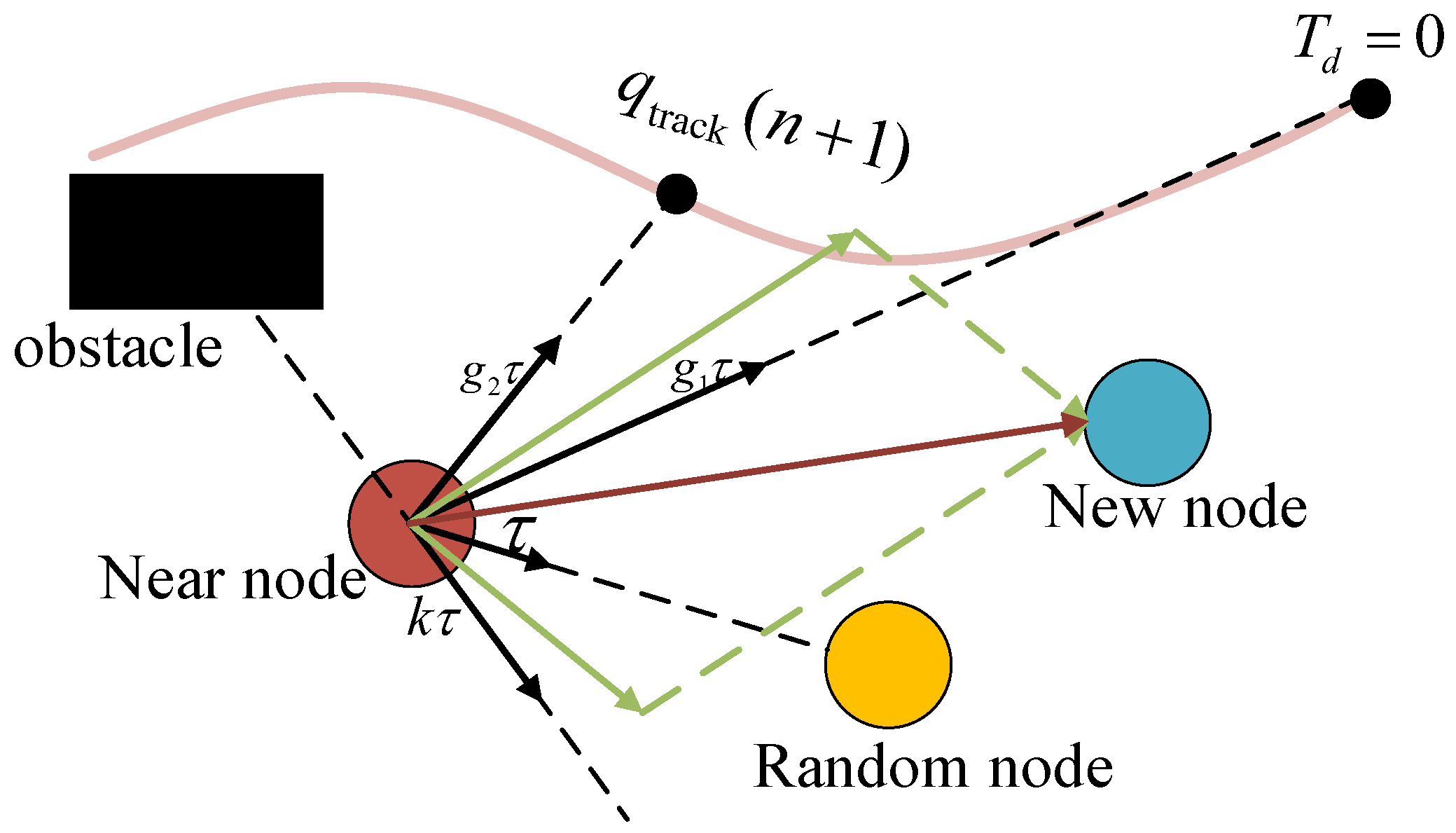
- Rewarding the generation of new nodes that are close to the goal point .According to the basic RRT algorithm, the extension vector of the nearest point can be expressed by the following mathematical formula [21]:where denotes the expansion vector from the nth nearest point to the nth random point , and represents the step size in the RRT algorithm. Then, the reward component from to can be defined aswhere denotes the reward gain coefficient that varies the target bias of the generated random vector.
- 2.
- Rewarding the generation of new nodes that are close to the desired trajectory.The continuous task environment of trajectory tracking and localized obstacle avoidance requires the UUV to complete the switch between the two task states with the smallest possible energy consumption. Therefore, it requires us to keep the error with the desired trajectory small during the planning of the paths. As shown in Figure 3, we plan two actual paths, and only that which is closer to the desired trajectory is selected. Emulating the form of the reward component with respect to , we obtain the reward component with the desired trajectory point of the next time step as the goal:
- 3.
- Rewarding the generation of new nodes that stay away from obstacles.The new node is affected by the reward component introduced between the barrier and as it is generated, which can be expressed as
3.2. Applications of Deep Reinforcement Learning
| Algorithm 1 Pseudo-code of TD3 for UUV path tracking with local path planning |
|
4. Simulation
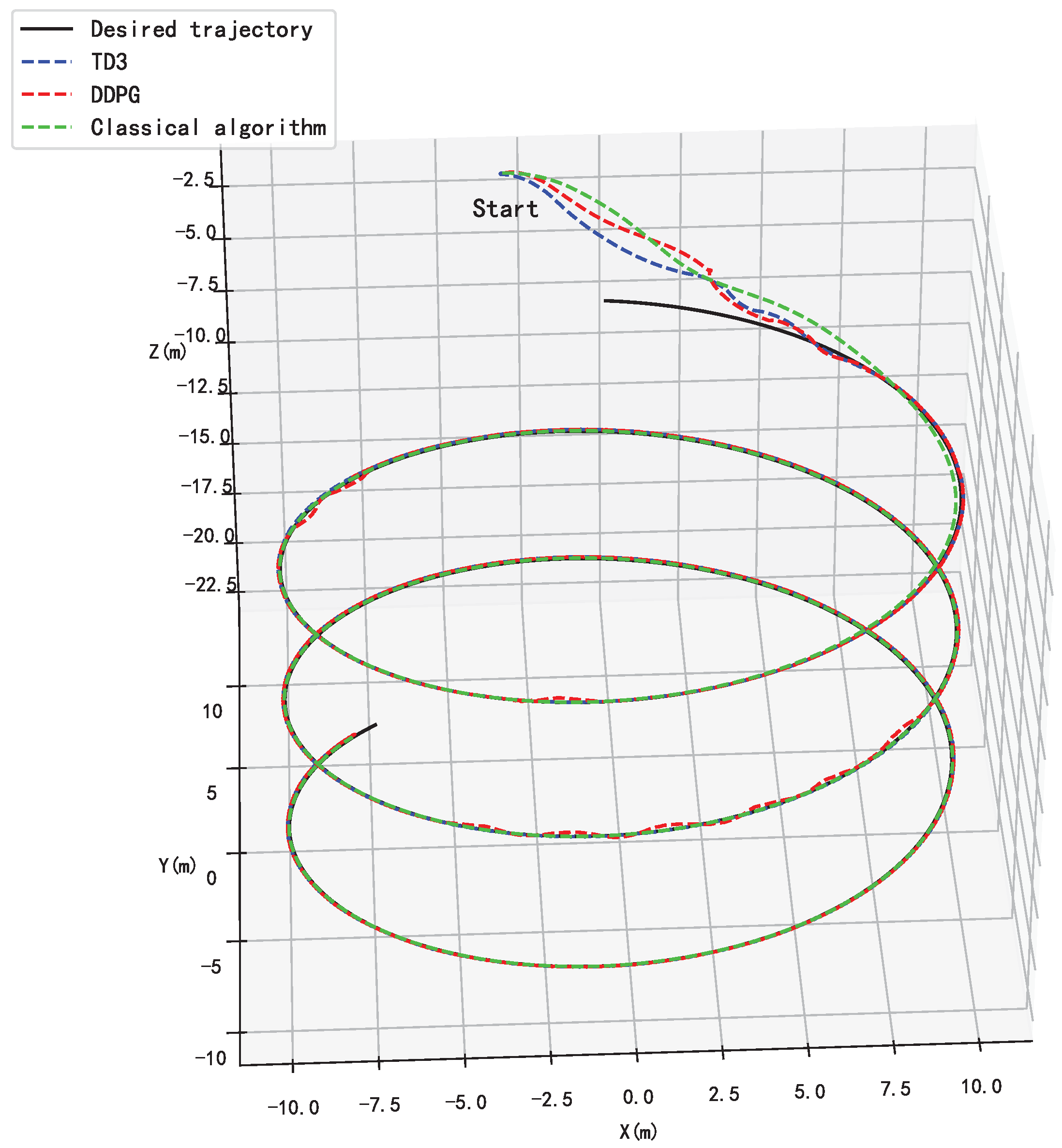
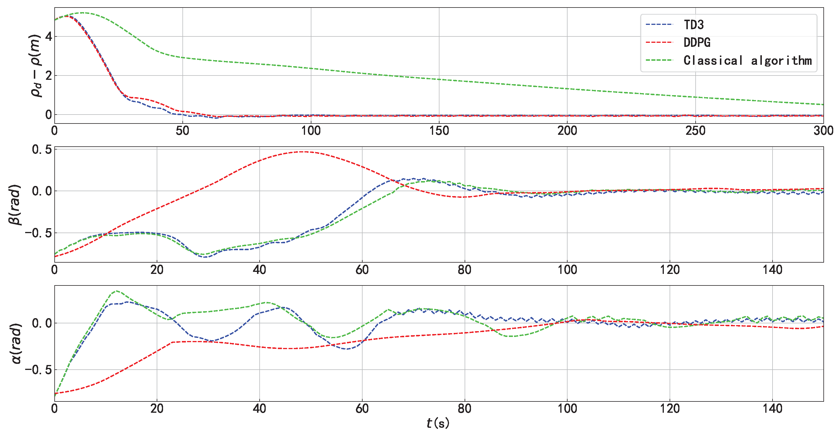
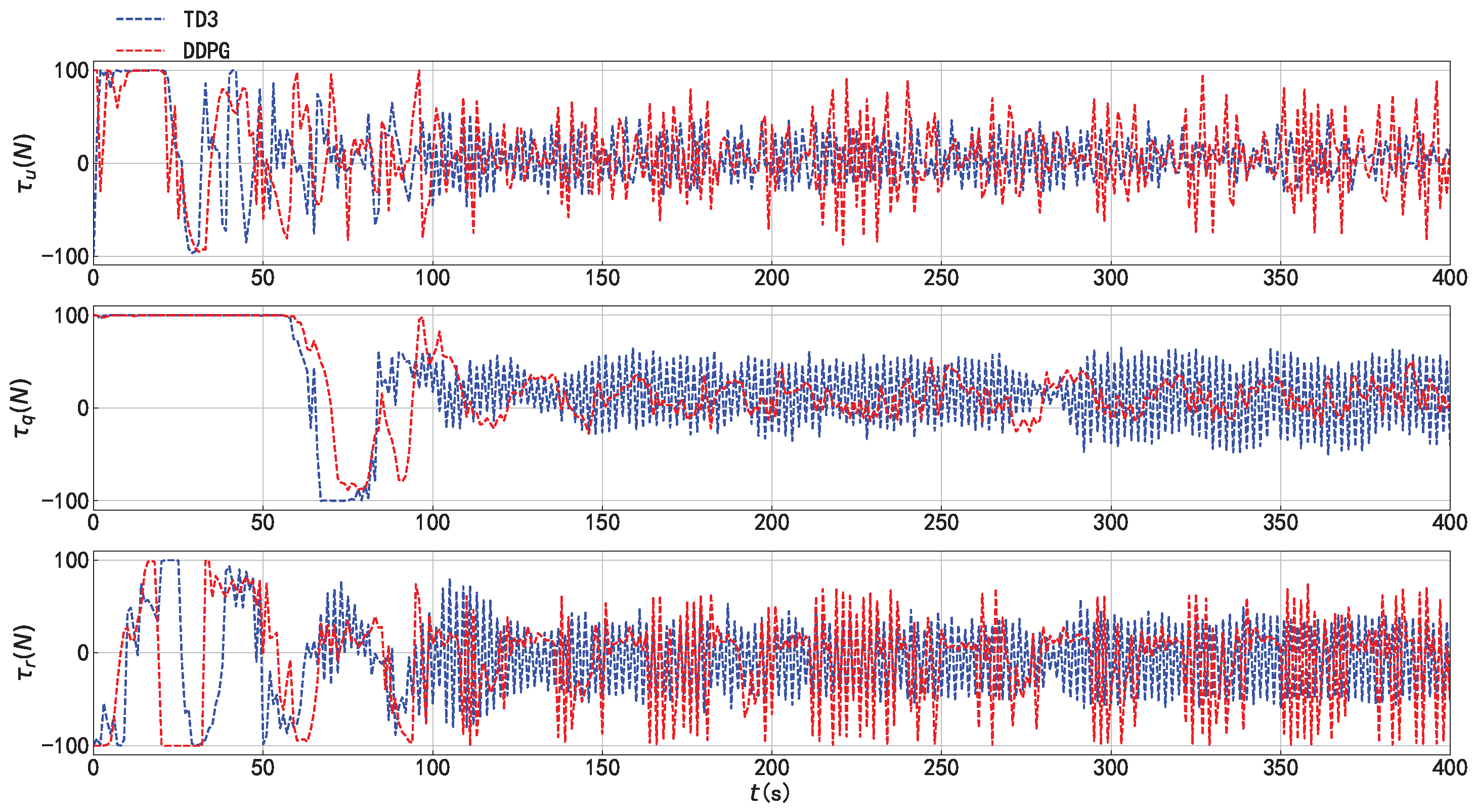
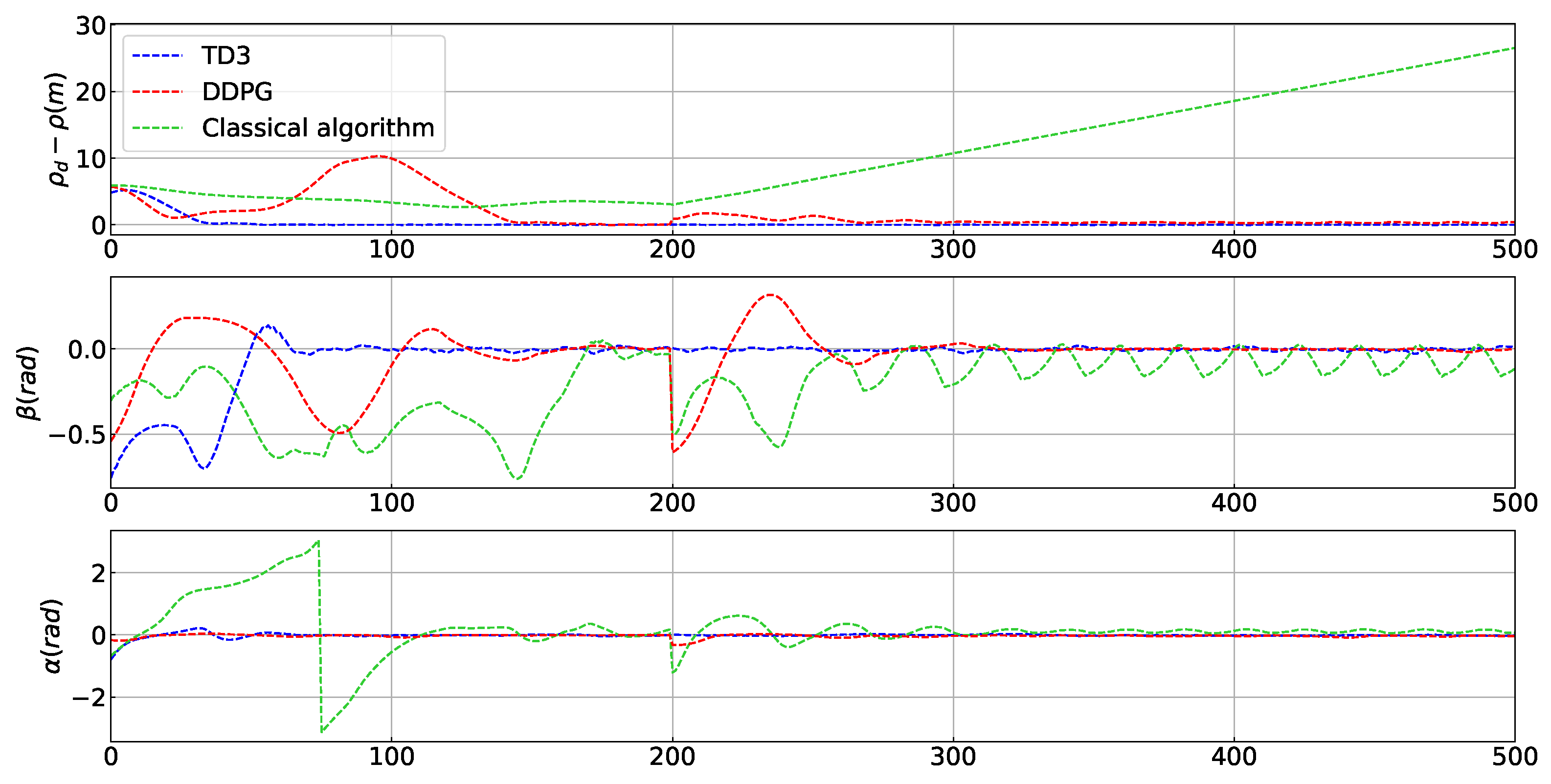
4.1. Trajectory Tracking Capability
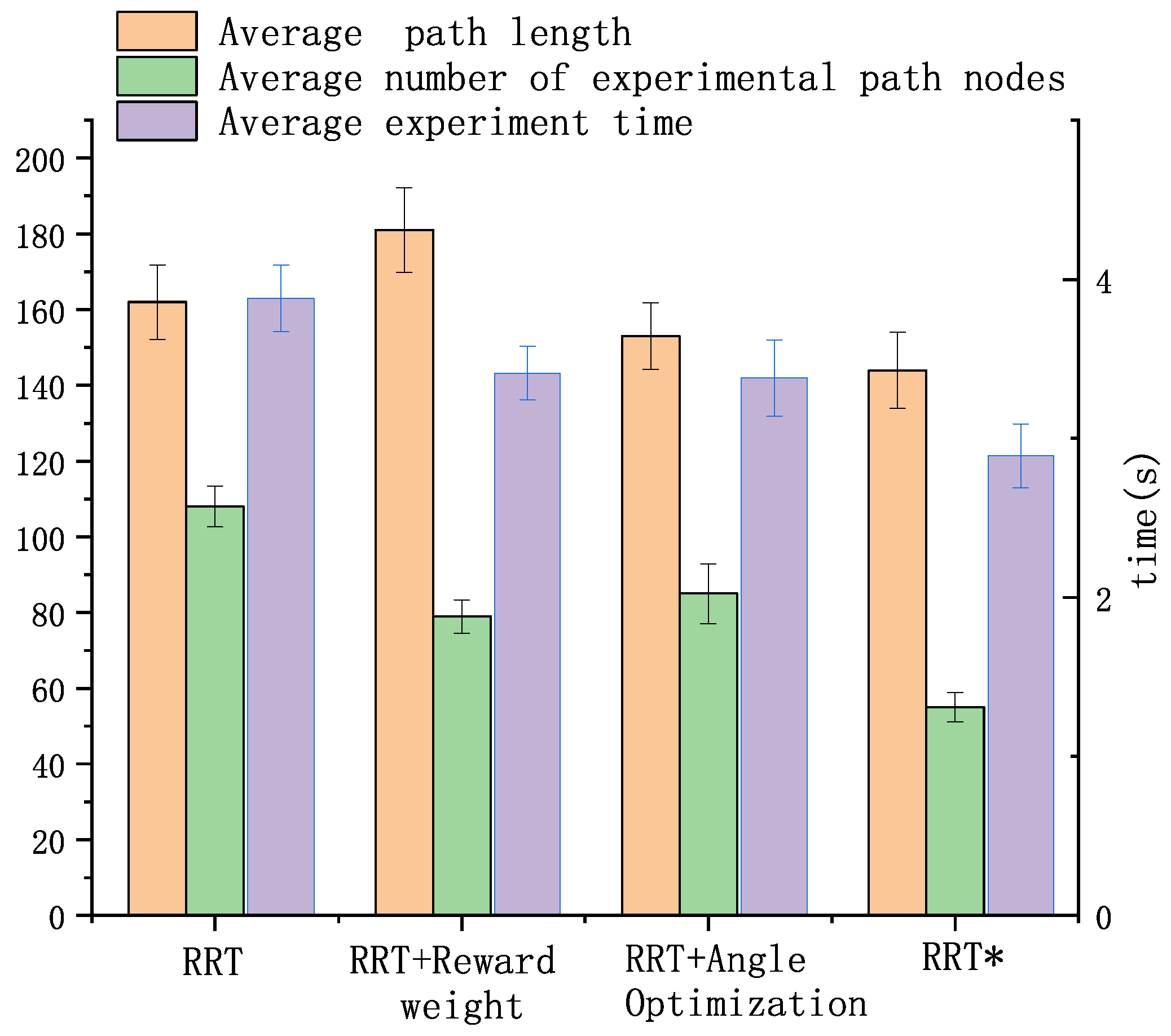
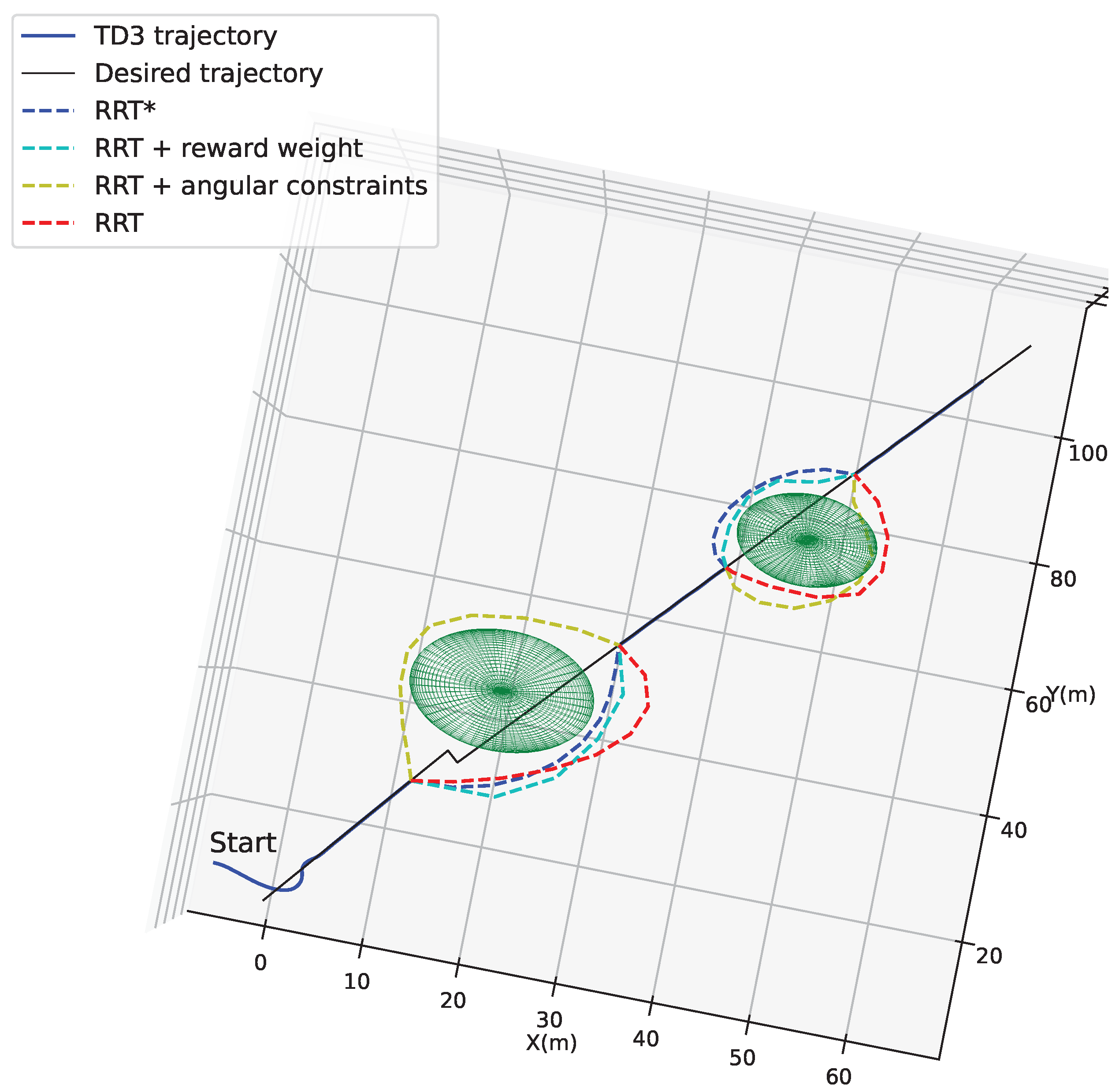
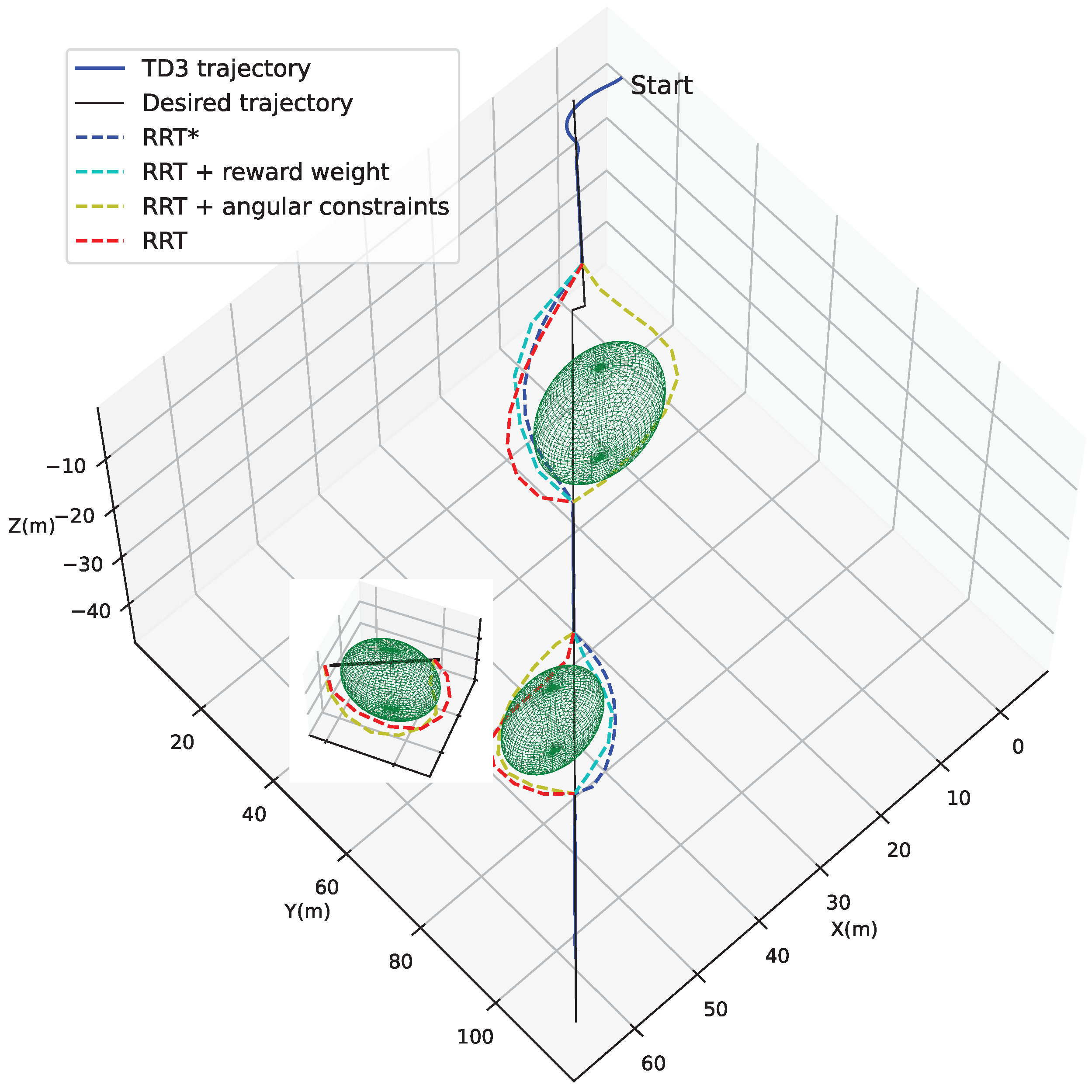
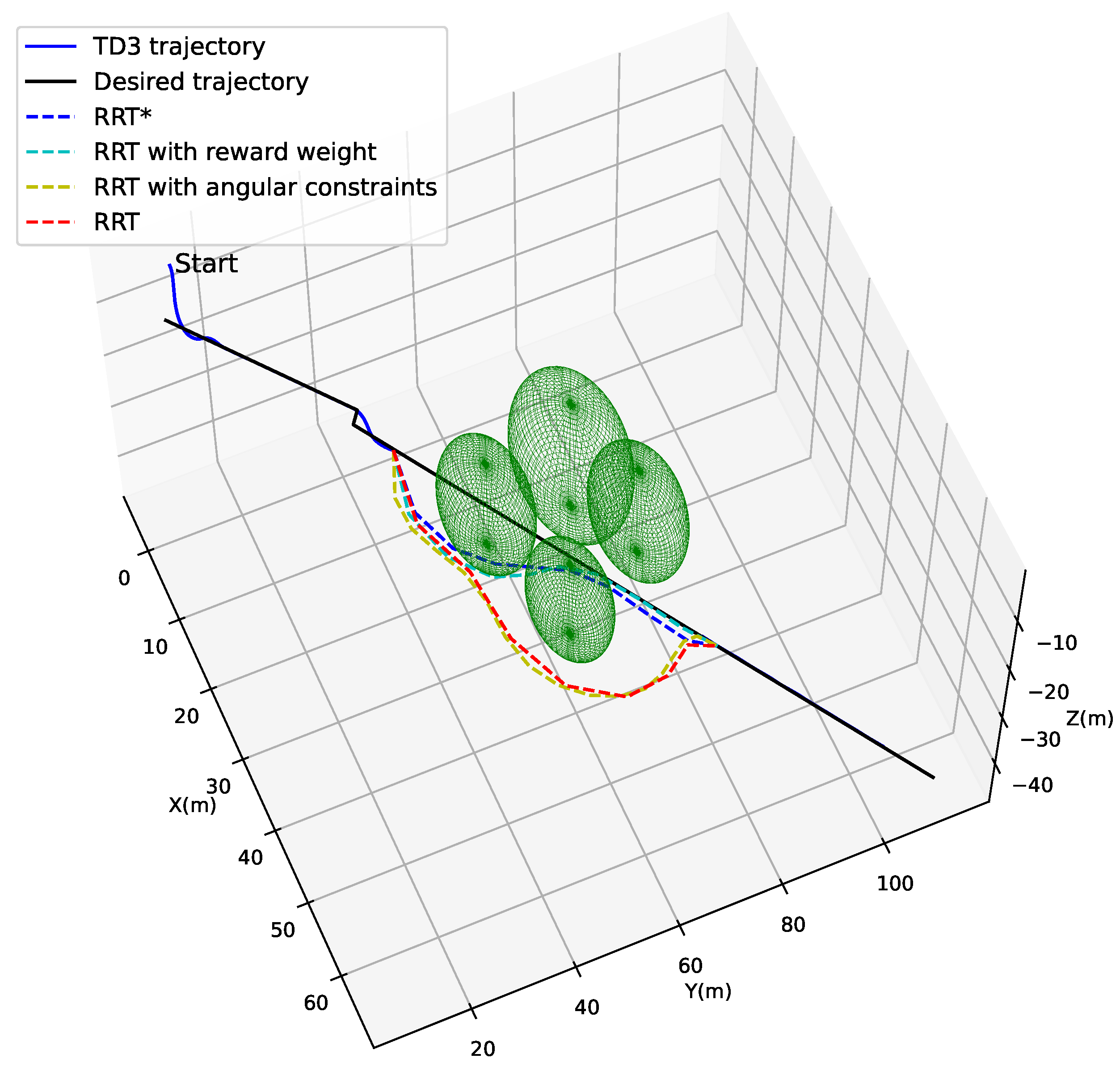
4.2. Localized Path Planning Capability
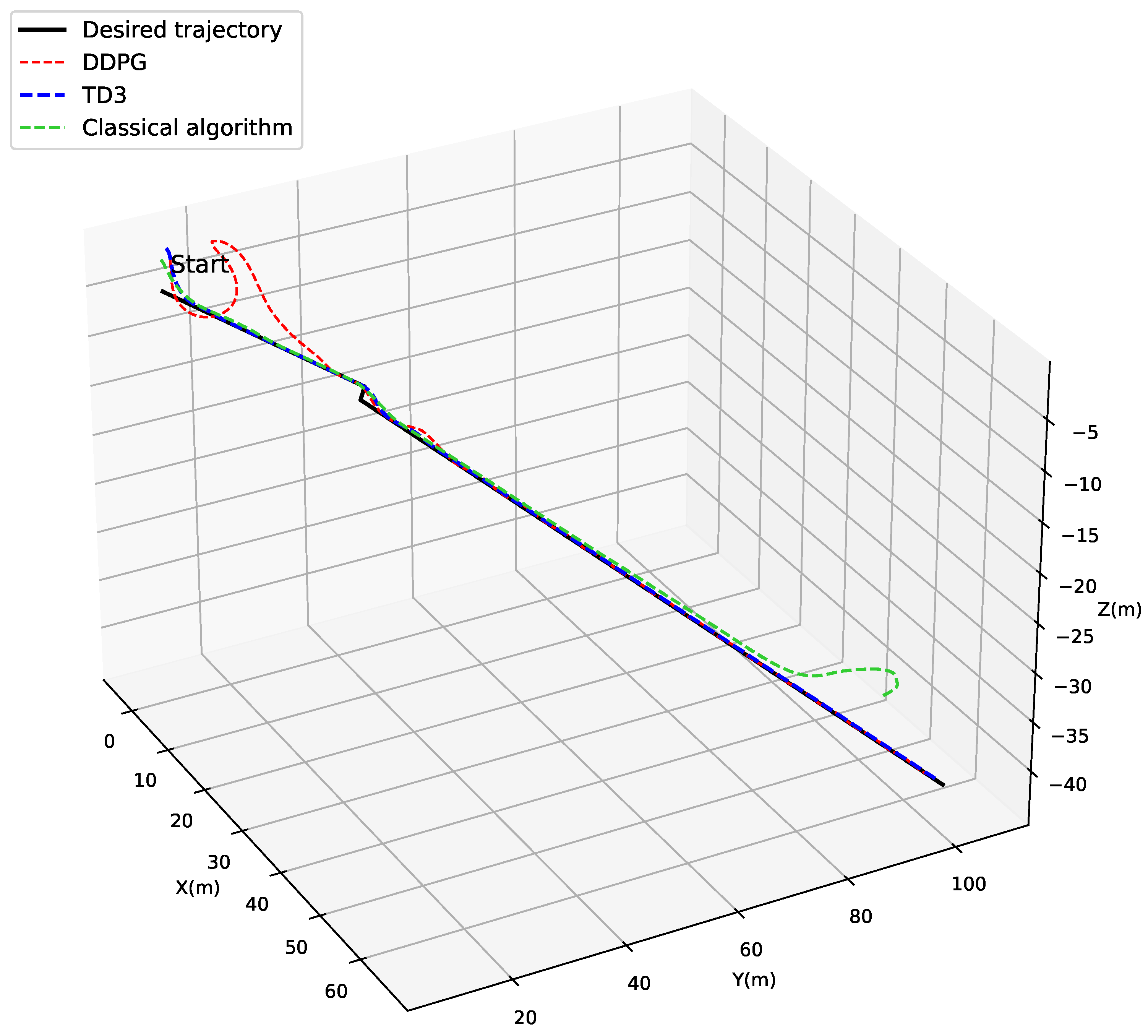
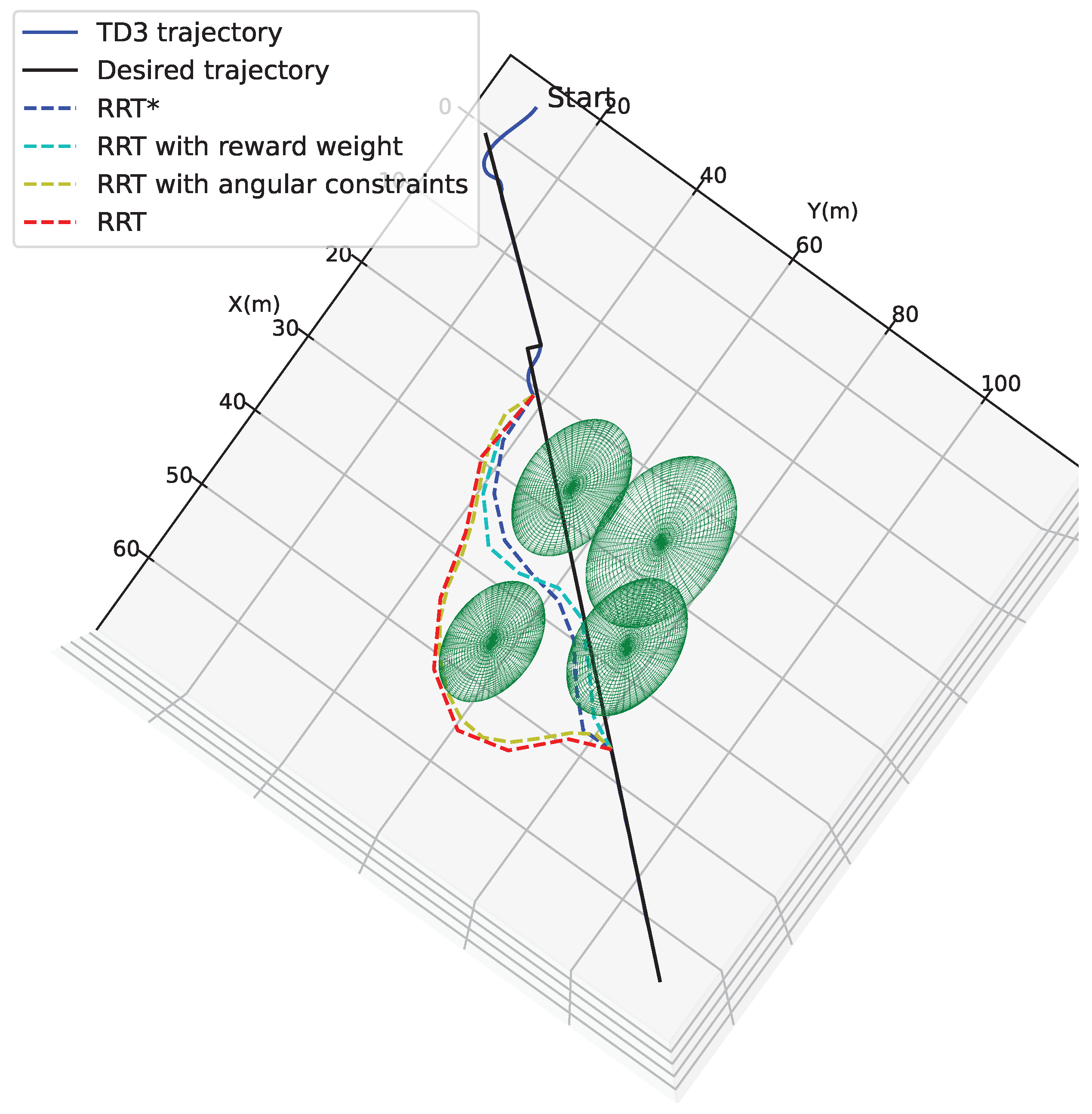
4.3. Trajectory Tracking Combined with Localized Path Planning Capabilities
5. Conclusions
Author Contributions
Funding
Institutional Review Board Statement
Informed Consent Statement
Data Availability Statement
Conflicts of Interest
Appendix A
References
- Zhang, C.; Cheng, P.; Du, B.; Dong, B.; Zhang, W. AUV path tracking with real-time obstacle avoidance via reinforcement learning under adaptive constraints. Ocean Eng. 2022, 256, 111453. [Google Scholar] [CrossRef]
- Lin, X.; Tian, W.; Zhang, W.; Li, Z.; Zhang, C. The fault-tolerant consensus strategy for leaderless Multi-AUV system on heterogeneous condensation topology. Ocean Eng. 2022, 245, 110541. [Google Scholar] [CrossRef]
- Shojaei, K.; Dolatshahi, M. Line-of-sight target tracking control of underactuated autonomous underwater vehicles. Ocean Eng. 2017, 133, 244–252. [Google Scholar] [CrossRef]
- Shen, C.; Shi, Y.; Buckham, B. Trajectory Tracking Control of an Autonomous Underwater Vehicle Using Lyapunov-Based Model Predictive Control. IEEE Trans. Ind. Electron. 2018, 65, 5796–5805. [Google Scholar] [CrossRef]
- Lamraoui, H.C.; Qidan, Z. Path following control of fully-actuated autonomous underwater vehicle in presence of fast-varying disturbances. Appl. Ocean Res. 2019, 86, 40–46. [Google Scholar] [CrossRef]
- Vu, M.T.; Le Thanh, H.N.N.; Huynh, T.T.; Thang, Q.; Duc, T.; Hoang, Q.D.; Le, T.H. Station-keeping control of a hovering over-actuated autonomous underwater vehicle under ocean current effects and model uncertainties in horizontal plane. IEEE Access 2021, 9, 6855–6867. [Google Scholar] [CrossRef]
- Le, T.H.; Thanh, H.L.N.N.; Huynh, T.T.; Van, M.; Hoang, Q.D.; Do, T.D.; Vu, M.T. Robust position control of an over-actuated underwater vehicle under model uncertainties and ocean current effects using dynamic sliding mode surface and optimal allocation control. Sensors 2021, 21, 747. [Google Scholar]
- Yu, C.; Xiang, X.; Wilson, P.A.; Zhang, Q. Guidance-Error-Based Robust Fuzzy Adaptive Control for Bottom Following of a Flight-Style AUV With Saturated Actuator Dynamics. IEEE Trans. Cybern. 2020, 50, 1887–1899. [Google Scholar] [CrossRef]
- Carlucho, I.; De Paula, M.; Wang, S.; Menna, B.V.; Petillot, Y.R.; Acosta, G.G. AUV position tracking control using end-to-end deep reinforcement learning. In Proceedings of the OCEANS 2018 MTS/IEEE Charleston, Charleston, SC, USA, 22–25 October 2018; IEEE: New York, NY, USA, 2018; pp. 1–8. [Google Scholar]
- Mao, Y.; Gao, F.; Zhang, Q.; Yang, Z. An AUV target-tracking method combining imitation learning and deep reinforcement learning. J. Mar. Sci. Eng. 2022, 10, 383. [Google Scholar] [CrossRef]
- Carlucho, I.; De Paula, M.; Wang, S.; Petillot, Y.; Acosta, G.G. Adaptive low-level control of autonomous underwater vehicles using deep reinforcement learning. Robot. Auton. Syst. 2018, 107, 71–86. [Google Scholar] [CrossRef]
- Jiang, J.; Zhang, R.; Fang, Y.; Wang, X. Research on motion attitude control of under-actuated autonomous underwater vehicle based on deep reinforcement learning. J. Phys. Conf. Ser. 2020, 1693, 012206. [Google Scholar] [CrossRef]
- Fang, Y.; Huang, Z.; Pu, J.; Zhang, J. AUV position tracking and trajectory control based on fast-deployed deep reinforcement learning method. Ocean Eng. 2022, 245, 110452. [Google Scholar] [CrossRef]
- Liu, Y.; Wang, F.; Lv, Z.; Cao, K.; Lin, Y. Pixel-to-Action Policy for Underwater Pipeline Following via Deep Reinforcement Learning. In Proceedings of the 2018 IEEE International Conference of Intelligent Robotic and Control Engineering (IRCE), Lanzhou, China, 24–27 August 2018; pp. 135–139. [Google Scholar] [CrossRef]
- Yan, Z.; Yan, J.; Wu, Y.; Cai, S.; Wang, H. A novel reinforcement learning based tuna swarm optimization algorithm for autonomous underwater vehicle path planning. Math. Comput. Simul. 2023, 209, 55–86. [Google Scholar] [CrossRef]
- Zheng, Y.J. Water wave optimization: A new nature-inspired metaheuristic. Comput. Oper. Res. 2015, 55, 1–11. [Google Scholar] [CrossRef]
- Mirjalili, S.; Mirjalili, S.M.; Lewis, A. Grey wolf optimizer. Adv. Eng. Softw. 2014, 69, 46–61. [Google Scholar] [CrossRef]
- Neshat, M.; Sepidnam, G.; Sargolzaei, M.; Toosi, A.N. Artificial fish swarm algorithm: A survey of the state-of-the-art, hybridization, combinatorial and indicative applications. Artif. Intell. Rev. 2014, 42, 965–997. [Google Scholar] [CrossRef]
- Mirjalili, S.; Lewis, A. The whale optimization algorithm. Adv. Eng. Softw. 2016, 95, 51–67. [Google Scholar] [CrossRef]
- Li, J.; Li, C.; Chen, T.; Zhang, Y. Improved RRT algorithm for AUV target search in unknown 3D environment. J. Mar. Sci. Eng. 2022, 10, 826. [Google Scholar] [CrossRef]
- Hong, L.; Song, C.; Yang, P.; Cui, W. Two-Layer Path Planner for AUVs Based on the Improved AAF-RRT Algorithm. J. Mar. Sci. Appl. 2022, 21, 102–115. [Google Scholar] [CrossRef]
- Yu, L.; Wei, Z.; Wang, Z.; Hu, Y.; Wang, H. Path optimization of AUV based on smooth-RRT algorithm. In Proceedings of the 2017 IEEE International Conference on Mechatronics and Automation (ICMA), Kagawa, Japan, 6–9 August 2017; IEEE: New York, NY, USA, 2017; pp. 1498–1502. [Google Scholar]
- Huang, F.; Xu, J.; Wu, D.; Cui, Y.; Yan, Z.; Xing, W.; Zhang, X. A general motion controller based on deep reinforcement learning for an autonomous underwater vehicle with unknown disturbances. Eng. Appl. Artif. Intell. 2023, 117, 105589. [Google Scholar] [CrossRef]
- Fossen, T.I. Handbook of Marine Craft Hydrodynamics and Motion Control; John Wiley & Sons: Hoboken, NJ, USA, 2011. [Google Scholar]
- Xu, J.; Cui, Y.; Yan, Z.; Huang, F.; Du, X.; Wu, D. Event-triggered adaptive target tracking control for an underactuated autonomous underwater vehicle with actuator faults. J. Frankl. Inst. 2023, 360, 2867–2892. [Google Scholar] [CrossRef]
- Tian, G. Reduced-Order Extended State Observer and Frequency Response Analysis. Master’s Thesis, Cleveland State University, Cleveland, OH, USA, 2007. [Google Scholar]
- Li, J.; Zhai, X.; Xu, J.; Li, C. Target search algorithm for AUV based on real-time perception maps in unknown environment. Machines 2021, 9, 147. [Google Scholar] [CrossRef]
- Li, J.; Yang, C. AUV path planning based on improved RRT and Bezier curve optimization. In Proceedings of the 2020 IEEE International Conference on Mechatronics and Automation (ICMA), Beijing, China, 2–5 August 2020; IEEE: New York, NY, USA, 2020; pp. 1359–1364. [Google Scholar]
- Huang, S. Path planning based on mixed algorithm of RRT and artificial potential field method. In Proceedings of the 2021 4th International Conference on Intelligent Robotics and Control Engineering (IRCE), Lanzhou, China, 18–20 September 2021; IEEE: New York, NY, USA, 2021; pp. 149–155. [Google Scholar]
- Fujimoto, S.; Hoof, H.; Meger, D. Addressing function approximation error in actor-critic methods. In Proceedings of the International Conference on Machine Learning, Stockholm, Sweden, 10–15 July 2018; PMLR: Baltimore, MA, USA, 2018; pp. 1587–1596. [Google Scholar]


| Parameter | Value and Description |
|---|---|
| , , , , | , , , , |
| Policy network (full connection layer) | |
| State-action value network | |
| , | |
| , , , , | |
| , , , , | |
| , , , , | |
| , , , , | |
| , , , , | |
| , | , |
| 100,000 | |
| 128 |
Disclaimer/Publisher’s Note: The statements, opinions and data contained in all publications are solely those of the individual author(s) and contributor(s) and not of MDPI and/or the editor(s). MDPI and/or the editor(s) disclaim responsibility for any injury to people or property resulting from any ideas, methods, instructions or products referred to in the content. |
© 2023 by the authors. Licensee MDPI, Basel, Switzerland. This article is an open access article distributed under the terms and conditions of the Creative Commons Attribution (CC BY) license (https://creativecommons.org/licenses/by/4.0/).
Share and Cite
Zhang, X.; Wang, Z.; Chen, H.; Ding, H. A Trajectory Tracking and Local Path Planning Control Strategy for Unmanned Underwater Vehicles. J. Mar. Sci. Eng. 2023, 11, 2230. https://doi.org/10.3390/jmse11122230
Zhang X, Wang Z, Chen H, Ding H. A Trajectory Tracking and Local Path Planning Control Strategy for Unmanned Underwater Vehicles. Journal of Marine Science and Engineering. 2023; 11(12):2230. https://doi.org/10.3390/jmse11122230
Chicago/Turabian StyleZhang, Xun, Ziqi Wang, Huijun Chen, and Hao Ding. 2023. "A Trajectory Tracking and Local Path Planning Control Strategy for Unmanned Underwater Vehicles" Journal of Marine Science and Engineering 11, no. 12: 2230. https://doi.org/10.3390/jmse11122230
APA StyleZhang, X., Wang, Z., Chen, H., & Ding, H. (2023). A Trajectory Tracking and Local Path Planning Control Strategy for Unmanned Underwater Vehicles. Journal of Marine Science and Engineering, 11(12), 2230. https://doi.org/10.3390/jmse11122230