Objective Prediction Tracking Control Technology Assisted by Inertial Information

Abstract

This paper addresses the challenge of reduced tracking accuracy in maritime electro-optical tracking equipment when dealing with high-mobility targets like speedboats and aircraft due to off-target error delays. We propose an innovative technique that leverages inertial navigation data to enhance target prediction and tracking control. Our approach involves the real-time integration of high-frequency inertial navigation-derived attitude information into the tracking system. By combining off-target error information with angular measurements from the tracking mechanism, we project the vector of the tracked target into multiple coordinate systems, including the imaging coordinate system, carrier coordinate system, and geographic coordinate system. Subsequently, we model and predict the target’s motion trajectory in the relatively slow-changing geographic coordinate system. This transformation process increases the update frequency and real-time performance of the tracking control position loop command angle. Unlike traditional control methods that heavily rely on the model of the controlled object, our approach significantly improves tracking accuracy and engineering applicability. It offers a technology-based optimization of tracking and control performance through an interdisciplinary theoretical fusion, deeply integrating inertial navigation technology with tracking control technology. Experimental results with maritime electro-optical tracking equipment demonstrate that our proposed control technique increases tracking accuracy for high-speed targets by approximately threefold compared to traditional methods. Under the same experimental conditions, the off-target error statistics are reduced from 1.8 mrad to 633 μrad.

1. Introduction

The electro-optical tracking system is a highly precise capture and tracking device used for the automatic tracking of targets, widely employed in applications, such as reconnaissance, surveillance, early warning, positioning, navigation, and communication [1,2]. Within the field of view of electro-optical tracking devices, the specific deviation between the target’s position and the center of the field of view is referred to as the offset error, which serves as an error quantity for the motion of the tracking control system in most electro-optical tracking devices. It is also the only reliable source of target information in conventional tracking control systems. Therefore, the accuracy and real-time nature of the offset error are essential factors affecting the tracking precision of electro-optical tracking equipment [3,4].

In the electro-optical tracking process, off-target deviation is primarily obtained through image sensors and corresponding image target recognition and extraction algorithms. Its real-time performance is influenced by factors such as the frame rate and integration time of the image sensor. This implies that there is an inevitable delay in the off-target deviation acquired by the tracking control system relative to the current target angular position. Such a delay will inevitably reduce the accuracy of target tracking. For typical tracking control systems (as shown in Figure 1), the lag delay time of the off-target deviation (denoted as $\tau$ in Figure 1) ranges from several tens of milliseconds to over a hundred milliseconds.

The symbol explanations for Figure 1 are as follows:

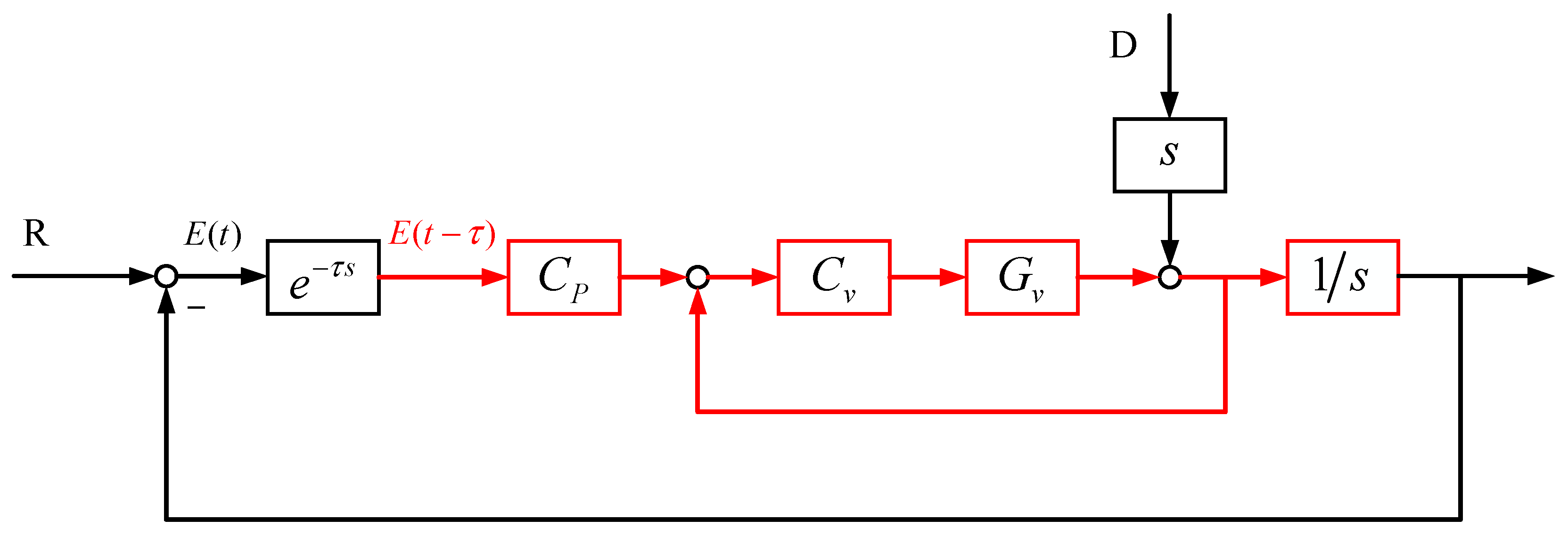
• R: Angular position command of the tracking control system, representing the actual angular position of the target relative to the tracking control system in the geographic coordinate system.
• Y: Angular position response of the tracking control system.
• $C_P$: Position loop controller of the tracking control system.
• $\tau$: Off-target error delay time.
• $C_v$: Velocity loop controller of the tracking control system.
• D: Attitude disturbance of the motion carrier, measured and obtained through inertial navigation.
• $G_v$: Controlled object model for the velocity loop.

Furthermore, the significant temporal gaps in the sampling intervals for off-target deviation between different frame images, caused by the low sampling rate, also contribute to control delays. The lag delay and low sampling rate characteristics of image-based off-target deviations significantly impact the dynamic performance of the control system [5,6]. Therefore, when optimizing electro-optical tracking systems, in addition to enhancements in imaging mechanisms and image processing stages, it is imperative to consider compensation strategies at the control algorithm level to enhance the dynamic performance of the control system.

In recent years, a substantial body of research has been undertaken by numerous scholars in the field of delay compensation. These efforts can be categorized into several aspects. The first category involves treating the control system as a first- or second-order system with a delay component. This approach aims to mitigate the impact of delay on the control system’s dynamic characteristics while ensuring system stability margins. It does so through improvements in PID controller structures (e.g., PID-I controllers [7]) and controller parameter optimization [7,8,9]. Although these methods exhibit some theoretical innovation, they typically require relatively low stability margins (typically around 6 dB), and the research work has remained in the theoretical and simulation stages, with no subsequent reports of engineering application validation for such control methods.

The second category comprises commonly used methods for compensating delay characteristics, involving the application of Smith predictors and their enhanced versions [10,11,12]. For instance, Ren et al. [10] applied the Smith predictor to the velocity loop of an electro-optical tracking system to compensate for the delay in the gyroscope measurement signal. This was achieved by increasing the open-loop control gain to enhance system tracking performance. Bohm et al. [11] introduced a delay compensation algorithm in the disturbance rejection loop of a telescope’s optical components. They estimated disturbance effects within the frequency band of interest based on a model-free approach and employed a method similar to the Smith predictor for disturbance feedforward compensation, thereby enhancing the disturbance rejection capabilities of optical components. Luo et al. [12] combined the Smith predictor with velocity feedforward control to improve control system stability while providing feedforward compensation for delay. Despite the considerable benefits of these typical delay compensation methods based on the Smith predictor, they still exhibit some flaws. For example, the application of the Smith predictor in the velocity loop may conflict with existing disturbance observers or state observers, consequently diminishing the disturbance rejection capabilities of electro-optical tracking systems [13,14]. Model-free delay compensation algorithms are ineffective for handling large delay systems (e.g., delays greater than 15 ms). Some novel control techniques, such as fractional-order control, combined with Smith predictors, have not yet received adequate testing and validation in practical systems [15,16].

Another class of delay compensation methods involves composite control techniques combining velocity feedforward with Kalman filtering. This methodology combines angular feedback signals in either the carrier frame or the geographical frame with the off-target deviation to derive an equivalent angular position command for the target. Kalman filtering is employed to estimate the target’s velocity, and this estimate is then applied to the control system through feedforward methods [17,18,19,20]. These control methods effectively mitigate the impact of delay on the system. However, the selection of the state equations for the Kalman filter remains a subject of discussion, such as the models associated with constant velocity motion [21], Singer models [22], and current statistical models [23].

In summary, the methods discussed can enhance target tracking accuracy to some extent, but they come with their limitations. Smith predictors and related technologies demand a strong prior understanding of the controlled model, and their effectiveness diminishes when the model is time-varying or hard to obtain accurately. Applying velocity feedforward techniques in electro-optical control systems is demanding in terms of the system’s operating environment. In cases where the platform or carrier experiences significant dynamic inertial disturbances and lacks the means to observe carrier angular motion, this technology may not be suitable. Additionally, this approach requires combining with Kalman filtering, which adds computational demands to the control system. This paper introduces a target prediction and tracking control technique that fuses attitude information in multiple spatial reference frames. Leveraging high-frequency inertial navigation attitude data, it captures the angular motion of the electro-optical equipment’s platform. This enables the conversion and fusion of angular position information of the tracked target in various spatial frames, including the imaging frame, carrier frame, and geographic frame. The method effectively addresses the issues of sampling delay and lag inherent in off-target error, and its efficacy is verified from the perspective of control system stability.

In contrast to prior research by scholars, as described earlier, the control technique presented in this paper does not aim to enhance tracking accuracy through controller design, servo hardware design, or the establishment of a priori disturbance models. Instead, it achieves improved tracking accuracy through real-time and precise modeling of the angular motion of the observer’s platform through the introduction of inertial navigation information. This results in enhanced frequency, accuracy, real-time performance, and predictability of the position and velocity setpoint commands in the tracking system.

This represents a significant technological innovation, as it deeply integrates inertial navigation technology with tracking control technology. It is worth noting that this method requires the complete integration of inertial navigation components within the tracking system, not limited to gyroscope components. The proposed approach allows for modeling of target motion in the geographic coordinate system, as depicted in Figure 2. In practical applications, it demonstrates excellent performance when observing high-speed moving targets, such as unmanned boats and drones, at close range.

2. Principles of Target Prediction and Tracking Control Technology Based on Multi-Space Reference Fusion

The target prediction and tracking control technique involving the fusion of attitude information in multiple spatial frames primarily encompasses two main components: Multi-Spatial Frame Attitude Information Fusion and Target Prediction Algorithm.

Step 1: Fusion of attitude information on a multi-space basis

Incorporating additional inertial attitude observations into the tracking control system, the fusion process combines three aspects of information: the off-target signal, platform angular measurements, and inertial signals of the sensitive carrier’s attitude. By projecting these observations, the tracking control system obtains the commanded attitude angle “$r$” in the geodetic reference frame. At the same time, this fusion process reduces the impact of carrier attitude disturbances on the commanded attitude, resulting in an equivalent command signal, $r\left(s\right)$.

$$r\left(s\right)=R{e}^{-\tau s}$$

(1)

In Equation (1), R represents the ideal command signal, $R\left(s\right)$, as depicted in Figure 1. Due to the lag duration, $\tau$, associated with the off-target measurements required for data fusion, the equivalent command signal, $r\left(s\right)$, obtained at this time should reflect the ideal command signal delayed by the lag duration, $\tau$.

Step 2: Target prediction algorithm

The expression obtained from Equation (1) in Step 1 is represented in the time domain as [time-domain expression], adhering to the principle that “the change in off-target quantity in the geodetic reference frame is a small quantity” utilizes the current geodetic frame’s angular response differential as the gradient of the change in the target angular position. In this context, “y” represents the time-domain expression of the angular position response “Y” as shown in Figure 1. This allows the prediction of the target’s angular position command signal at the current moment, and its calculation is given by the following formula:

$$r\left(t\right)=r\left(t-\tau \right)+{\int }_{t-\tau }^t\dot{y}\left(s-\tau \right)ds$$

(2)

This target prediction algorithm leverages the small changes in the off-target deviation to estimate the current–time target angular position command, providing a mechanism for real-time adjustments and improved tracking accuracy.

2.1. Fusion of Attitude Information in a Multi-Space Basis

In the position loop of the tracking control structure illustrated in Figure 1, the off-target deviation undergoes a continuous projection sequence, transitioning from the imaging frame to the carrier frame, then to the geographical frame, and back to the carrier frame. This process involves the transformation of angle error signals across multiple spatial frames, enabling high-frequency interpolation and resampling of the off-target deviation. Given that the multi-spatial frame projection process relies on inertial attitude data, this technology necessitates real-time provision of the tracking control platform base’s attitude information by the Inertial Measurement Unit (IMU).

Figure 3 depicts a schematic diagram of the coordinate transformation during the multi-space basis projection process. The IMU is mounted below the electro-optical tracking axis system, sharing the same azimuth axis as the electro-optical detector. In this setups, the pitch angle is denoted as θ (with the upward direction considered positive), $P_{XY}$ represents the projection of the target’s direction vector $P_Z{\overrightarrow{P}}_{XY}$ on the target surface frame $X_L{O}_L{Y}_L$, and $P_X, P_Y$, and $P_Z$ represent the projection components of the target vector $P_Z{\overrightarrow{P}}_{XY}$ on the three axes, $X_L, Y_L$, and $Z_L$, respectively.

• $b_L$: The target coordinate system, along the direction facing the target, is defined as left, down, and rear.
• $b_p$: The pitch-axis fixed-coordinate system coincides with $b_L$ and is defined as right, forward, and up.
• $b_{p0}$: The pitch-axis zero coordinate system is aligned with $b_p$, differing from the pitch angle $\theta$, and defined in the same manner as the azimuth-zero coordinate system: forward, left, and up.
• $b_v$: The azimuth-axis coordinate system is defined as forward, left, and up.
• $b_{v0}$: The azimuth-zero coordinate system is defined as forward, left, and up.
• $b_s$: The installation base coordinate system is aligned with $b_{v0}$.
• $b_i$: The IMU carrier coordinate system is defined as right, front, and up.
• $n$: The geographical coordinate system is defined as east, north, and up.

2.1.1. Projection Transformation from Target Surface Frame to Geographical Frame

The transformation primarily involves the following coordinate conversions. The transformation relationship between $b_p$ and $b_p{}_0$ can be expressed as follows:

$${\mathit{C}}_{b_p}^{b_{p0}}={\mathit{C}}_X\left({\theta }_{el}\right)$$

(3)

In this context, ${\mathit{C}}_X\left({\theta }_{el}\right)$ and ${\mathit{C}}_{b_v}^{b_{v0}}$ can be related as follows: a rotation around the pitch axis (X-axis) is represented by the symbol ${\theta }_{el}$. The transformation relationship between $b_v$ and $b_{v0}$, the measured angle value for azimuth be represented as ${\theta }_{az}$, can be expressed as follows:

$${\mathit{C}}_{b_v}^{b_{v0}}={\mathit{C}}_Z\left({\theta }_{az}\right)$$

(4)

where ${\mathit{C}}_Z\left({\theta }_{az}\right)$ represents the rotation ${\theta }_{az}$ along the azimuth axis, Z-axis, $b_p$ and $b_L$. The transformation relationship between them is as follows:

$${\mathit{C}}_{b_L}^{b_p}=\left[\begin{array}{ccc}-1& 0& 0\\ 0& 0& -1\\ 0& -1& 0\end{array}\right]$$

(5)

The transformation relationship among $b_{p0}$, $b_v$, $b_{v0}$, and $b_i$ is represented as follows:

$${\mathit{C}}_{b_{p0}}^{b_v}={\mathit{C}}_i^{b_{v0}}=\left[\begin{array}{ccc}0& 1& 0\\ -1& 0& 0\\ 0& 0& 1\end{array}\right]$$

(6)

The projected vector of the target in the target coordinate system is represented as follows: ${\mathit{r}}_P^{b_L}$.

In Figure 3, the corresponding angles of the boresight error are denoted as ${\theta }_X=\angle P_X{P}_Z{O}_L \mathrm{and} {\theta }_Y=\angle P_Y{P}_Z{O}_L$. The relationship is given as follows:

$${\mathit{r}}_P^{b_L}=\overrightarrow{P_{XY}{P}_Z}=\left[\begin{array}{c}-\cos {\theta }_Y\sin {\theta }_X\\ -\sin {\theta }_Y\\ -\cos {\theta }_Y\cos {\theta }_X\end{array}\right]$$

(7)

The projection of the target in the $b_s$-coordinate system is expressed as ${\mathit{r}}_P^{b_s}$.

According to the chain rule of matrix operations:

$${\mathit{r}}_P^{b_s}={\mathit{C}}_{b_{v0}}^{b_s}{\mathit{C}}_{b_v}^{b_{v0}}{\mathit{C}}_{b_{p0}}^{b_v}{\mathit{C}}_{b_p}^{b_{p0}}{\mathit{C}}_{b_L}^{b_p}{\mathit{r}}_P^{b_L}$$

(8)

where ${\mathit{C}}_{b_{v0}}^{b_s}=\mathit{I}$.

The above equation can be derived from (3) to (8) as follows:

$${\mathit{r}}_P^{b_s}=\left[\begin{array}{c}\cos {\theta }_{v0}\cos \theta \cos {\theta }_P\cos {\theta }_X-\sin {\theta }_{v0}\cos {\theta }_P\sin {\theta }_X-\cos {\theta }_{v0}\sin \theta \sin {\theta }_P\\ \sin {\theta }_{v0}\sin \theta \sin {\theta }_P-\cos {\theta }_{v0}\cos {\theta }_P\sin {\theta }_X-\cos \theta \sin {\theta }_{v0}\cos {\theta }_P\cos {\theta }_X\\ \cos \theta \sin {\theta }_P+\sin \theta \cos {\theta }_P\cos {\theta }_X\end{array}\right]$$

(9)

The projection vector ${\mathit{r}}_P^n$ of the target in the geographic coordinate system is given as follows:

$${\mathit{r}}_P^n={\mathit{C}}_i^n{\mathit{C}}_{b_s}^i{\mathit{r}}_P^{b_s}$$

(10)

where ${\mathit{C}}_i^n$ is the attitude matrix of the platform base sensitive to IMU relative to the geographic coordinate system.

2.1.2. Interpolation and Resampling of Off-Target Deviation in the Geographical Frame

The interpolation and resampling of off-target deviation in the geographical frame are based on the spatial coordinate transformation from the target surface frame to the geographical frame. Simultaneously, at the same time step, the pitch angle measurement, azimuth angle measurement, and inertial attitude information of the tracking control system are fused. This fusion process fully utilizes high-sampling-rate angle measurements and inertial attitude data to achieve interpolation and resampling of the low-sampling-rate off-target deviation data. Assuming that the sampling interval of the deflection error is $\mathsf{\Delta }T$, consecutive $T_0$ and $T_1$ moments satisfy the relationship $\mathsf{\Delta }T=T_1-T_0$. In the geographic coordinate system, the change in the target’s deflection error is considered negligible in engineering, i.e., it can be approximated as 0.

$$\frac{{\mathit{r}}_P^n\left(T_1\right)-{\mathit{r}}_P^n\left(T_0\right)}{\mathsf{\Delta }T}\approx 0$$

(11)

Equation (11) indicates that the target’s angular position in the geographic coordinate system remains unchanged between the two consecutive sampling moments (i.e., ${\mathit{r}}_P^n\left(T_0\right)\approx {\mathit{r}}_P^n\left(T_1\right)$), and based on this condition, interpolation and resampling are performed.

At time $T_0$, combining Equations (8) and (10), we obtain the target’s angular vector in the geographic coordinate system at that moment:

$${\mathit{r}}_P^n\left(T_0\right)={\mathit{C}}_i^n\left(T_0\right)\cdot {\mathit{C}}_{b_s}^i\cdot {\mathit{C}}_{b_{v0}}^{b_s}\cdot {\mathit{C}}_{b_v}^{b_{v0}}\left(T_0\right)\cdot {\mathit{C}}_{b_{p0}}^{b_v}\cdot {\mathit{C}}_{b_p}^{b_{p0}}\left(T_0\right)\cdot {\mathit{C}}_{b_L}^{b_p}\cdot {\mathit{r}}_P^{b_L}\left(T_0\right)$$

(12)

Here, the ${\mathit{C}}_{b_p}^{b_{p0}}\left(T_0\right)$, ${\mathit{C}}_{b_v}^{b_{v0}}\left(T_0\right)$, and ${\mathit{C}}_i^n\left(T_0\right)$ are calculated based on the current pitch angle measurement, yaw angle measurement, and inertial attitude data. In this context, we assume that the sampling frequencies of the inertial measurements and angle measurements are both $\mathsf{\Delta }t$, and $\mathsf{\Delta }T=n\mathsf{\Delta }t$ (n is the ratio of the sampling rate of the boresight error (turret off-pointing error) and the inertial navigation system (INS) attitude measurements). Therefore, within two consecutive target deflection sampling moments $\mathsf{\Delta }T$, we have $t_0=T_0, t_1=T_0+\mathsf{\Delta }t$, …, $t_n=T_0+n\mathsf{\Delta }t=T_1$, Equation (12) can be rewritten as follows:

$${\mathit{r}}_P^{b_L}\left(t_0\right)={\mathit{r}}_P^{b_L}\left(T_0\right)={\mathit{C}}_{b_p}^{b_L}\cdot {\mathit{C}}_{b_{p0}}^{b_p}\left(t_0\right)\cdot {\mathit{C}}_{b_v}^{b_{p0}}\cdot {\mathit{C}}_{b_{v0}}^{b_v}\left(t_0\right)\cdot {\mathit{C}}_{b_s}^{b_{v0}}\cdot {\mathit{C}}_i^{b_s}\cdot {\mathit{C}}_n^i\left(t_0\right)\cdot {\mathit{r}}_P^n\left(T_0\right)$$

(13)

Based on Equation ${\mathit{r}}_P^n\left(T_0\right)={\mathit{r}}_P^n\left(T_1\right)$, it can be determined that the resampled off-target signal at time $T_1$ is

$$\begin{gathered} t_0:{\mathit{r}}_P^{b_L}\left(t_0\right)={\mathit{r}}_P^n\left(T_0\right) \\ {t}_1:{\mathit{r}}_P^{b_L}\left(t_1\right)={\mathit{C}}_{b_p}^{b_L}\cdot {\mathit{C}}_{b_{p0}}^{b_p}\left(t_1\right)\cdot {\mathit{C}}_{b_v}^{b_{p0}}\cdot {\mathit{C}}_{b_{v0}}^{b_v}\left(t_1\right)\cdot {\mathit{C}}_{b_s}^{b_{v0}}\cdot {\mathit{C}}_i^{b_s}\cdot {\mathit{C}}_n^i\left(t_1\right)\cdot {\mathit{r}}_P^n\left(T_0\right) \\ {t}_2:{\mathit{r}}_P^{b_L}\left(t_2\right)={\mathit{C}}_{b_p}^{b_L}\cdot {\mathit{C}}_{b_{p0}}^{b_p}\left(t_2\right)\cdot {\mathit{C}}_{b_v}^{b_{p0}}\cdot {\mathit{C}}_{b_{v0}}^{b_v}\left(t_2\right)\cdot {\mathit{C}}_{b_s}^{b_{v0}}\cdot {\mathit{C}}_i^{b_s}\cdot {\mathit{C}}_n^i\left(t_2\right)\cdot {\mathit{r}}_P^n\left(T_0\right) \\ \dots \dots \\ {t}_n=T_1:{\mathit{r}}_P^{b_L}\left(t_n\right)={\mathit{C}}_{b_p}^{b_L}\cdot {\mathit{C}}_{b_{p0}}^{b_p}\left(t_n\right)\cdot {\mathit{C}}_{b_v}^{b_{p0}}\cdot {\mathit{C}}_{b_{v0}}^{b_v}\left(t_n\right)\cdot {\mathit{C}}_{b_s}^{b_{v0}}\cdot {\mathit{C}}_i^{b_s}\cdot {\mathit{C}}_n^i\left(t_n\right)\cdot {\mathit{r}}_P^n\left(T_1\right) \end{gathered}$$

(14)

These equations summarize the comparison of the target angular vectors before and after inertial interpolation and resampling, as shown in the following table.

Table 1. Comparison of target angular position vectors before and after interpolation and resampling.

Off-Target Deviation Sampling Time (Low-Frequency)	IMU Sampling Time (High-Frequency)	Off-Target Deviation before Resampling	Equivalent Target Angular Position Vector after Resampling
$T_0$	$t_{00}$	${\mathit{r}}_P^{b_L}\left(T_0\right)$	${\mathit{C}}_{b_p}^{b_L}{\mathit{C}}_{b_{p0}}^{b_p}\left(t_{00}\right){\mathit{C}}_{b_v}^{b_{p0}}{\mathit{C}}_{b_{v0}}^{b_v}\left(t_{00}\right){\mathit{C}}_{b_s}^{b_{v0}}{\mathit{C}}_i^{b_s}{\mathit{C}}_n^i\left(t_{00}\right){\mathit{r}}_P^n\left(T_0\right)$
	$t_{01}$		${\mathit{C}}_{b_p}^{b_L}{\mathit{C}}_{b_{p0}}^{b_p}\left(t_{01}\right){\mathit{C}}_{b_v}^{b_{p0}}{\mathit{C}}_{b_{v0}}^{b_v}\left(t_{01}\right){\mathit{C}}_{b_s}^{b_{v0}}{\mathit{C}}_i^{b_s}{\mathit{C}}_n^i\left(t_{01}\right){\mathit{r}}_P^n\left(T_0\right)$
	…		…
	$t_{0n}$		${\mathit{C}}_{b_p}^{b_L}{\mathit{C}}_{b_{p0}}^{b_p}\left(t_{0n}\right){\mathit{C}}_{b_v}^{b_{p0}}{\mathit{C}}_{b_{v0}}^{b_v}\left(t_{0n}\right){\mathit{C}}_{b_s}^{b_{v0}}{\mathit{C}}_i^{b_s}{\mathit{C}}_n^i\left(t_{0n}\right){\mathit{r}}_P^n\left(T_0\right)$
$T_1$	$t_{10}$	${\mathit{r}}_P^{b_L}\left(T_1\right)$	${\mathit{C}}_{b_p}^{b_L}{\mathit{C}}_{b_{p0}}^{b_p}\left(t_{10}\right){\mathit{C}}_{b_v}^{b_{p0}}{\mathit{C}}_{b_{v0}}^{b_v}\left(t_{10}\right){\mathit{C}}_{b_s}^{b_{v0}}{\mathit{C}}_i^{b_s}{\mathit{C}}_n^i\left(t_{10}\right){\mathit{r}}_P^n\left(T_1\right)$
	$t_{11}$		${\mathit{C}}_{b_p}^{b_L}{\mathit{C}}_{b_{p0}}^{b_p}\left(t_{11}\right){\mathit{C}}_{b_v}^{b_{p0}}{\mathit{C}}_{b_{v0}}^{b_v}\left(t_{11}\right){\mathit{C}}_{b_s}^{b_{v0}}{\mathit{C}}_i^{b_s}{\mathit{C}}_n^i\left(t_{11}\right){\mathit{r}}_P^n\left(T_1\right)$
	…		…
	$t_{1n}$		${\mathit{C}}_{b_p}^{b_L}{\mathit{C}}_{b_{p0}}^{b_p}\left(t_{1n}\right){\mathit{C}}_{b_v}^{b_{p0}}{\mathit{C}}_{b_{v0}}^{b_v}\left(t_{1n}\right){\mathit{C}}_{b_s}^{b_{v0}}{\mathit{C}}_i^{b_s}{\mathit{C}}_n^i\left(t_{1n}\right){\mathit{r}}_P^n\left(T_1\right)$
…	…	…	…
$T_m$	$t_{m0}$	${\mathit{r}}_P^{b_L}\left(T_m\right)$	${\mathit{C}}_{b_p}^{b_L}{\mathit{C}}_{b_{p0}}^{b_p}\left(t_{m0}\right){\mathit{C}}_{b_v}^{b_{p0}}{\mathit{C}}_{b_{v0}}^{b_v}\left(t_{m0}\right){\mathit{C}}_{b_s}^{b_{v0}}{\mathit{C}}_i^{b_s}{\mathit{C}}_n^i\left(t_{m0}\right){\mathit{r}}_P^n\left(T_m\right)$
	$t_{m1}$		${\mathit{C}}_{b_p}^{b_L}{\mathit{C}}_{b_{p0}}^{b_p}\left(t_{m1}\right){\mathit{C}}_{b_v}^{b_{p0}}{\mathit{C}}_{b_{v0}}^{b_v}\left(t_{m1}\right){\mathit{C}}_{b_s}^{b_{v0}}{\mathit{C}}_i^{b_s}{\mathit{C}}_n^i\left(t_{m1}\right){\mathit{r}}_P^n\left(T_m\right)$
	…		…
	$t_{mn}$		${\mathit{C}}_{b_p}^{b_L}{\mathit{C}}_{b_{p0}}^{b_p}\left(t_{mn}\right){\mathit{C}}_{b_v}^{b_{p0}}{\mathit{C}}_{b_{v0}}^{b_v}\left(t_{mn}\right){\mathit{C}}_{b_s}^{b_{v0}}{\mathit{C}}_i^{b_s}{\mathit{C}}_n^i\left(t_{mn}\right){\mathit{r}}_P^n\left(T_m\right)$

illustrates the fundamental principle of interpolation and resampling, which involves increasing the update frequency of the target angular position vector by utilizing high-frequency angle measurements and inertial attitude information. Taking a typical maritime platform’s electro-optical tracking system as an example, the update frequencies for angular displacements in the axis system and inertial attitude are typically 1000 Hz, while the update frequency for off-target deviation is less than 100 Hz. The resampling process illustrated in Table 1 enables an increase in the update frequency of the off-target deviation to 1000 Hz.

2.1.3. Generation of High-Sampling-Rate Elevation and Azimuth Angles

During the process of back-projection from the geographical frame to the carrier frame, it is necessary to consider the updates of inertial and angle measurement signals within the off-target deviation lag delay time. Assuming the off-target deviation lag time is denoted as τ, when projecting from the target surface frame to the geographical frame, inertial and angle measurement data from a time earlier than τ are used. In contrast, during the back-projection from the geographical frame to the carrier frame, the inertial and angle measurement data from the current time are used to address the lag delay of the off-target deviation, in addition to the sampling delay.

As given in

Table 2. Time sequence comparison of forward and backward projection.

Current Time	Time Corresponding to the Off-Target Deviation	Off-Target Deviation Values	Target Angular Vector Projected into the Geographical Frame during forward Projection	Target Angular Vector after Back-Projection into the Carrier Frame
$t_0$	$T_0-\tau$	${\mathit{r}}_P^{b_L}\left(T_0-\tau \right)$	${\mathit{r}}_P^n\left(t_0-\tau \right)$	${\mathit{C}}_i^{b_s}{\mathit{C}}_n^i\left(t_0\right){\mathit{r}}_P^n\left(t_0-\tau \right)={\mathit{r}}_P^{b_s}\left(t_0\right)$
$t_1$			${\mathit{r}}_P^n\left(t_1-\tau \right)$	${\mathit{C}}_i^{b_s}{\mathit{C}}_n^i\left(t_1\right){\mathit{r}}_P^n\left(t_1-\tau \right)={\mathit{r}}_P^{b_s}\left(t_1\right)$
$t_2$			${\mathit{r}}_P^n\left(t_2-\tau \right)$	${\mathit{C}}_i^{b_s}{\mathit{C}}_n^i\left(t_2\right){\mathit{r}}_P^n\left(t_2-\tau \right)={\mathit{r}}_P^{b_s}\left(t_2\right)$
…			…	…
$t_n$			${\mathit{r}}_P^n\left(t_n-\tau \right)$	${\mathit{C}}_i^{b_s}{\mathit{C}}_n^i\left(t_n\right){\mathit{r}}_P^n\left(t_n-\tau \right)={\mathit{r}}_P^{b_s}\left(t_n\right)$

, at time $t_i$ ($i=0~n$), when projecting back to the carrier system, the selected geodetic system’s target angle vector is the same as the one at time $t_i-\tau$. Therefore, the prerequisite for generating high-sampling-rate elevation and azimuth is that, within the lag time $\tau$, the change in the target’s angular position in the geodetic system can be neglected. It must satisfy the condition that ${\mathit{r}}_P^n\left(t_i-\tau \right)={\mathit{r}}_P^n\left(t_i\right)$($i=0~n$), as shown in Equation (11).

Furthermore, the target angle vector in the carrier system can be expressed in terms of elevation angle $H_s$ and azimuth angle $A_s$:

$${\mathit{r}}_P^{b_s}\left(t\right)=\left[\begin{array}{c}\cos H_s\cos A_s\\ -\cos H_s\sin A_s\\ \sin H_s\end{array}\right]$$

(15)

Hence, through the fusion of high-sampling-rate data from angle measurement and inertial navigation, high-sampling-rate elevation angle $H_s$ and azimuth angle $A_s$ can be obtained, thereby providing the tracking and control system with effective, real-time command reference signals without delay.

$$\{\begin{array}{l}{H}_s=\arcsin r_{P,z}^{b_s}\left(t\right)\\ A_s=\arctan 2\left(-r_{P,y}^{b_s}\left(t\right),r_{P,x}^{b_s}\left(t\right)\right)\end{array}$$

(16)

2.2. Target Prediction Algorithm

Because, within the lag delay time τ, the change in the target’s angular position in the geographical frame is not sufficiently small, especially for high-mobility and close-range targets—such as a target at a distance of 180 m and a speed of 20 knots—when the off-target deviation lags by 100 ms, the change in the target’s angular displacement can reach 0.3° (≈5 mrad). This 0.3° cannot be compensated for using the multi-spatial frame attitude fusion technique mentioned earlier. Therefore, the target tracking algorithm must address the situation of lag delay.

To overcome this challenge, a prediction algorithm for the target’s angular position in the geographical frame is proposed. At the current time t, the target’s angular position in the geographical frame is denoted as $r\left(t\right)$, and the relationship is expressed as follows:

$$r\left(t\right)=r\left(t-\tau \right)+{\int }_{t-\tau }^t\dot{r}\left(s\right)ds$$

(17)

In Equation (17), ${\int }_{t-\tau }^t\dot{r}\left(s\right)ds$ represents the change in angular position within the time interval $\left[\begin{array}{cc}t-\tau & t\end{array}\right]$, where $\dot{r}\left(s\right)$ is the gradient of the angular position change. Considering the relationship between the off-target deviation and angular response, and since the off-target deviation $e\left(t\right)$ in the geographical frame $e\left(t\right)=r\left(t\right)-y\left(t\right)$ can be neglected, Equation (17) can be transformed into:

$$\widehat{r}\left(t\right)=r\left(t-\tau \right)+{\int }_{t-\tau }^t\dot{y}\left(s\right)ds$$

(18)

Neglecting changes within the delay time τ, we can set $\dot{y}(t-\tau )\approx \dot{y}(t)$. In this case, Equation (18) can be written as follows:

$$\widehat{r}\left(t\right)=r\left(t-\tau \right)+{\int }_{t-2\tau }^{t-\tau }\dot{y}\left(s\right)ds=r\left(t-\tau \right)+{\int }_{t-\tau }^t\dot{y}\left(s-\tau \right)ds$$

(19)

With Equation (19), the prediction can provide an estimate of the target’s angle reference signal without delay at the current time, denoted as $\widehat{R}(t)\approx r(t)$. In a discrete system, this can be represented as follows:

$${\widehat{R}}_0\left(k\right)=R_{-\tau }\left(k\right)+\frac{y\left(k\right)-y\left(k-n\right)}{n{T}_s}\tau$$

(20)

3. Control System Design and Analysis of Target Prediction Algorithm Based on Multi-Spatial Frame Attitude Information Fusion

3.1. Control System Design for Target Prediction Algorithm Based on Multi-Spatial Frame Fusion

The integration of the multi-spatial frame attitude information fusion algorithm and the target prediction algorithm is reflected in the block diagram of the tracking control system, as shown in Figure 4.

In Figure 4, the meanings of the symbols R, Y, $C_P$, $\tau$, D, $C_v$, and $G_v$ are the same as in Figure 1. Additional symbol explanations are as follows:

• E: Control error in angular position.
• ${\widehat{R}}_{-\tau }$: Estimated target angular position relative to the geodetic reference frame at a lag, τ.
• $\widehat{R}$: Estimated target angular position relative to the geodetic reference frame at the current time t.
• ${\tau }_m$: Pre-measured time delay associated with the off-target measurements. The discussion in this paper is based on the condition of having lag, ${\tau }_m\approx \tau$.

The implementation workflow of the target prediction algorithm based on multi-spatial frame attitude fusion is as follows:

(1) Through the multi-spatial frame projection transformation from the target surface frame to the carrier frame and then to the geographical frame, estimate the command signal, ${\widehat{R}}_{-\tau }$ at the lagged time τ, thereby overcoming the sampling delay of the off-target deviation.

By performing a brief derivation according to Figure 4, we can set the position loop controller gain as $C_p=1$. Considering that the bandwidth of the velocity loop control is significantly higher than that of the position loop, and within its bandwidth, the closed-loop velocity model is approximately 1. Therefore, we have:

$$e\left(t-\tau \right)=r\left(t-\tau \right)-y\left(t-\tau \right)$$

(21)

$$u\left(t\right)+\dot{d}\left(t\right)=\dot{y}\left(t\right)$$

(22)

The estimated value of $\widehat{r}\left(t-{\tau }_m\right)$, which is the ${\widehat{R}}_{-\tau }$ (as shown in Figure 4), is as follows:

$$\begin{array}{c}\widehat{r}(t-{\tau }_m)=e(t-\tau )+\widehat{y}(t-{\tau }_m)\\ \hspace{1em}\hspace{1em}\hspace{1em} =r(t-\tau )-y(t-\tau )+\widehat{y}(t-{\tau }_m)\end{array}$$

(23)

Since the angle response values $\widehat{y}\left(t-{\tau }_m\right)$ obtained in this paper encompass both angle measurements ${\int }_0^{t}u\left(s-{\tau }_m\right)ds$ in the carrier frame and the attitude of the carrier platform $d\left(t-{\tau }_m\right)$ measured by inertial sensors, when the prediction is made with a known delay time τ (i.e., ${\tau }_m\approx \tau$ is known), in combination with Equation (22), we have $\widehat{y}\left(t-{\tau }_m\right)=y\left(t-\tau \right)$. Consequently, the estimated value $\widehat{r}\left(t-{\tau }_m\right)$ in Equation (23) can accurately reconstruct the true command signal at the lagged time $r\left(t-\tau \right)$, meaning $\widehat{r}\left(t-{\tau }_m\right)=r\left(t-\tau \right)$. By utilizing the target prediction algorithm to estimate the current–time command signal $\widehat{R}\approx r$, the system overcomes the lag delay in the original off-target deviation signal. At this point, Equation (19) is rewritten as follows:

$$\begin{array}{cc}\hfill \widehat{r}(t)& =\widehat{r}(t-\tau )+{\displaystyle {\int }_{t-\tau }^t\dot{\widehat{y}}(s-\tau )ds}\hfill \\ & =r(t-\tau )+{\displaystyle {\int }_{t-\tau }^t\dot{y}(s-\tau )ds}\end{array}$$

(24)

The above equation can be derived from (3) to (8) as follows:

By using the attitude signal D provided by the inertial measurement unit (IMU) and applying a back-projection transformation, the elevation and azimuth angles relative to the carrier frame at the current time can be obtained. This, in turn, allows for the determination of the angular position error relative to the carrier frame. This angular position error is equivalent to the target off-target deviation $\widehat{E}$ after interpolation and delay compensation. After high-gain control in the velocity loop to suppress system disturbances, the final output is the target angular response value in the geographical frame, denoted as Y.

The entire control process described above utilizes the “attitude transformation in multiple spatial frames” to unify physical quantities to the current time as a “common time reference”, as shown in

Table 3. Description of various physical quantities in the entire control process.

Physical Quantities	Spatial Reference Frame	Time Reference Frame	Remark
R: Angle position of the target	Geographic frame	The present moment	Cannot be directly obtained.
E: Angle position error of the target	Geographic frame	The present moment	Cannot be directly obtained.
$E{e}^{-\tau s}:$ Off-target deviation	Target frame	The delayed time	The actual inputs to the system are subject to sampling and lag delay.
${\widehat{R}}_{-\tau }:$ Estimated target angular position	Geographic frame	The delayed time	After the forward projection transformation from the target surface frame to the carrier frame and then to the geographic frame, the lagged angular measurements and inertial navigation data are used.
$\widehat{R}:$ Estimated target angle position	Geographic frame	The present moment	After applying the target prediction algorithm
$\widehat{E}:$ Estimated target angular position error	Carrier frame	The present moment	Following the transformation from the geographic frame to the carrier frame, utilizing the current moment’s inertial navigation information, the subsequent control inputs for tracking are determined.

.

3.2. Algorithm Stability and Error Analysis

3.2.1. Control System Stability Analysis

Due to the significantly smaller magnitude of the control error E in the geodetic reference frame compared to the target’s angular position R, Equation (24) can be transformed into its Laplace domain (S-domain) representation as follows:

$$\begin{array}{cc}\hfill \widehat{R}(s)& =\widehat{R}(s)e^{-\tau s}+\widehat{Y}(s)e^{-\tau s}{\tau }_{m}s\hfill \\ & =\widehat{R}(s)e^{-\tau s}(1+{\tau }_{m}s)\hfill \\ & \approx \widehat{R}(s)e^{-\tau s}{e}^{{\tau }_{m}s}\hfill \end{array}$$

(25)

Thus, the transfer function within the dashed box in Figure 4 is given by:

$$G\left(s\right)=\frac{\frac{C_p}{\left(1+\frac{C_p}{s}\right)s}{e}^{{\tau }_{m}s}}{1-\frac{C_p}{\left(1+\frac{C_p}{s}\right)s}{e}^{{\tau }_{m}s}{e}^{-{\tau }_{m}s}}=\frac{C_p}{s}{e}^{{\tau }_{m}s}$$

(26)

Furthermore, we can derive the closed-loop transfer function of the control system as shown in Figure 4 to be:

$$H\left(s\right)=\frac{G\left(s\right)e^{-\tau s}}{1+G\left(s\right)e^{-\tau s}}=\frac{\frac{C_p}{s}{e}^{{\tau }_{m}s}{e}^{-\tau s}}{1+\frac{C_p}{s}{e}^{{\tau }_{m}s}{e}^{-\tau s}}\approx \frac{C_p}{s+C_p}$$

(27)

Analyzing Equation (27), it can be observed that by designing the controller, i.e., $\left|C_p\right|>0$, ensuring that the characteristic polynomial in Equation (27) is Hurwitz, the control system is stable. Consequently, the stability of the system depicted in Figure 4 is not affected by the time delay characteristics.

3.2.2. Algorithm Error Analysis and Comparison

A comparison is made between this technique and the improved Smith predictor method based on off-target deviation and model output fusion [10]. The angle reference values estimated by the improved Smith predictor are as follows:

$${\widehat{r}}_0\left(t\right)=r\left(t-\tau \right)-d\left(t-\tau \right)$$

(28)

In this case, the estimation error of the improved Smith predictor method is given by:

$${\widehat{e}}_0\left(t\right)=r\left(t\right)-{\widehat{r}}_0\left(t\right)=d\left(t-\tau \right)+{\int }_{t-\tau }^t\dot{y}\left(s\right)ds$$

(29)

Analyzing Equation (29), it is evident that the estimation error comprises two sources of error: the carrier platform motion attitude $d\left(t-\tau \right)$ that cannot be measured by the original tracking control system and the angular difference within the delay time $\left[\begin{array}{cc}t-\tau ,& t\end{array}\right]$. In the case of a moving base motion platform and highly maneuverable detection targets, these two sources of error will be significant.

Similarly, the prediction error obtained in this paper is given by:

$$\widehat{e}\left(t\right)={\int }_{t-\tau }^t\left[\dot{y}\left(s\right)-\dot{y}\left(s-\tau \right)\right]ds$$

(30)

Similarly, the prediction error obtained in this paper is given by:

Analyzing Equation (30), it is evident that the prediction error only contains the difference between the angle gradients of the two adjacent sampling delay periods, which are represented as $\left[\begin{array}{cc}t-2\tau & t-\tau \end{array}\right]$ and $\left[\begin{array}{cc}t-\tau & t\end{array}\right]$. When the target is in uniform motion or exhibits low acceleration (including uniform acceleration or low-frequency periodic motion, etc.), $\dot{y}\left(t\right)-\dot{y}\left(t-\tau \right)=o\left(t\right)$. In such cases, the accuracy of this paper’s prediction algorithm will be significantly higher than the original improved Smith predictor technique.

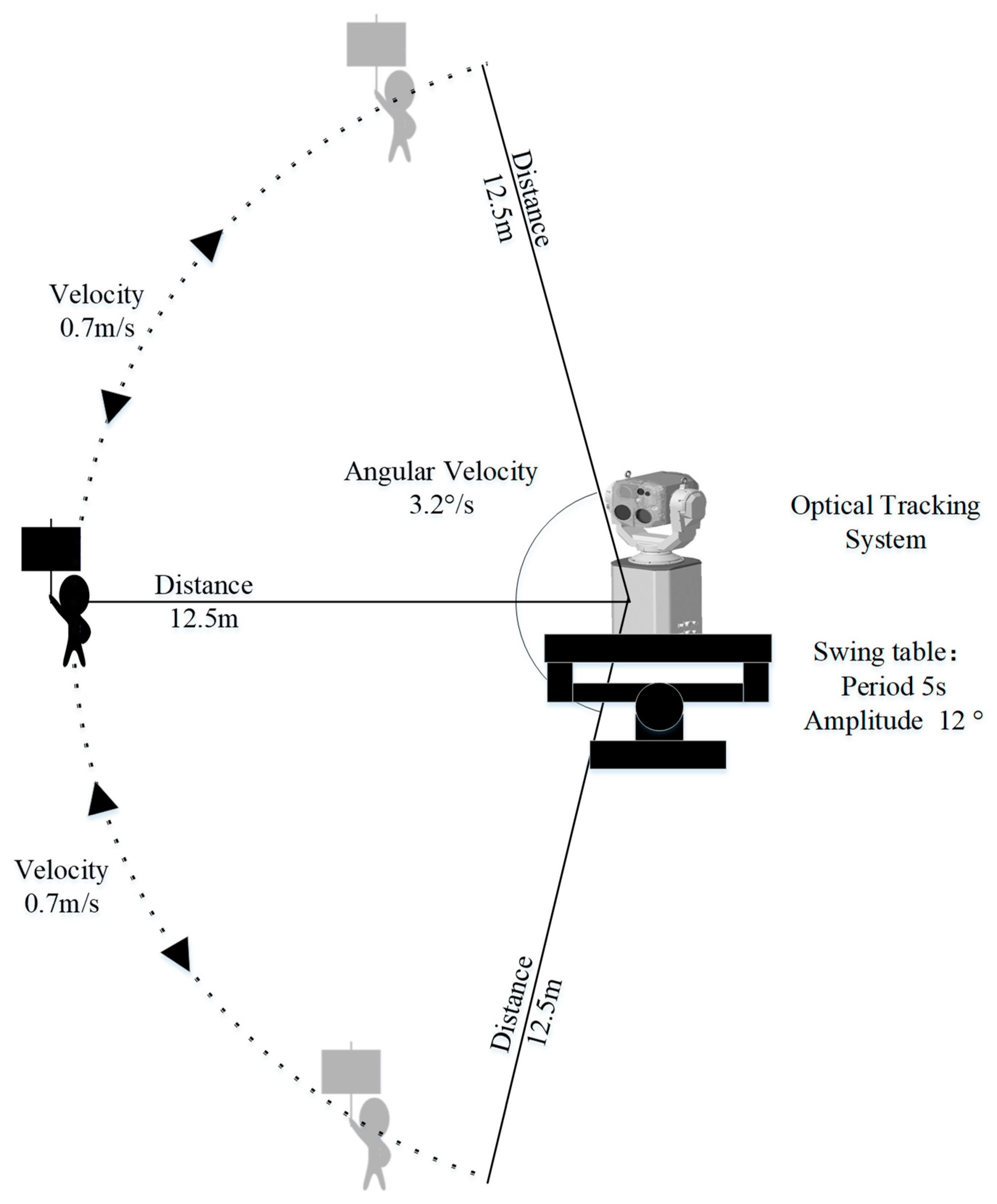
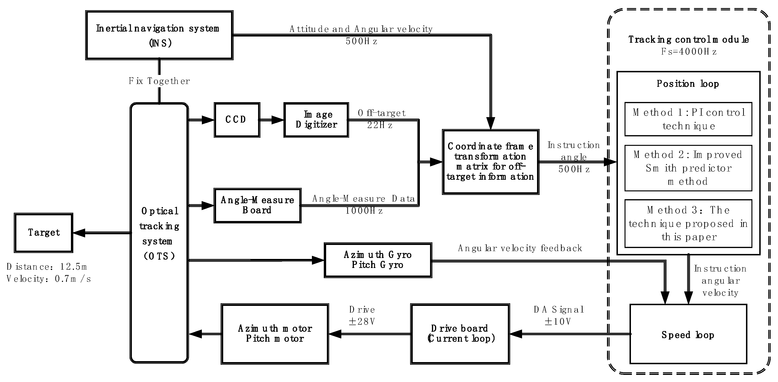
4. Experimental Testing

4.1. Test Conditions

Conducting predictive tracking tests on a dual-loop optical-electronic tracking system installed on a marine-based gyroscope platform, the equipment is mounted on a swivel platform, and the physical representation of the equipment is illustrated in Figure 5.

The swivel platform generates simultaneous pitch and azimuth oscillations with a period of 5 s and an amplitude of 12 degrees. The tracking system is used to track a horizontally moving target, which is handheld by a test operator. The moving target is positioned at a distance of 12.5 m from the optical sensor head and moves back and forth at a speed of 0.7 m/s in a direction perpendicular to the optical axis. The testing scenario is depicted in Figure 6.

The predictive tracking test was conducted using a dual-loop optical tracking system, with a specific type of marine theodolite as the target object. A swing table was employed to induce simultaneous pitch and yaw motions with a 5 s period and a 12-degree amplitude. It is worth noting that these dynamic conditions simulate the equipment’s tracking performance when monitoring a moving target at a distance of 180 m with a speed of 20 knots. The test setup is depicted in Figure 7. The servo frequency of the controller is 4000 Hz, and the update rate of carrier attitude information provided by the inertial system is 500 Hz, while the sampling rate of angle measurements and gyroscope information is 1000 Hz.

4.2. Test Results

The measured tracking characteristics obtained with three different tracking control methods, including the PI control technique, the improved Smith predictor technique (i.e., tracking control technique based on inertial information assistance), and the target prediction control technique based on multi-space attitude fusion proposed in this paper, were obtained and compared. High-gain control was used in the velocity loop for all three tracking control methods.

Table 4. List of controller parameter values.

Position Loop
	Control Parameters	PI Control Technique	Improved Smith Predictor Method	The Control Technique Proposed in This Paper
Pitch axis	$K_p$	0.15	0.15	0.15
	$K_I$	11.5	46	137.5
Azimuth axis	$K_p$	0.15	0.15	0.15
	$K_I$	11.5	46	137.5
Velocity Loop
Pitch axis	$K_p$	8	8	8
	$K_I$	100	100	100
Azimuth axis	$K_p$	30	30	30
	$K_I$	400	400	400

makes it evident that the target prediction control technique based on multi-space attitude fusion can achieve higher control gains compared to the improved Smith predictor technique. This is because the target prediction control technique based on multi-space attitude fusion further eliminates the effects of delay and latency compared to the improved Smith predictor technique.

The test results are compared in Figure 8.

Analyzing the test data presented in Figure 8, it becomes apparent that the target prediction control technique, as proposed in this paper and based on multi-space attitude fusion, surpasses the performance of the other two control techniques. In contrast, both the PI control and the improved Smith predictor technique exhibit noticeable tracking delays. This is primarily due to the target’s motion during the update period of the off-target quantity, leading to angular displacement errors that conventional feedback controllers struggle to compensate for. Furthermore, the swifter the target’s motion, the more pronounced the lag in the off-target quantity. Furthermore, the reason the improved Smith predictor technique does not perform as well as the PI control technique is that, despite using current inertial data for the azimuth angle after high-frequency interpolation, it still has to use the off-target quantity data from the previous update time of the off-target quantity. This introduces additional angular position errors during the space-based transformation, and this error is also something that the feedback controller cannot compensate for. Furthermore, the target tracking accuracy using the three control techniques has been statistically analyzed, as shown in

Table 5. Comparison of target tracking accuracy among three control techniques.

Control Technique	Tracking Accuracy (RMS)
PI control technique	1.8 mrad
Improved Smith predictor	5.8 mrad
Target prediction and tracking control technique based on multi-space frame attitude fusion	633 μrad

.

Experimental data description: The data presented above were obtained under the same conditions, with the target located approximately 12.5 m away from the optical-electronic system. Over a 6 s duration, the target moved at a speed of 0.7 m/s in a direction perpendicular to the optical axis.

Analyzing the test data presented in Figure 8 and Table 5 leads to the following conclusions:

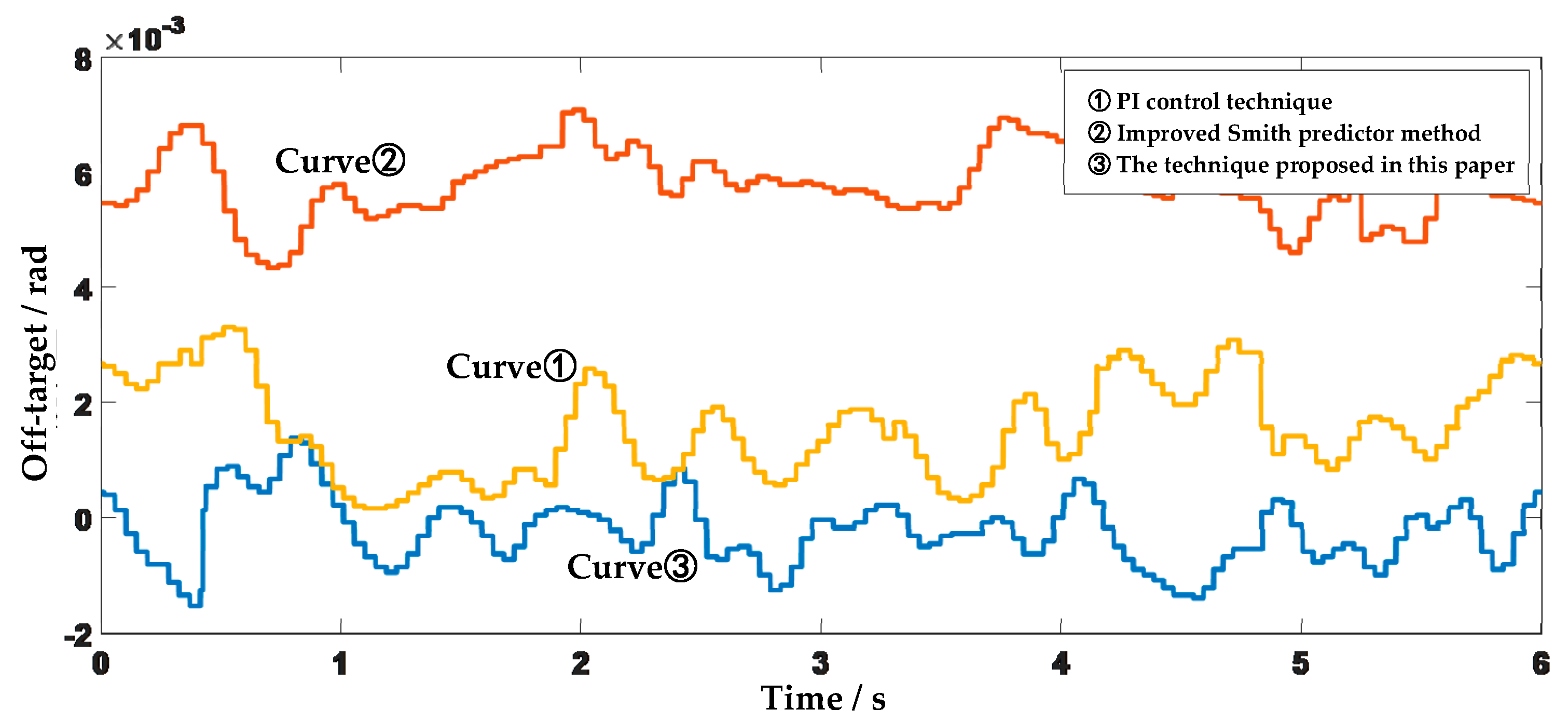
• The target prediction and tracking control technique proposed in this paper, based on multi-space-based attitude fusion, is significantly superior to the other two control techniques. With PI control and the improved Smith predictor technique, when the target is moving at a constant speed, there is a consistent deviation in the target tracking error curve, indicating a noticeable tracking lag.
• In the case of PI control, during the off-target measurement update time, both the angular motion of the optical-electronic device itself and the linear motion of the target can result in angular displacement errors that conventional feedback controllers are unable to compensate for.
• For the improved Smith predictor technique, using gyro information for external disturbance estimation can suppress the interference caused by the angular motion of the optical-electronic device itself. However, since there is no prediction of the target’s linear motion trajectory, when tracking high-speed moving targets, it can actually reinforce the tracking of the lagged target position, resulting in more noticeable tracking lag errors.
• The technique proposed in this paper has advantages over PI control and the improved Smith predictor technique. It leverages real-time measurements from inertial navigation information to compensate for the impact of the angular motion of the optical-electronic device on tracking accuracy. Additionally, it establishes a target motion trajectory model in the relatively stable geodetic coordinate system to compensate for the impact of target movement on tracking accuracy.

5. Conclusions

In conclusion, the challenge of achieving accurate tracking in optical-electronic tracking devices, particularly when dealing with highly maneuverable targets, is accentuated by the presence of off-target measurement delays. In response to this issue, this paper has introduced a target prediction and tracking control technique rooted in multi-space state fusion. This novel technique augments the existing optical-electronic tracking control system by incorporating high-frequency inertial navigation attitude information, alongside angular feedback signals and off-target measurements. It efficiently transforms and amalgamates the measured target angular displacement signals across various spatial frames, encompassing the imaging frame, the platform frame, and the geodetic frame. By doing so, it bridges the gap between discrete and high-discrepancy off-target measurement signals, effectively reducing the sampling delay in off-target measurements. Furthermore, through its ability to predict the target’s angular position, this technique contributes to a further reduction in off-target measurement lag. The results of testing conducted on a specific optical-electronic tracking platform when tracking highly maneuverable targets clearly illustrate the superiority of the control technique proposed in this paper. It enhances target tracking accuracy by a remarkable threefold compared to existing techniques. Under identical experimental conditions, the statistical values of off-target measurements are reduced from 1.8 mrad to 633 μrad.

References

1. Hou, M.L.; Liu, Y.R.; Xing, S.B.; Su, L.Y. Study of intelligent diagnosis system for photoelectric tracking devices based on multiple knowledge representation. Adv. Mater. Res. 2011, 179, 602–607. [Google Scholar] [CrossRef]
2. Li, T.H.; Xiang, D.Q. Research and Design of Photoelectric Solar Tracking System. Adv. Eng. Forum 2012, 4, 115–120. [Google Scholar] [CrossRef]
3. Masten, M.K. Inertially stabilized platforms for optical imaging systems. IEEE Control Syst. Mag. 2008, 28, 47–64. [Google Scholar]
4. Hilkert, J.M. Inertially stabilized platform technology concepts and principles. IEEE Control Syst. Mag. 2008, 28, 26–46. [Google Scholar]
5. Tang, T.; Mao, J.; Chen, H.; Fu, C.; Yang, H.; Ren, G.; Yang, W.; Qi, B.; Cao, L.; Zhang, M.; et al. A review on precision control methodologies for optical-electric tracking control system. Opto-Electron. Eng. 2020, 47, 200315. [Google Scholar]
6. Ekstrand, B. Tracking filters and models for seeker applications. IEEE Trans. Aerosp. Electron. Syst. 2001, 37, 965–977. [Google Scholar] [CrossRef]
7. Tao, T.; Ma, J.; Ren, G. PID-I controller for of charge coupled device-based tracking loop for fast-steering mirror. Opt. Eng. 2011, 50, 043002. [Google Scholar]
8. Srivastava, S.; Pandit, V.S. A PI/PID controller for time delay systems with desired closed loop time response and guaranteed gain and phase margins. J. Process Control 2016, 37, 70–77. [Google Scholar] [CrossRef]
9. Amini, E.; Rahmani, M. Stabilizing PID controller for time-delay systems with guaranteed gain and phase margins. Int. J. Syst. Sci. 2022, 53, 1004–1016. [Google Scholar] [CrossRef]
10. Ren, W.; Luo, Y.; He, Q.N. Stabilization Control of Electro-optical Tracking System with Fiber-Optic Gyroscope Based on Modified Smith Predictor Control Scheme. IEEE Sens. J. 2018, 99, 1. [Google Scholar]
11. Böhm, M.; Pott, J.U.; Kürster, M.; Sawodny, O.; Defrere, D.; Hinz, P. Delay compensation for Real time Disturbance estimation at extremely large telescope. IEEE Trans. Control Syst. Technol. 2016, 25, 1384–1394. [Google Scholar] [CrossRef]
12. Luo, Y.; Xue, W.; He, W.; Nie, K.; Mao, Y.; Guerrero, J.M. Delay-Compound-Compensation Control for Photoelectric Tracking System Based on Improved Smith Predictor Scheme. IEEE Photonics J. 2022, 14, 6625708. [Google Scholar] [CrossRef]
13. Sariyildiz, E.; Ohnishi, K. A guide to design disturbance observer. J. Dyn. Syst. Meas. Control 2014, 136, 11–21. [Google Scholar] [CrossRef]
14. Wang, L.; Su, J. Robust disturbance rejection control for attitude tracking of an air-craft. IEEE Trans. Control Syst. Technol. 2015, 23, 2361–2368. [Google Scholar] [CrossRef]
15. İçmez, Y.; Can, M.S. Smith Predictor Controller Design Using the Direct Synthesis Method for Unstable Second-Order and Time-Delay Systems. Processes 2023, 11, 941. [Google Scholar] [CrossRef]
16. Ghorbani, M.; Tavakoli-Kakhki, M.; Tepljakov, A. Robust stability analysis of smith predictor-based interval fractional-order control systems: A case study in level control process. IEEE/CAA J. Autom. Sin. 2022, 10, 762–780. [Google Scholar] [CrossRef]
17. Tang, T.; Cai, H.; Huang, Y.; Ren, G. Combined line-of-sight error and angular position to generate feedforward control for a charge-coupled device–based tracking loop. Opt. Eng. 2015, 54, 105107. [Google Scholar] [CrossRef]
18. Tang, T.; Tian, T.; Zhong, D.J.; Fu, C.Y. Combining Charge Couple Devices and Rate Sensors for the Feedforward Control System of a Charge Coupled Device Tracking Loop. Sensors 2016, 16, 968. [Google Scholar] [CrossRef]
19. Xie, R.; Zhang, T.; Li, J.; Dai, M. Compensating Unknown Time-Varying Delay in Opto-Electronic Platform Tracking Servo System. Sensors 2017, 17, 1071. [Google Scholar] [CrossRef]
20. Luo, Y.; Ren, W.; Huang, Y.; He, Q.J.; Wu, Q.; Zhou, X.; Mao, Y. Feedforward Control based on Error and Disturbance Observation for the CCD and Fiber-Optic Gyroscope-Based Mobile Optoelectronic Tracking System. Electronics 2018, 7, 223. [Google Scholar] [CrossRef]
21. Li, X.R.; Jilkov, V.P. Survey of maneuvering target tracking. Part I. Dynamic models. IEEE Trans. Aerosp. Electron. Syst. 2004, 39, 1333–1364. [Google Scholar]
22. Lee, B.J.; Joo, Y.H.; Park, J.B. An intelligent tracking method for a maneuvering target. Int. J. Control. Autom. Syst. 2003, 1, 93–100. [Google Scholar]
23. Yu, Y.H.; Cheng, Q.S. Particle filters for maneuvering target tracking problem. Signal Process 2006, 86, 195–203. [Google Scholar] [CrossRef]
Figure 1. The schematic diagram of a typical tracking control system.
Jmse 11 02175 g001
Figure 2. Practical applications scenarios.
Jmse 11 02175 g002
Figure 3. Schematic diagram of coordinate transformation in a multi-spatial frame.
Jmse 11 02175 g003
Figure 4. Block diagram of target prediction and tracking control with multi-spatial frame attitude fusion.
Jmse 11 02175 g004
Figure 5. The equipment is mounted on a swivel platform.
Jmse 11 02175 g005
Figure 6. Schematic diagram of the testing scenario.
Jmse 11 02175 g006
Figure 7. Schematic of high-maneuverability target tracking test.
Jmse 11 02175 g007
Figure 8. Comparison of target tracking responses.
Jmse 11 02175 g008