
Improving the Accuracy of Satellite-Derived Bathymetry Using Multi-Layer Perceptron and Random Forest Regression Methods: A Case Study of Tavşan Island


Abstract
:1. Introduction
2. Materials and Methods
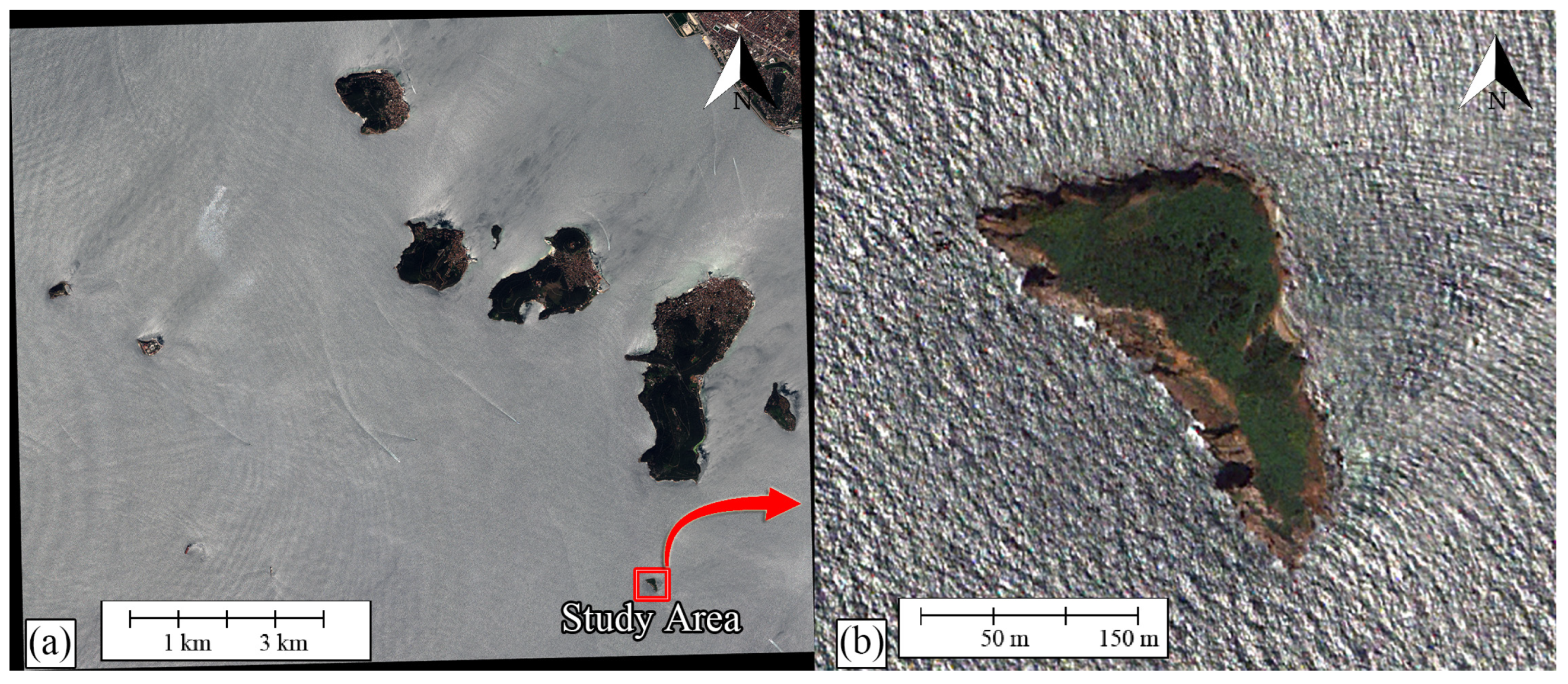
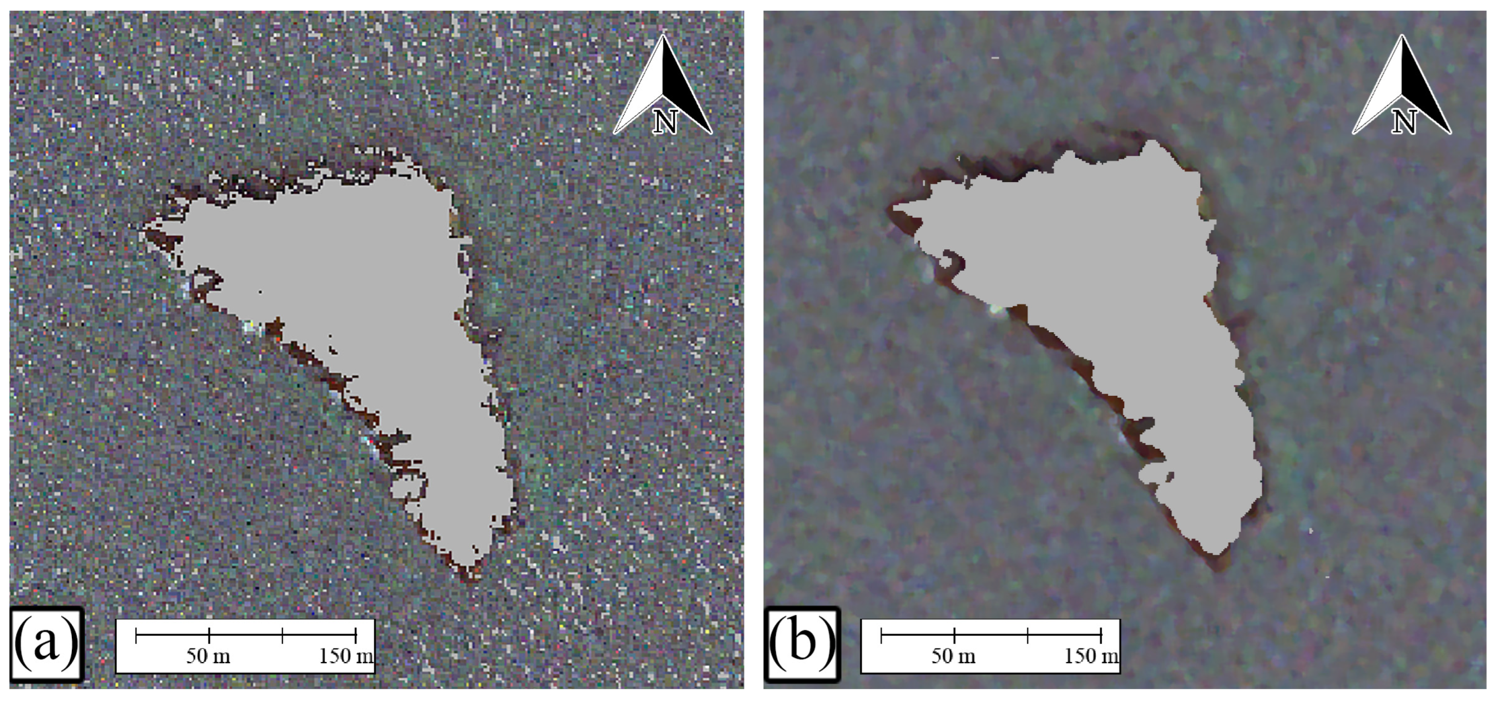
2.1. Study Area
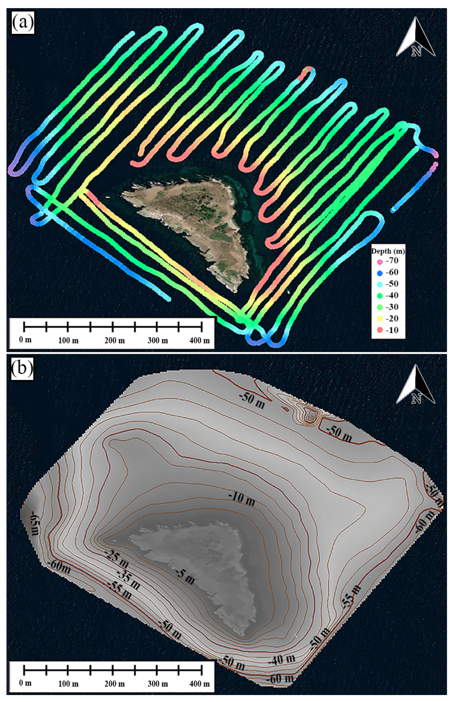
2.2. In Situ Bathymetry Measurements
2.3. WorldView-2 (WV-2) Imagery
2.4. Methodology
2.4.1. Pre-Processing
- i.
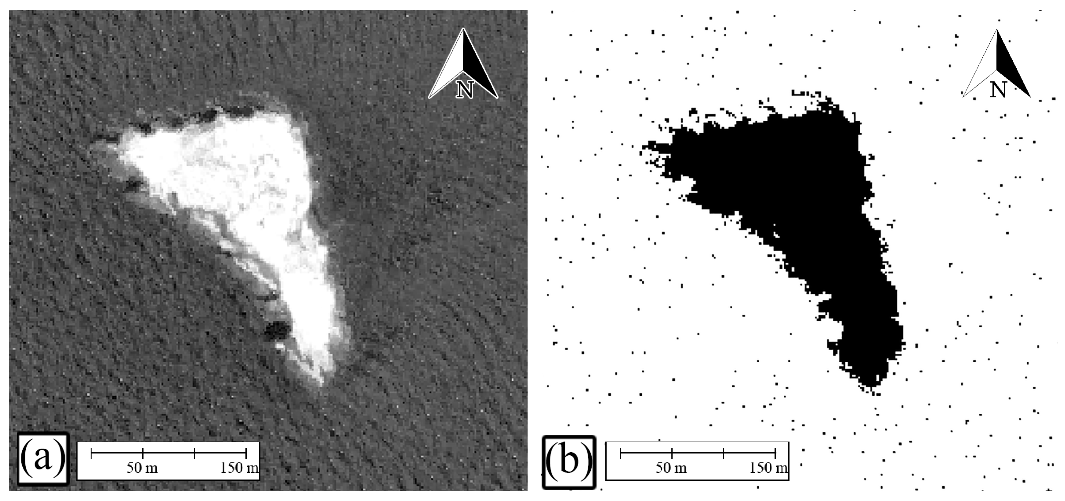
- Water Pixel Extraction and Landmask Creation
- ii.
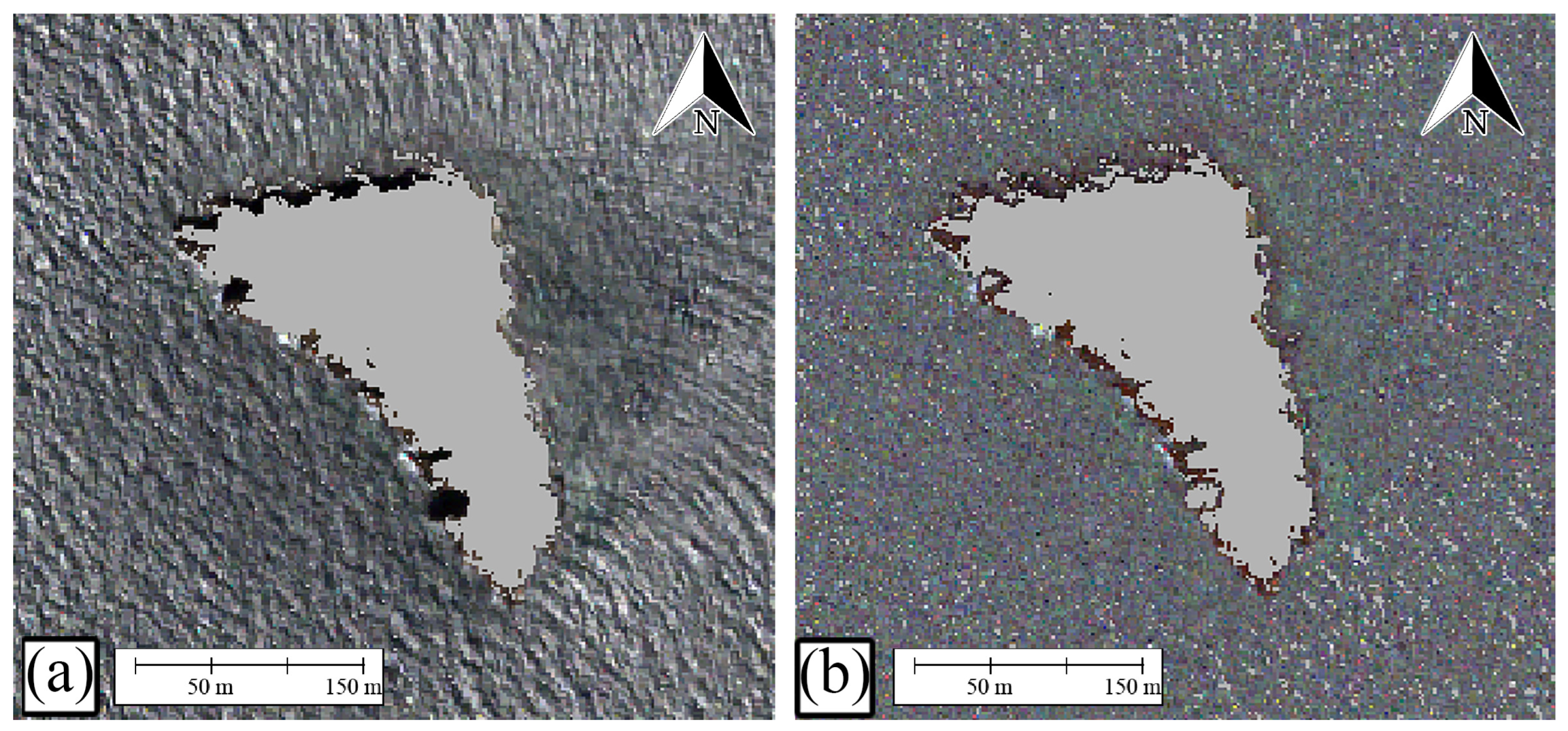
- Sun-glint Correction
- iii.
- Median Filtering:
- iv.
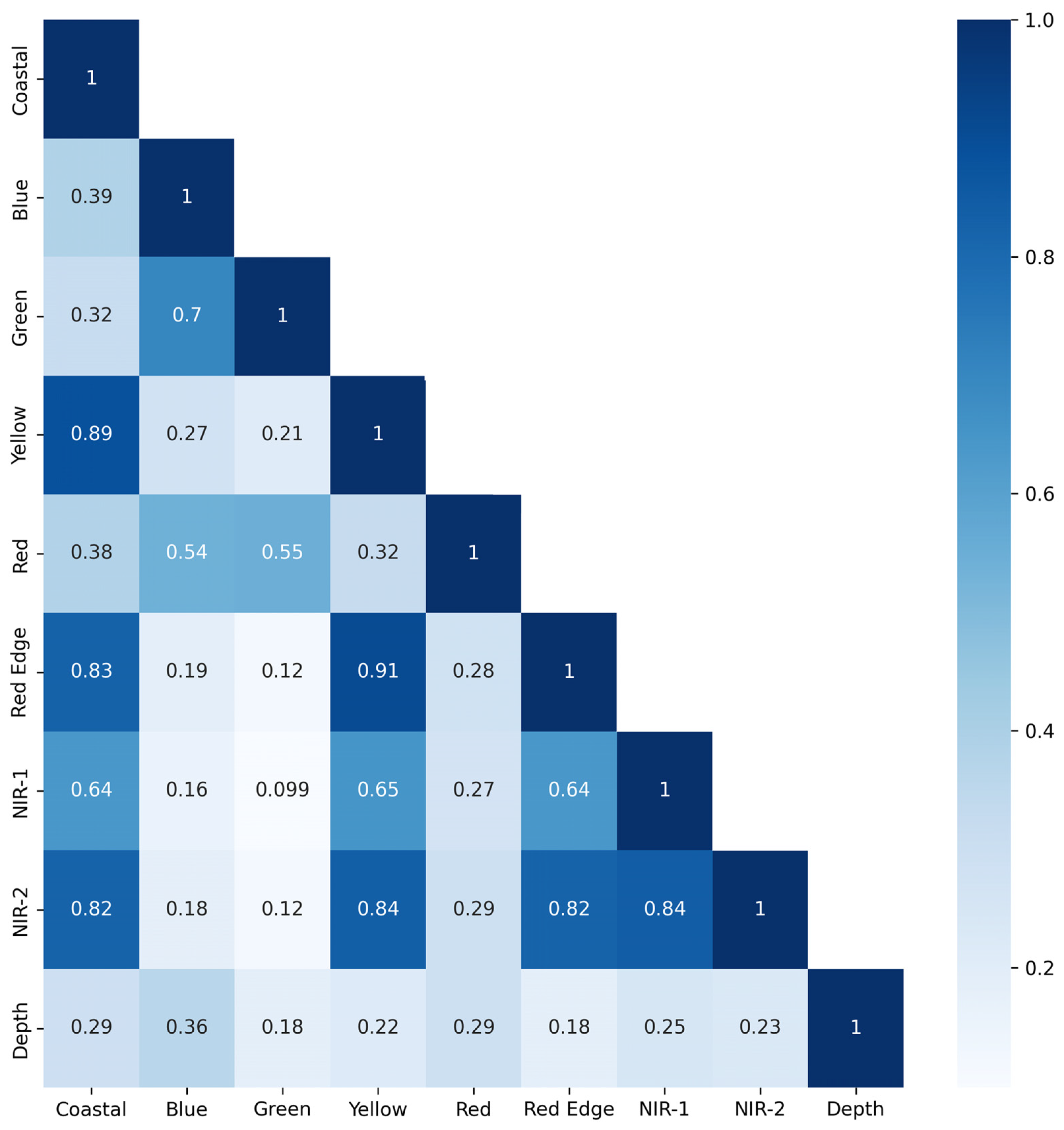
- Dataset Preparation:
2.4.2. Bathymetry Derivation from WV-2 Satellite Imagery
- i.
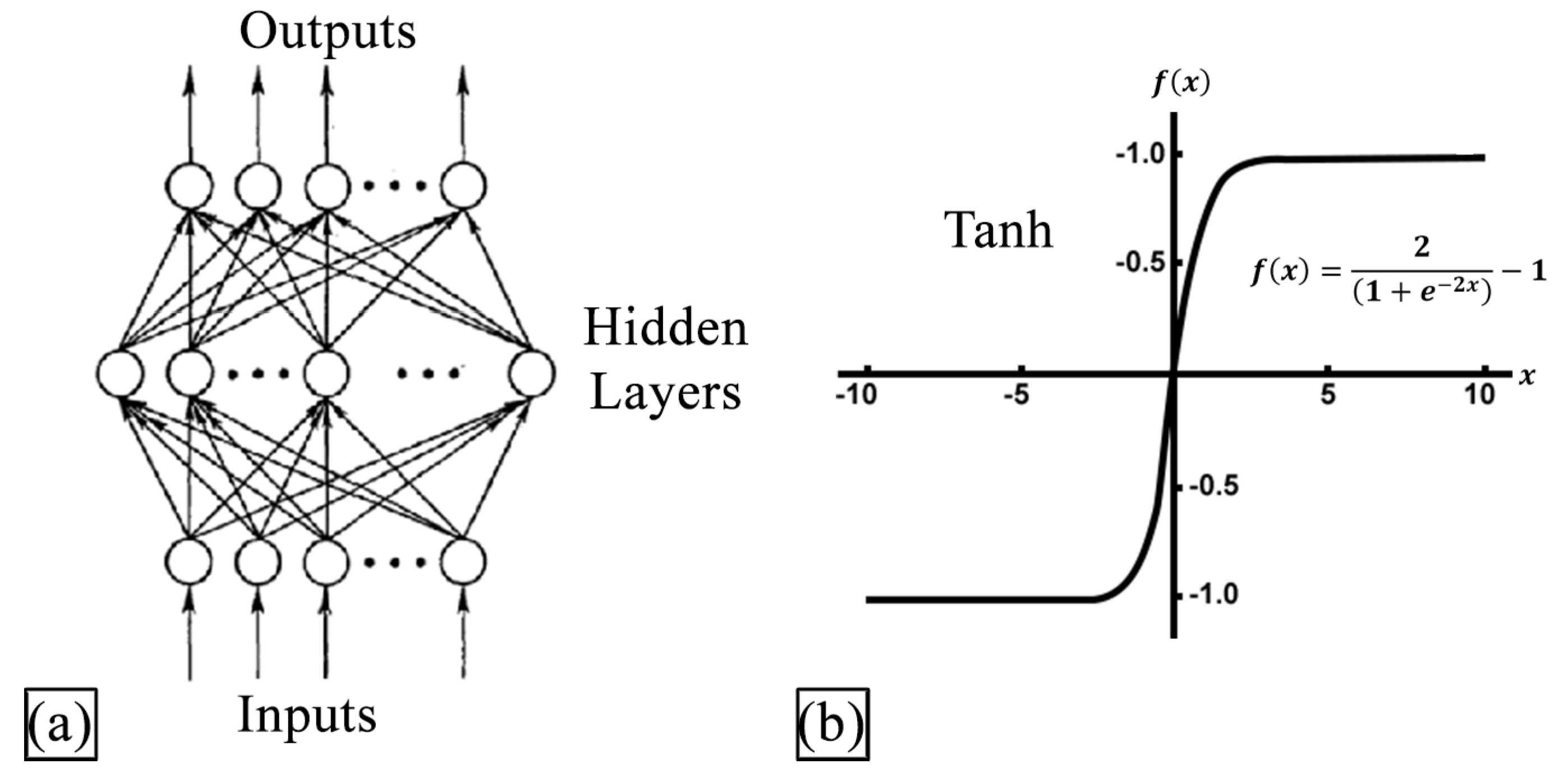
- Multi-Layer Perceptron (MLP) Regression Approach
- ii.
- Random Forest (RF) Regression Approach
2.4.3. Accuracy Assessment
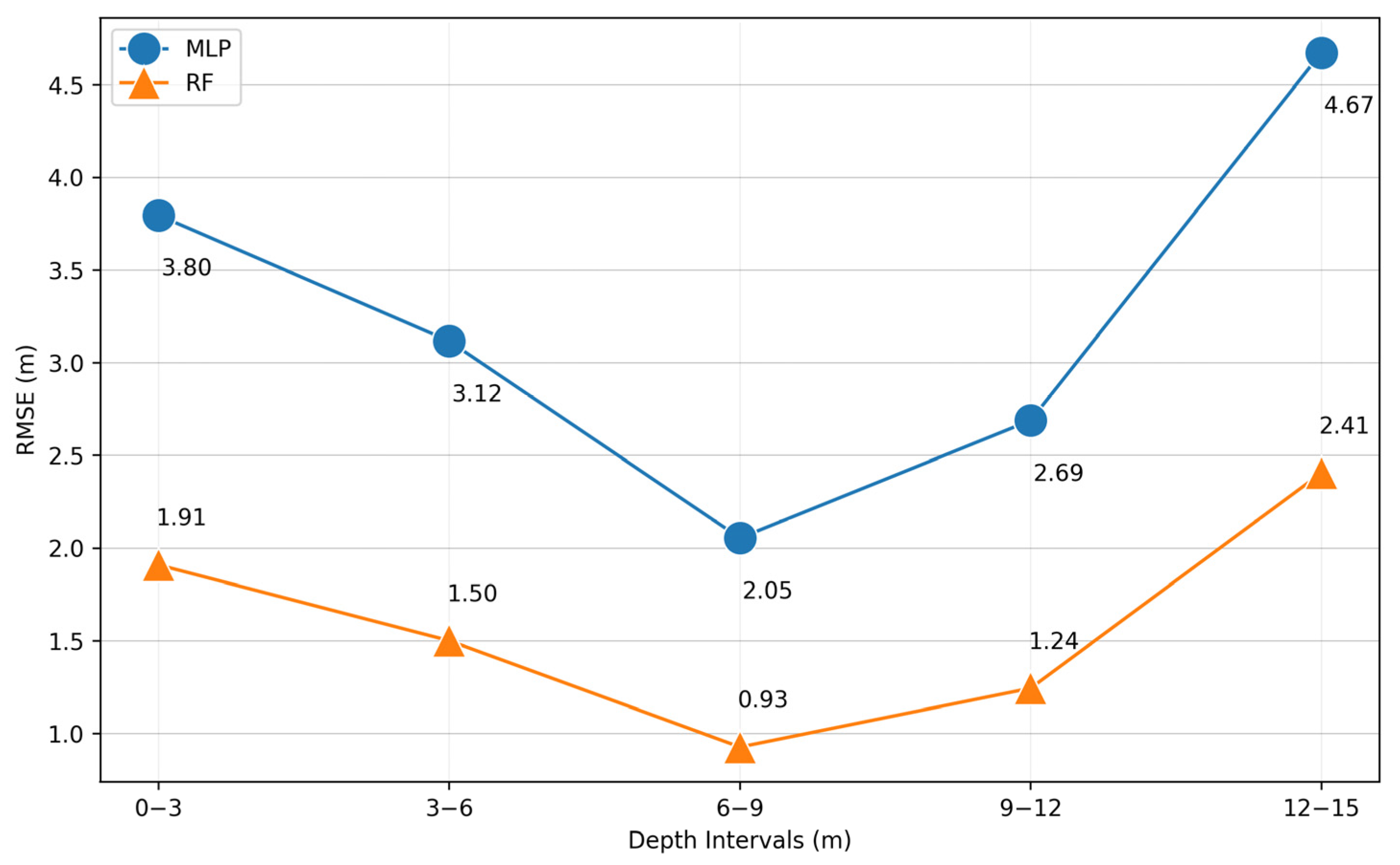
3. Results
4. Conclusions
Author Contributions
Funding
Institutional Review Board Statement
Informed Consent Statement
Acknowledgments
Conflicts of Interest
References
- Casal, G.; Hedley, J.D.; Monteys, X.; Harris, P.; Cahalane, C.; McCarthy, T. Satellite-Derived Bathymetry in Optically Complex Waters Using a Model Inversion Approach and Sentinel-2 Data. Estuar. Coast. Shelf Sci. 2020, 241, 106814. [Google Scholar] [CrossRef]
- Stumpf, R.P.; Holderied, K.; Sinclair, M. Determination of Water Depth with High-Resolution Satellite Imagery over Variable Bottom Types. Limnol. Oceanogr. 2003, 48, 547–556. [Google Scholar] [CrossRef]
- Jawak, S.D.; Vadlamani, S.S.; Luis, A.J. A Synoptic Review on Deriving Bathymetry Information Using Remote Sensing Technologies: Models, Methods and Comparisons. Adv. Remote Sens. 2015, 4, 147. [Google Scholar] [CrossRef]
- Poursanidis, D.; Traganos, D.; Reinartz, P.; Chrysoulakis, N. On the Use of Sentinel-2 for Coastal Habitat Mapping and Satellite-Derived Bathymetry Estimation Using Downscaled Coastal Aerosol Band. Int. J. Appl. Earth Obs. Geoinf. 2019, 80, 58–70. [Google Scholar] [CrossRef]
- Muzirafuti, A.; Crupi, A.; Lanza, S.; Barreca, G.; Randazzo, G. Shallow Water Bathymetry by Satellite Image: A Case Study on the Coast of San Vito Lo Capo Peninsula, Northwestern Sicily, Italy. In Proceedings of the IMEKO TC-19 International Workshop on Metrology for the Sea, Genoa, Italy, 3–5 October 2019; pp. 3–5. [Google Scholar]
- Li, J.; Knapp, D.E.; Schill, S.R.; Roelfsema, C.; Phinn, S.; Silman, M.; Mascaro, J.; Asner, G.P. Adaptive Bathymetry Estimation for Shallow Coastal Waters Using Planet Dove Satellites. Remote Sens. Environ. 2019, 232, 111302. [Google Scholar] [CrossRef]
- Ashphaq, M.; Srivastava, P.K.; Mitra, D. Review of Near-Shore Satellite Derived Bathymetry: Classification and Account of Five Decades of Coastal Bathymetry Research. J. Ocean Eng. Sci. 2021, 6, 340–359. [Google Scholar]
- Douglas, B.C.; Cheney, R.E. Geosat: Beginning a New Era in Satellite Oceanography. J. Geophys. Res. Ocean. 1990, 95, 2833–2836. [Google Scholar] [CrossRef]
- Eugenio, F.; Martin, J.; Marcello, J.; Bermejo, J.A. Worldview-2 High Resolution Remote Sensing Image Processing for the Monitoring of Coastal Areas. In Proceedings of the 21st European Signal Processing Conference (EUSIPCO 2013), Marrakech, Morocco, 9–13 September 2013; IEEE: Piscataway, NJ, USA, 2013; pp. 1–5. [Google Scholar]
- Evagorou, E.; Argyriou, A.; Papadopoulos, N.; Mettas, C.; Alexandrakis, G.; Hadjimitsis, D. Evaluation of Satellite-Derived Bathymetry from High and Medium-Resolution Sensors Using Empirical Methods. Remote Sens. 2022, 14, 772. [Google Scholar] [CrossRef]
- Alevizos, E. A Combined Machine Learning and Residual Analysis Approach for Improved Retrieval of Shallow Bathymetry from Hyperspectral Imagery and Sparse Ground Truth Data. Remote Sens. 2020, 12, 3489. [Google Scholar] [CrossRef]
- Dickens, K.; Armstrong, A. Application of Machine Learning in Satellite Derived Bathymetry and Coastline Detection. SMU Data Sci. Rev. 2019, 2, 4. [Google Scholar]
- Darmanin, G.; Gauci, A.; Deidun, A.; Galone, L.; D’Amico, S. Satellite-Derived Bathymetry for Selected Shallow Maltese Coastal Zones. Appl. Sci. 2023, 13, 5238. [Google Scholar] [CrossRef]
- Zhong, J.; Sun, J.; Lai, Z.; Song, Y. Nearshore Bathymetry from ICESat-2 LiDAR and Sentinel-2 Imagery Datasets Using Deep Learning Approach. Remote Sens. 2022, 14, 4229. [Google Scholar] [CrossRef]
- Xie, C.; Chen, P.; Zhang, Z.; Pan, D. Satellite-Derived Bathymetry Combined with Sentinel-2 and ICESat-2 Datasets Using Machine Learning. Front. Earth Sci. 2023, 11, 1111817. [Google Scholar] [CrossRef]
- Duan, Z.; Chu, S.; Cheng, L.; Ji, C.; Li, M.; Shen, W. Satellite-Derived Bathymetry Using Landsat-8 and Sentinel-2A Images: Assessment of Atmospheric Correction Algorithms and Depth Derivation Models in Shallow Waters. Opt. Express 2022, 30, 3238–3261. [Google Scholar] [CrossRef] [PubMed]
- Sagawa, T.; Yamashita, Y.; Okumura, T.; Yamanokuchi, T. Satellite Derived Bathymetry Using Machine Learning and Multi-Temporal Satellite Images. Remote Sens. 2019, 11, 1155. [Google Scholar] [CrossRef]
- Tonion, F.; Pirotti, F.; Faina, G.; Paltrinieri, D. A Machine Learning Approach to Multispectral Satellite Derived Bathymetry. ISPRS Ann. Photogramm. Remote Sens. Spat. Inf. Sci. 2020, 3, 565–570. [Google Scholar] [CrossRef]
- Liu, S.; Gao, Y.; Zheng, W.; Li, X. Performance of Two Neural Network Models in Bathymetry. Remote Sens. Lett. 2015, 6, 321–330. [Google Scholar] [CrossRef]
- Hakim, L.; Lazuardi, W.; Astuty, I.S.; Al Hadi, A.; Hermayani, R.; Noviandias, D.; Dewi, A.C. Assessing Worldview-2 Satellite Imagery Accuracy for Bathymetry Mapping in Pahawang Island, Lampung, Indonesia. IOP Conf. Ser. Earth Environ. Sci. 2018, 165, 012027. [Google Scholar] [CrossRef]
- Deidda, M.; Sanna, G. Bathymetric Extraction Using WorldView-2 High Resolution Images. Int. Arch. Photogramm. Remote Sens. Spat. Inf. Sci. 2012, 39, 153–157. [Google Scholar] [CrossRef]
- Cao, B.; Fang, Y.; Jiang, Z.; Gao, L.; Hu, H. Shallow Water Bathymetry from WorldView-2 Stereo Imagery Using Two-Media Photogrammetry. Eur. J. Remote Sens. 2019, 52, 506–521. [Google Scholar] [CrossRef]
- Manessa, M.D.M.; Kanno, A.; Sekine, M.; Haidar, M.; Yamamoto, K.; Imai, T.; Higuchi, T. Satellite-Derived Bathymetry Using Random Forest Algorithm and Worldview-2 Imagery. Geoplanning J. Geomat. Plan. 2016, 3, 117. [Google Scholar] [CrossRef]
- Knudby, A.; Richardson, G. Incorporation of Neighborhood Information Improves Performance of SDB Models. Remote Sens. Appl. Soc. Environ. 2023, 32, 101033. [Google Scholar] [CrossRef]
- Zhou, W.; Tang, Y.; Jing, W.; Li, Y.; Yang, J.; Deng, Y.; Zhang, Y. A Comparison of Machine Learning and Empirical Approaches for Deriving Bathymetry from Multispectral Imagery. Remote Sens. 2023, 15, 393. [Google Scholar] [CrossRef]
- Taşkın, E.; Tsiamis, K.; Orfanidis, S. Ecological Quality of the Sea of Marmara (Turkey) Assessed by the Marine Floristic Ecological Index (MARFEI). J. Black Sea/Mediterr. Environ. 2018, 24, 97–114. [Google Scholar]
- Topaloğlu, B. Sponges of the Sea of Marmara with a New Record for Turkish Sponge Fauna. In The Sea of Marmara Marine Biodiversity, Fisheries, Conservation and Governance; Özsoy, E., Çağatay, M.N., Balkıs, N., Balkıs, N., Öztürk, B., Eds.; Turkish Marine Research Foundation: İstanbul, Turkey, 2016; pp. 418–427. [Google Scholar]
- Topçu, N.E.; Yılmaz, I.N.; Saraçoğlu, C.; Barraud, T.; Öztürk, B. Size Matters When It Comes to the Survival of Transplanted Yellow Gorgonian Fragments. J. Nat. Conserv. 2023, 71, 126326. [Google Scholar] [CrossRef]
- Reson Inc. Navisound 600RT Series; Reson Inc.: Ventura, CA, USA, 2006. [Google Scholar]
- TUDES Portal. Available online: https://tudes.harita.gov.tr/ (accessed on 15 June 2023).
- Boissonnat, J.-D.; Cazals, F. Smooth Surface Reconstruction via Natural Neighbour Interpolation of Distance Functions. In Proceedings of the Sixteenth Annual Symposium on Computational Geometry, Hong Kong, China, 12–14 June 2000; pp. 223–232. [Google Scholar]
- Sibson, R. A Brief Description of Natural Neighbour Interpolation. In Interpreting Multivariate Data; John Wiley & Sons: New York, NY, USA, 1981; pp. 21–36. [Google Scholar]
- DigitalGlobe. Accuracy of Worldview Products. Available online: https://dg-cms-uploads-production.s3.amazonaws.com/uploads/document/file/38/DG_ACCURACY_WP_V3.pdf (accessed on 12 September 2020).
- Basith, A.; Prastyani, R. Evaluating ACOMP, FLAASH and QUAC on Worldview-3 for Satellite Derived Bathymetry (SDB) in Shallow Water. Geod. Cartogr. 2020, 46, 151–158. [Google Scholar] [CrossRef]
- Dierssen, H.M.; Garaba, S.P. Bright Oceans: Spectral Differentiation of Whitecaps, Sea Ice, Plastics, and Other Flotsam. Recent Adv. Study Ocean. Whitecaps Twixt Wind Waves 2020, 197–208. [Google Scholar]
- Gao, B.-C. NDWI—A Normalized Difference Water Index for Remote Sensing of Vegetation Liquid Water from Space. Remote Sens. Environ. 1996, 58, 257–266. [Google Scholar] [CrossRef]
- Hedley, J.D.; Harborne, A.R.; Mumby, P.J. Simple and Robust Removal of Sun Glint for Mapping Shallow-Water Benthos. Int. J. Remote Sens. 2005, 26, 2107–2112. [Google Scholar] [CrossRef]
- Doxani, G.; Papadopoulou, M.; Lafazani, P.; Pikridas, C.; Tsakiri-Strati, M. Shallow-Water Bathymetry over Variable Bottom Types Using Multispectral Worldview-2 Image. Int. Arch. Photogramm. Remote Sens. Spat. Inf. Sci. 2012, 39, 159–164. [Google Scholar] [CrossRef]
- Hall, M.A. Correlation-Based Feature Selection for Machine Learning. Ph.D. Thesis, The University of Waikato, Hamilton, New Zealand, 1999. [Google Scholar]
- Vagizov, M.; Potapov, A.; Konzhgoladze, K.; Stepanov, S.; Martyn, I. Prepare and Analyze Taxation Data Using the Python Pandas Library. IOP Conf. Ser. Earth Environ. Sci. 2021, 876, 012078. [Google Scholar] [CrossRef]
- Borkin, D.; Némethová, A.; Michal’čonok, G.; Maiorov, K. Impact of Data Normalization on Classification Model Accuracy. Res. Pap. Fac. Mater. Sci. Technol. Slovak Univ. Technol. 2019, 27, 79–84. [Google Scholar] [CrossRef]
- Nawi, N.M.; Atomi, W.H.; Rehman, M.Z. The Effect of Data Pre-Processing on Optimized Training of Artificial Neural Networks. Procedia Technol. 2013, 11, 32–39. [Google Scholar] [CrossRef]
- Murtagh, F. Multilayer Perceptrons for Classification and Regression. Neurocomputing 1991, 2, 183–197. [Google Scholar] [CrossRef]
- Manaf, S.A.; Mustapha, N.; Sulaiman, M.; Husin, N.A.; Hamid, M.R.A. Artificial Neural Networks for Satellite Image Classification of Shoreline Extraction for Land and Water Classes of the North West Coast of Peninsular Malaysia. Adv. Sci. Lett. 2018, 24, 1382–1387. [Google Scholar] [CrossRef]
- Sharma, S. Activation Functions in Neural Networks. Towards Data Science, 6 September 2017. [Google Scholar]
- Wang, Y.; Zhou, X.; Li, C.; Chen, Y.; Yang, L. Bathymetry Model Based on Spectral and Spatial Multifeatures of Remote Sensing Image. IEEE Geosci. Remote Sens. Lett. 2019, 17, 37–41. [Google Scholar] [CrossRef]
- Buitinck, L.; Louppe, G.; Blondel, M.; Pedregosa, F.; Mueller, A.; Grisel, O.; Niculae, V.; Prettenhofer, P.; Gramfort, A.; Grobler, J.; et al. API Design for Machine Learning Software: Experiences from the Scikit-Learn Project. In Proceedings of the ECML PKDD Workshop: Languages for Data Mining and Machine Learning, Prague, Czech Republic, 23–27 September 2013; pp. 108–122. [Google Scholar]
- Saputro, D.R.S.; Widyaningsih, P. Limited Memory Broyden-Fletcher-Goldfarb-Shanno (L-BFGS) Method for the Parameter Estimation on Geographically Weighted Ordinal Logistic Regression Model (GWOLR). In Proceedings of the AIP Conference Proceedings, Yogyakarta, Indonesia, 15–16 May 2017; AIP Publishing LLC: Melville, NY, USA, 2017; Volume 1868, p. 040009. [Google Scholar]
- Breiman, L. Random Forests. Mach. Learn. 2001, 45, 5–32. [Google Scholar] [CrossRef]


Disclaimer/Publisher’s Note: The statements, opinions and data contained in all publications are solely those of the individual author(s) and contributor(s) and not of MDPI and/or the editor(s). MDPI and/or the editor(s) disclaim responsibility for any injury to people or property resulting from any ideas, methods, instructions or products referred to in the content. |
© 2023 by the authors. Licensee MDPI, Basel, Switzerland. This article is an open access article distributed under the terms and conditions of the Creative Commons Attribution (CC BY) license (https://creativecommons.org/licenses/by/4.0/).
Share and Cite
Çelik, O.İ.; Büyüksalih, G.; Gazioğlu, C. Improving the Accuracy of Satellite-Derived Bathymetry Using Multi-Layer Perceptron and Random Forest Regression Methods: A Case Study of Tavşan Island. J. Mar. Sci. Eng. 2023, 11, 2090. https://doi.org/10.3390/jmse11112090
Çelik Oİ, Büyüksalih G, Gazioğlu C. Improving the Accuracy of Satellite-Derived Bathymetry Using Multi-Layer Perceptron and Random Forest Regression Methods: A Case Study of Tavşan Island. Journal of Marine Science and Engineering. 2023; 11(11):2090. https://doi.org/10.3390/jmse11112090
Chicago/Turabian StyleÇelik, Osman İsa, Gürcan Büyüksalih, and Cem Gazioğlu. 2023. "Improving the Accuracy of Satellite-Derived Bathymetry Using Multi-Layer Perceptron and Random Forest Regression Methods: A Case Study of Tavşan Island" Journal of Marine Science and Engineering 11, no. 11: 2090. https://doi.org/10.3390/jmse11112090
APA StyleÇelik, O. İ., Büyüksalih, G., & Gazioğlu, C. (2023). Improving the Accuracy of Satellite-Derived Bathymetry Using Multi-Layer Perceptron and Random Forest Regression Methods: A Case Study of Tavşan Island. Journal of Marine Science and Engineering, 11(11), 2090. https://doi.org/10.3390/jmse11112090