Application of the Most Sensitive Initial Error in Sampling Scheme Design for a Mobile Platform

Abstract

Since ocean mobile observation equipment and numerical models have achieved remarkable results, the combination of the two has become an influential topic. A numerical model provides auxiliary information for the arrangement of observation equipment. As feedback, observations help produce more accurate initial conditions when incorporated into data assimilation. However, it is still worth investigating the ways to select the most valuable observation sites within the computational domain and the ways to design the observation scheme of the mobile platform. To improve the efficiency of observation, researchers attempt to select the best observation region in the vast ocean. The approach of deploying additional observing assets in selected regions is referred to as targeted observation. By combining the features of the targeted observation and the mobile observing platform, we propose a design approach for the observation scheme. First, based on a model, we estimate the initial perturbation that causes the greatest change in the sea surface temperature in the future. Then, according to the spatial component of the perturbation, we divide the experimental regions into sensitive regions and non-sensitive regions. Observing system simulation experiments are carried out to verify that samples in sensitive regions are more helpful to improve model prediction. Afterward, considering the variation of the perturbation with time, we propose a hybrid sampling scheme design method for an underwater unmanned vehicle combining Q-learning and particle swarm optimization algorithm. Finally, the effectiveness of the hybrid algorithm is verified by comparing the sampling schemes designed in static environment. This approach provides a dynamic basis for the path planning of mobile observing platforms.

1. Introduction

Coupled models usually suffer from unavoidable errors due to biased initial conditions and parameter schemes [1]. These discrepancies continue to develop and subsequently lead to poor forecast quality [2]. Assimilating observations is helpful for correcting biases in the initial conditions. However, how to deploy the limited observational resources in the vast oceanic space is a question worth investigating. Targeted observation is a technique that deploys additional observing assets in certain key regions to better predict an event at a later time [3]. The key regions are defined as sensitive regions, and are obtained by computing the perturbation that causes the largest change in the ocean state at the time of the event using a numerical model. The idea of targeted observation is similar to that of adaptive sampling [4]. The similarity between targeted observation and adaptive sampling is that both improve the efficiency of observations by selecting optimal observation locations. The difference between them is that adaptive sampling additionally plans the path of the mobile platform. The conditional nonlinear optimal perturbation (CNOP) [5] shows great potential in the process of estimating the value of observations to design a sampling scheme. It refers to the initial perturbation under the constraint that causes the largest increase at a given time and has been applied to targeted observation related to the El Niño-Southern Oscillation [6].

An integrated modeling observation system involves the combination of three subsystems or algorithms [7]: (1) a prediction model that provides supplementary information for scheme design; (2) an optimization algorithm for generating observation schemes; (3) observation platforms with attribute information. Earlier studies focused more on specific fields. Targeted observation is primarily concerned with the location of the deployment of the observing assets. In a related work, Zhou et al., 2022 studied the effect of the spatial structure of the CNOP on the prediction of the Antarctic circulation and demonstrated that it can be used to design an observation network for the Drake Passage [8]. Yang et al., 2020 employed intelligent optimization algorithms with a dimensionality reduction module to compute CNOP in the GFDL CM2p1 model, suggesting that the method is effective for calculating CNOP in complex models [9]. The above studies show that CNOP has great potential for marine science. The design of observation schemes for mobile platforms focuses more on optimization algorithms. Recently, Zeng et al., 2023 presented a novel rapidly exploring tree algorithm for adaptive sampling missions in a three-dimensional environment. They focused on the path planning algorithm, so the sampling goal was to find areas with high temperature/salinity values [10]. Li et al., 2023 proposed a motion planning algorithm for autonomous underwater vehicle (AUV) based on reinforcement learning which incorporates real-time ocean current data into an environmental model to balance realism and complexity [11]. The above research shows that the mobile platform is playing an increasingly vital role in marine engineering. Using the prior information of marine environment to plan the platform path has also become a research hotspot.

Despite previous research demonstrating that targeted observations can increase sample efficiency, several significant concerns remain. One of the most challenging problems is the design of an observation scheme based on the estimated region sensitivity information. After all, the observation task depends on the platform to be completed, and a better observation scheme can significantly increase efficiency. While algorithms for planning global observation paths are becoming more sophisticated, scientific evaluation of observation locations remains a problem. In the early stage, Lermusiaux 2007 proposed the combination of a numerical model and an observation scheme to reduce the blindness. This work focused on regions of great uncertainties (estimated by the error subspace statistical estimation) [4]. Lately, in combination with the CNOP method, Liu et al., 2021 designed Z-shape observation stations based on time-varying sensitive regions [12]. To achieve the objective of improving the observation efficiency of mobile platforms, we try to combine the excellent work in the field of targeted observation with observation path planning. For mobile platforms, we refer to existing large underwater unmanned vehicles [13] that can sail for days to perform sampling missions. When the spatial resolution of the numerical model is higher, the forecast of the marine environment is more detailed, and the scheme of a smaller mobile observation platform can be designed using this method. Employing a time-varying optimal initial error sequence, we design a sampling scheme for a mobile platform and evaluate the effect of sampling according to this scheme on improving prediction.

We apply a simplified air–sea coupled model [14] to verify the concept. The model is simple in principle and has two-dimensional space characteristics, which is suitable for verifying the new method for designing adaptive sampling schemes. We first use the “dimensionality reduction—intelligent algorithm” solution framework to calculate CNOP. The intelligent algorithm part adopts an improved bare-bones particle swarm optimization (BBPSO) [15]. Then, we investigate the effect of the spatial distribution of the CNOP on the sampling in the twin experimental framework constructed by the model we use. An ensemble adjustment Kalman filter (EAKF) [16] is adopted as a data assimilation method to the observing system simulation experiment (OSSE). The experiment is split into two parts: observations are assimilated once and repeatedly at selected locations to simulate different types of platforms. Finally, based on the conclusions drawn in OSSE, we propose an adaptive sampling scheme design approach for mobile platforms. This approach combines the global vision of swarm intelligence optimization with reinforcement learning to provide technical support for practical sampling.

The paper is organized as follows. The experimental environment and methods, including the numerical model we use, EAKF, and the definition and solution method of CNOP, are briefly described in Section 2. In Section 3, based on CNOP, we first partition the experimental region into sensitive and non-sensitive regions by a clustering method. Then, with the aid of EAKF, we examine the sensitive regions in the OSSE. Finally, through the CNOP and the characteristics of the platform, we propose a sampling scheme design approach based on the mobile platform in Section 4. A summary and discussion is described in Section 5.

2. Method

2.1. Experimental Environment

An intermediate coupled circulation model (ICCM) is used to prove the design method of the sampling scheme for a mobile platform combined with targeted observation. “Intermediate” here represents a type of model that is more complex than conceptual models with no physical meaning, simpler than advanced operational models. The ICCM comes from Zhang et al., 2015 [14], which is the combination of the model used by Dommenget and Flöter 2011 [17] and Wu et al., 2012 [18]. It is a two-dimensional model under the premise of simplifying the spatial structure of the subsurface ocean. With its energy-conserving properties and simplicity principle, the ICCM is suitable for preliminary validation of the new approach.

Assuming that the mobile platform travels at an average speed of 2.5 Kn (1 Kn = 1.85 km/h), in 6 h, it travels a distance of 27.75 km, or about ${0.25}^{\circ }$ in latitude and longitude. For the simplified model we use, the spatial resolution does not meet the needs of designing a sampling scheme for a mobile platform. Therefore, it is increased by nesting through the method proposed by Bai et al., 2010 [19] before application. Zhao et al., 2023 [20] describes the details of implementing multi-layer nesting of the ICCM. The nested ICCM with spatial resolution of ${0.1}^{\circ }$ and a model time step of 12 h can support our research.

There are three reasons for choosing the nested ICCM to provide forecast information: (1) compared with the ideal conceptual model, this model has physical meaning and two-dimensional spatial characteristics, which can be used for the study of sampling scheme design methods; (2) compared with the operational model (such as the regional oceanic modeling system [21]), this model simplifies a lot of physical processes, which is suitable for the verification of new methods; (3) due to the limitation of the computing and navigation capability of the mobile platform, nesting models are often needed in the study of sampling scheme design, and they can meet the research needs in the initial stage. Our research focuses on the method for designing sampling schemes for a marine mobile platform. The atmospheric temperature, land temperature and other variables simulated cannot meet the research needs. In addition, the ICCM lacks three-dimensional spatial structure, and the simulation of ocean surface temperature is not accurate enough. Therefore, we choose the sea surface temperature (SST) as the research target in this paper. The SST is a two-dimensional environment variable, which is suitable for method verification in a two-dimensional environment. Although this variable can be obtained by remote sensing over a wide scale, it does not affect our study of the observation path of the mobile platform. In a follow-up study, we will try more complex operational ocean models (for instance, HYCOM [22] or NEMO [23]) and investigate variables such as underwater temperature, salinity or density to extend the problem to three dimensions.

The dynamics equation related to SST in nested ICCM is described in Equation (1):

$$\partial T_s/\partial t+u_s·\nabla T_s-K_h\phi =1/{\gamma }_s·\left(F_{So}+F_{th}+F_l+F_s+F_o+F_C\right)+{\kappa }_s{\nabla }^2{T}_s,$$

(1)

where $T_s$ is the SST whose horizontal diffusivity coefficient is denoted by ${\kappa }_s$. $K_h$ denotes the strength of upwelling, and $u_s$ represents the oceanic current field. ${\gamma }_s$ represents the oceanic heat capacity, and $\phi$ is the oceanic stream. The heat flux terms included the absorbed incoming solar ($F_{So}$), the net thermal radiation ($F_{th}$), the latent heat released into the surface layer ($F_l$), the sensible heat flux ($F_s$), the net heat flux between the upper and deeper ocean ($F_o$) and the empirical flux correction term ($F_C$). Details about other components and parameterization schemes are described in Zhang et al., 2015 [14]. Zhao et al., 2019 provides a parameter estimation method and a method to construct the twin experiment framework for OSSE based on the ICCM [2]. The main difference between perfect and biased experimental frameworks is the simulation of outgoing planetary longwave radiation. The perfect experimental framework uses the physical parameterization scheme in Dommenget and Flöter 2011 [17], and the biased experimental framework uses the scheme in Thompson and Warren 1982 [24]. The twinning experimental framework in OSSE is shown in Figure 1.

The perfect and biased experimental frameworks are used for simulating forecasts and truth, respectively. The observations, truth and forecasts mentioned in this paper are all simulation results. Although the perfect and biased experimental frameworks adopt different parameterization schemes, both are constructed by ICCM, so the forecast error in this paper is not large. Observations are generated by adding a random error with standard deviation $0.1$ K to the truth. The error is intended to match the forecast error in our simulation.

Considering the sailing ability of the mobile platform at a certain speed, the experiment time is set to 4 days in this paper. Thus, the predictions we use are short-term. To ensure the robustness of the experimental results in different experimental regions and times, we set up four experiments. To rule out topographical factors, two regions are selected, one without land (129${}^{\circ }$ E∼134${}^{\circ }$ E, 21${}^{\circ }$ N∼26${}^{\circ }$ N) and one with land (121${}^{\circ }$ E∼126${}^{\circ }$ E, 19${}^{\circ }$ N∼24${}^{\circ }$ N). The sampling times are chosen to be 1–4 April and 1–4 October, which reduces the effect of seasonal factors. For convenience, Experimental scenarios 1, 2, 3, and 4 are abbreviated as EX1, EX2, EX3, and EX4, respectively. Figure 2 shows the topography of the experimental regions and the reference states for the four experiments. The time and place settings in four experiments are described in

Table 1. The setup of the location, time in four experiments.

Serial Number	Experimental Region	Experimental Time
EX1	(129${}^{\circ }$ E∼134${}^{\circ }$ E, 21${}^{\circ }$ N∼26${}^{\circ }$ N)	April 1 to 4
EX2	(129${}^{\circ }$ E∼134${}^{\circ }$ E, 21${}^{\circ }$ N∼26${}^{\circ }$ N)	October 1 to 4
EX3	(121${}^{\circ }$ E∼126${}^{\circ }$ E, 19${}^{\circ }$ N∼24${}^{\circ }$ N)	April 1 to 4
EX4	(121${}^{\circ }$ E∼126${}^{\circ }$ E, 19${}^{\circ }$ N∼24${}^{\circ }$ N)	October 1 to 4

.

2.2. Observation Sensitivity Estimation

EAKFs estimate the deviation of the forecast $\Delta Z_{i,j}$ through Equation (2).

$$\Delta Z_{i,j}=\frac{Cov\left(Z_j,Y_k\right)}{{\left({\sigma }_{k,k}^p\right)}^2}·\left[\frac{{\left({\sigma }_{k,k}^p\right)}^2}{{\left({\sigma }_y^o\right)}^2+{\left({\sigma }_{k,k}^p\right)}^2}\left(Y^o-{\overline{Y}}_k^p\right)+\left(\sqrt{\frac{{\left({\sigma }_y^o\right)}^2}{{\left({\sigma }_y^o\right)}^2+{\left({\sigma }_{k,k}^p\right)}^2}}-1\right)\left(Y_{k,i}^p-{\overline{Y}}_k^p\right)\right].$$

(2)

Subscripts i, j, k represent the index of the ensemble member, the grid point, and the observation, respectively. $Z_j$ denotes an ensemble background state. $Y_k$ is a single valid observation at location k, whose value and standard deviation are $Y_k^o$ and ${\sigma }_y^o$, respectively. ${\overline{Y}}_k^p$ and ${\sigma }_{k,k}^p$ represent the ensemble mean and standard deviation of the prediction. The detailed derivation of the formula is shown in Zhao et al., 2019 [2], and only the conclusions are utilized in this paper.

The spatial distribution of CNOP is used to estimate the most sensitive observation locations. We assume that the original output of the nested ICCM is $M_t\left(X_0\right)$ after integrating over time t, when the initial temperature $X_0$ is input. After adding a small perturbation $x_0$ to the initial state $X_0$, its output becomes $M_t(X_0+x_0)$. The CNOP $x_{0\delta }$ is calculated as

$$\begin{array}{c}{x}_{0\delta }=\underset{∥x_0∥\le \delta }{\arg max}∥M_t(X_0+x_0)-M_t\left(X_0\right)∥\end{array},$$

(3)

where $∥·∥$ is the 2-norm, and $∥M_t(X_0+x_0)-M_t\left(X_0\right)∥$ means the objective function for calculating the CNOP. In this problem, it is the 2-norm of the SST change at time t caused by the initial perturbation $x_0$. $∥x_0∥\le \delta$ represents the constraint on the perturbation, which avoids the phenomenon that the objective function increases with the norm of initial perturbation.

The choice of condition $\delta$ is the next problem. We refer to the method of Yang et al., 2020 [9], and combine the features of ensemble predictions. The maximum deviation of each ensemble member from the ensemble mean is defined as $\delta$, which is described as

$$\delta =\underset{i\in \left[1,N_E\right]}{max}\left({\sum }_j\sqrt{\Delta T{{}_s^{i,j}}^2}\right),$$

(4)

where $N_E$ denotes the number of ensemble members. $\Delta T{}_s^{i,j}$ represents the deviation from the ensemble mean of the ith ensemble member in location j at the moment adding perturbation. In this way, the problem of defining $\delta$ then becomes the problem of generating a reliable ensemble. The $\delta$ values in the four experiments are 710.3, 522.0, 532.5, 544.6, respectively. Since our problem is to design a sampling scheme for a mobile platform based on the most sensitive initial perturbation, the details of the forecast section were described in Zhao et al., 2019 [2].

Intelligent algorithms, which have the advantage of being simple in principle and do not require adjoint models, have been widely used in the solution process of CNOP [25,26]. Here, we compute the CNOP using a modified version of the bare-bones particle swarm optimization (BBPSO) [27,28] algorithm. The BBPSO was developed from the standard particle swarm optimization algorithm, which has been used in many fields [29]. It simplifies the calculation and reduces human intervention in parameter selection. Feng et al., 2008 proved that this is equivalent to the standard particle swarm optimization [30]. Based on the BBPSO, we tune the parameters by combining the parameter tuning methods in Shi and Eberhart 1998 and Zhang et al., 2014 [31,32]. Equation (5) shows its expression.

$$\begin{array}{c}{X}_{ld}^h=N(\frac{(1-c\left(h\right))P_{ld}^{h-1}+c\left(h\right)P_{gd}^{h-1}}{2},\left|P_{ld}^{h-1}-P_{gd}^{h-1}\right|)\end{array},$$

(5)

where h is the number of iterations, whose maximum is $h_{max}$, and d represents the d-dimensional component of the solution. And l denotes an index of individuals. $X_{ld}^h$ means the d-dimensional component of a solution searched by individual l during iteration h. $P_{ld}^{h-1}$ and $P_{gd}^{h-1}$ mean the d-dimensional component of the optimal solution searched by individual l and the whole population during iteration $h-1$, respectively. When $h=1$, they represent the optimal solution in individual l and the global at the initial time, when the solution space is randomly generated. And $c\left(h\right)$ is a parameter that varies with the number of iterations h, which is essentially the weight of global and local optimal solutions in the process of finding new solutions. We expect it to have a small value early on, thus increasing the search range, and a large value late on, thus accelerating convergence. Therefore, the value of $c\left(h\right)$ is defined as

$$\begin{array}{c}c\left(h\right)=\frac{1}{1+e^{-\frac{h-h_{max}}{2}}};h\in [1,h_{max}]\end{array}.$$

(6)

Although the nested ICCM is smaller than any state-of-the-art numerical earth system model, at a spatial resolution of ${0.1}^{\circ }$, its spatial dimension is still 2601 in the experimental area, which greatly exceeds the optimization capabilities of swarm intelligent optimization algorithms. This also illustrates the necessity of using simplified models in the conceptual stage of engineering problems. To avoid the curse of dimensionality, we reduce the dimensionality before solving CNOP with BBPSO. The calculation procedure is shown in Figure 3. Here, the coupling model is invoked independently several times, as is the transition matrix between higher and lower dimensional spaces.

3. Determination of Sensitive Region

We assume that a period of time is used for the deployment and commissioning of the sampling platform and does not count toward the observing task. Since the temporal resolution of the model is 12 h, the moment we start the task, Day 0.5, is the initial time to add perturbations. The CNOP computed with dimensionality reduction and the BBPSO algorithm is shown in Figure 4.

In the spatial distribution, the dark blue region dominates. The non-dark blue regions in EX1 are in the upper middle and upper right of the region map, and EX2 is in the lower left and middle right. In EX3 and EX4, they are located around land. EX3 is on the upper left and EX4 is on the left.

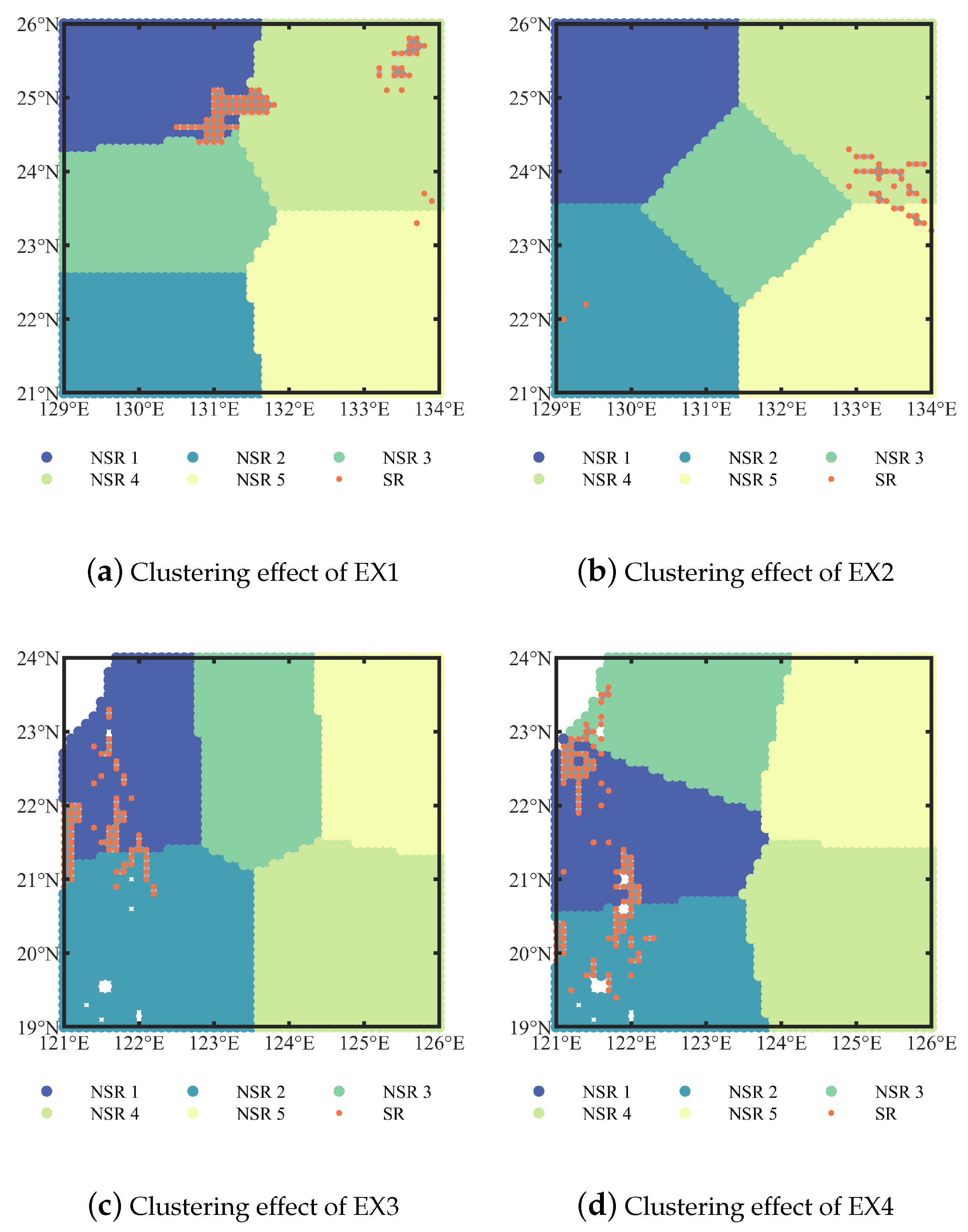
Having obtained the spatial distribution of the CNOP, qualitative characterization of the sensitive regions is the next question to be addressed since the distribution of sensitive areas in the experimental area is not concentrated. To address this issue, we use a k-means algorithm, which clusters data with similar characteristics through unsupervised learning and has been widely used in engineering [33,34]. Regions are clustered into sensitive and non-sensitive regions exactly according to the CNOP. The area of the non-sensitive region is too large compared to the sensitive region, so we divide the non-sensitive region into multiple parts based on spatial location, as in Jiang et al., 2022 [3]. To reduce subjective intervention, we also use the k-means algorithm to complete the division. The partitioning results are shown in Figure 5. For the sake of the legend, we abbreviate the non-sensitive region as 1, the non-sensitive region as 2, the non-sensitive region as 3, the non-sensitive region as 4, the non-sensitive region as 5 and the sensitive region as NSR1, NSR2, NSR3, NSR4, NSR5, and SR in Figure 5.

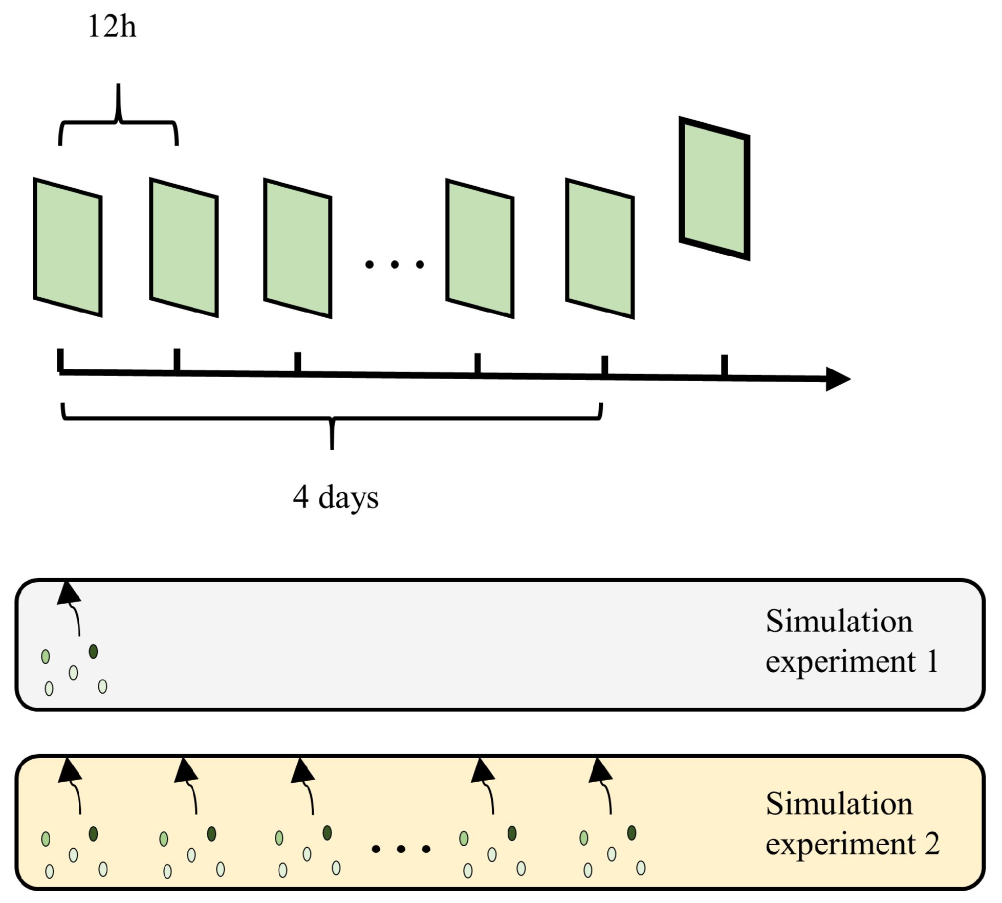
After identifying the sensitive regions, OSSE is used to investigate whether observing samples in the sensitive regions would be more helpful in improving the prediction accuracy on the fourth day. The OSSE is divided into two groups. The experimental setup is shown in Figure 6. The first set is observed only once, when the CNOP is added to simulate the sampling properties of the expendable platform. The second set is observed several times during the sampling period, assimilated once at each step of the model integration, and used to simulate a fixed observing platform. We select five observation sites in each region for OSSE, which are chosen randomly to avoid subjective factors, and this process is performed several times to reduce the chance factor due to the random selection of observation sites.

The first set of experiments is as follows: observations are taken at the initial time when the perturbation is added. The data assimilation module then no longer accepts observations. After four days of observation in the sensitive and non-sensitive regions, we compare the RMSE between the prediction and the truth at the moment corresponding to the reference state. Although there are differences in the parameterization process, the twin experimental framework is derived from the nested ICCM; as a result, the difference between the simulated truth and the prediction is small. Average RMSEs over four days are within $0.45$ K in all four experiments and around $0.3$ K in three of the four experiments. To match the predict error and reduce the influence of observational errors on the experimental results, we set a small observational error as a Gaussian white noise with a mean 0 K and a standard deviation $0.1$ K. The experimental results are shown in Figure 7.

With the exception of EX3, which maintains its RMSE around $0.29$ K, regardless of the observed positional variability, the RMSE obtained by observing in the sensitive region is smaller than the non-sensitive region in the other three experiments. This insensitivity to the observations in EX3 is caused by the low prediction error and fewer observations. Overall, the observations in the sensitive region work better. Existing results suggest that targeted observations in sensitive regions identified through the spatial distribution of the CNOP can indeed help to narrow the observation range and improve the quality of the predictions. But the choice of different observing positions in the same region leads to fluctuations in the results. There are also some cases where observation points selected in the sensitive region are not as good as those in the non-sensitive region (especially in EX4). This suggests that the sensitive region of ocean observations is determined by a variety of factors, and the achievement of a more accurate assessment of the observed values remains an issue worth continuing research for. Moreover, there are two problems with the experimental results presented in Figure 7. The first problem is that the prediction error is relatively small compared to the true situation. There are two reasons for this problem. The first reason is that, in order to simplify the problem, we use a model with a simple structure and parameterization scheme that deviates from the real situation. In the twin framework built on nested ICCM, the simulated prediction error itself is small. The second reason is that, in order to match the predict error and reduce the influence of observational errors, we set the observational errors of the simulations to be small, resulting in small final prediction errors as well, which is a normal phenomenon. The second problem is that observations in the sensitive region reduce the predicted RMSE, but not by much. This is due to the fact that observations are made only once during the experiment period, resulting in a less obvious comparison.

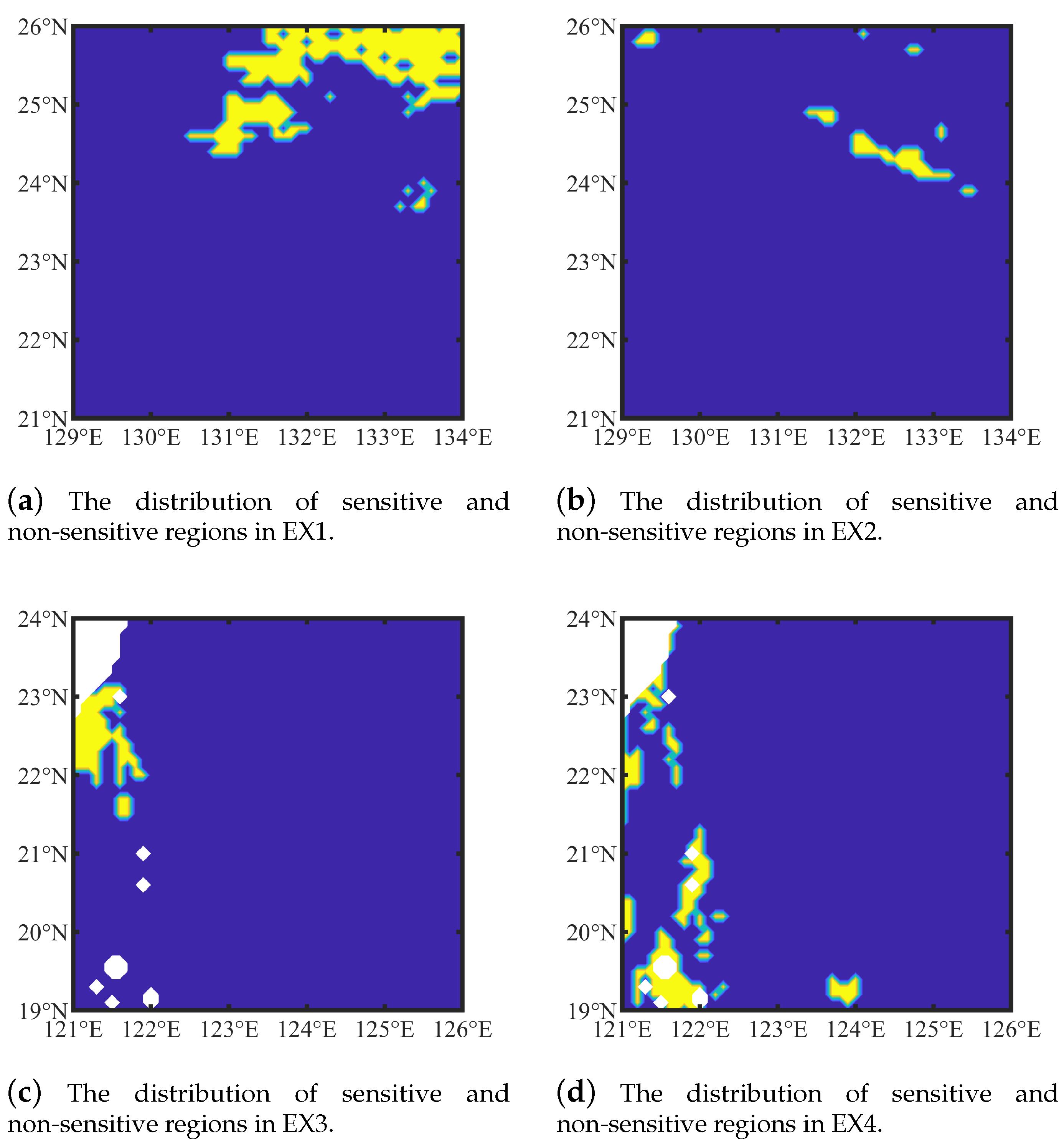
The second set of experiments is as follows: observations are assimilated once in each model integration. However, three problems remain to be solved before the experiments begin. First, whether the CNOP has an error due to prediction error. Second, whether the CNOP changes over time and environment. Third, how to incorporate model uncertainty information in the identification of sensitive regions. Therefore, we compute the CNOPs at different moments in the sampling process and explore the sensitive region based on this idea in Figure 8.

We weighted the CNOP sequence referring to the predictive uncertainty of the model, which reflects the prediction discrepancy between ensemble members. Then, we average the uncertainty of each grid at the same time (the result is shown in the line graph in Figure 8), which can reflect the prediction errors to a certain extent. When the prediction error is small, observations can only slightly improve or even decrease the accuracy of subsequent predictions. The CNOP at such times needs to be assigned less weight. Since the norms of the CNOPs are different and all we need to determine the sensitive regions is the spatial distribution of the CNOP components, we normalize the CNOP sequence for weight convenience. The weighted results are again normalized. Consistent with Figure 5, the target fields are clustered according to the K-means algorithm, and the sensitive and non-sensitive regions are qualitatively analyzed. The results are shown in Figure 9.

Compared to Figure 5, while the general distribution of the sensitive regions in Figure 9 does not change, the details do. In the case of EX1, the sensitive region is greatly expanded. In contrast to the two separated sensitive regions for assimilating multiple observations at once, they are roughly connected for multiple assimilation of multiple observations. In addition, the connected part has a larger component, as can be seen from the normalized target field to the far right of Figure 8. The sensitive region in EX2 is shifted to the left, in EX3 it is concentrated to the right of the land in the upper left corner of the map, and in EX4, the middle and lower parts of the map are also divided into sensitive regions for assimilation of multiple observations.

As in the first set of experiments, OSSE is used to test whether this approach is effective. The sensitive regions identified in the set of experiments are used as the control group; each time the model is integrated, the observations at five locations are assimilated. This procedure is performed several times to avoid experimental errors due to the selection of observation points. The results of OSSE are shown in Figure 10.

It is clear that the prediction quality of the experimental group is better than that of the control group in all four experiments. The mean RMSEs of the control group are 0.12, 0.18, 0.23, and 0.25 in the four experiments. Compared with the control group, the experimental group decreases by 22.83%, 51.89%, 56.75% and 41.60%, respectively, in EX1, EX2, EX3 and EX4. In EX2 and EX4, the RMSE of the experimental group fluctuates considerably. Because after assimilating the observations in the sensitive region, the mean prediction error of the four experimental groups remains substantially below 0.15 K. When the observational error is about 0.1 K, the experiment is more accidental.

4. Design of AUV Sampling Scheme Based on CNOP Spatial Distribution

After studying the ways in which the CNOP sequence can be used for observing missions, we then use the sequence to design an observation scheme for an AUV based on the sampling properties of the autonomous mobile platform. Swarm intelligent optimization algorithms evaluate paths by cost or objective function. The cost function evaluates the cost of the sampling scheme (such as path length, energy consumption), and a smaller cost indicates a better path. The objective function corresponds to the estimated sample value at the critical location of the sampled path, with a larger objective value indicating a better path. Both objective and cost functions are used to evaluate the observation schemes, which are qualitatively similar. When designing the sampling scheme, we can make the cost correspond to the sampling objective by computing the inverse. As for constraints, they can be transformed into costs to form a global cost function, or added to the objective function. The sampling objective function and constraints used in this paper are as follows:

$$\begin{array}{cc}{p}^{*}=\underset{p\in P}{argmax}F(p,O,A,T)& \begin{array}{c}{\wp }_m\notin O\\ L_{min}\le ∥{\wp }_m-{\wp }_{m-1}∥\le L_{max}\\ \begin{array}{cc}{L}_{min}\le ∥{\wp }_m-{\wp }_n∥& m\ne n\end{array}\end{array}\end{array},$$

(7)

where $p=\left\{{\wp }_1,{\wp }_2,\dots ,{\wp }_{\lambda }\right\}$ represent a solution and $p^{*}$ denotes the optimal solution in this problem. P represents a higher dimensional solution space. O is for environmental terrain constraints, or unnavigable areas. A is the attribute constraint of the platform, that is, the sailing distance in a period of time should be neither too large (beyond the navigation capability of the vehicle) nor too small (resulting in repeated observation). T represents task constraint, that is, to avoid repeated observations, a certain distance should be maintained between key sampling locations. F denotes the evaluation index composed of objective function and constraints. $L_{min}$ and $L_{max}$, respectively, represent the minimum and maximum sailing distances of the vehicle in unit time. And m stands for critical position in the voyage, where the course is adjusted.

We design a sampling scheme for an AUV using an improved particle swarm optimization (PSO) algorithm as in Zhao et al., 2023 [20]. This algorithm is optimized for the global adaptive path planning problem by adding a shrinkage operator. The PSO takes the entire observation scheme as a solution and completes the search in a high-dimensional space, so it has a global view in space. In contrast to greedy schemes or other temporal sampling schemes, which progressively select actions sequentially in time until the end of the path is reached, the observation scheme optimized by PSO is less likely to become trapped in a locally optimal solution. Based on Equation (7) and the PSO algorithm, the target fields for sampling and the designed sampling scheme are shown in Figure 11.

The sampling scheme designed in the four experiments successfully passes through the sensitive region. However, this static sampling scheme design approach is not consistent with the actual situation. An obvious difference is that the evaluation does not change when starting and ending positions are swapped. To solve this problem, Zhao et al., 2022 proposed a dynamic objective field design method for a mobile observation platform based on the $\gamma$ discount function [35]. It makes the target field dynamic and more in line with the real situation. However, selection of the optimal $\gamma$ value in the dynamic process is still a problem worth studying.

We use reinforcement learning to optimize the $\gamma$ values of the dynamic target field at different times, thus updating the sampling scheme of the mobile platform. The dynamic target field constructed from prior information at subsequent moments allows the design of sampling schemes with a global view in time. The dynamic adaptive observation scheme design method for AUV with spatio-temporal global vision is divided into two modules and the relationship between them is shown in Figure 12.

On the left is the prior information processing module based on reinforcement learning. In designing sampling schemes using prior information, historical and current information are no longer required. Since the observation scheme is continuously updated in the subsequent process, the values of future information at different times in the present moment are not equal. To match the actual process, the future information closest to the current moment is given a larger weight in the construction of the target field, and subsequent information is discounted when it is utilized. The further away from the current moment, the greater the discount. Reinforcement learning adaptively adapts the discount values to facilitate the decision of the optimal sampling scheme. A swarm intelligent optimization algorithm is used to generate the sampling scheme, whose objective function consists of two parts: one is the objective itself, which is the sample value estimation matrix of the spatial distribution. Others are constraints, including terrain constraints to prevent the sampling paths of AUVs with obstacles from intersecting, which increases the risk of navigation; platform attribute constraints prevent the design of sampling schemes that go beyond the navigation capabilities of mobile platforms; the observation objective constraint prevents AUV from repeatedly sampling regions with high estimated sample values. The objective function provides an evaluation criterion for the quality of the sampling scheme. The population evolution strategy of the swarm intelligent optimization algorithm is applied to the population evolution to provide new ensembles of candidate sampling schemes for iteration. Details of the problem model and observation scheme design are presented in Zhao et al., 2022 [35]. For the swarm intelligent optimization algorithm part, we use the improved PSO algorithm mentioned above. For the reinforcement learning part, we use the Q-learning algorithm to adjust discount from different moments. The formula is as follows:

$$NewQ(s,a)=Q(s,a)+\alpha \left[R(s,a)+{\gamma }_{l}max{Q}^{\prime }\left(s^{\prime },a^{\prime }\right)-Q(s,a)\right],$$

(8)

where Q is a state action function that is iterated during learning. $Q(s,a)$ represents the Q value corresponding to action a at state s. In this paper, the state refers to the position information of the vehicle corresponding to different sampling moments, and the action refers to the $\gamma$ value selected for the subsequent prior information when making the next observation scheme decision. $R(s,a)$ represents a real-time reward for the current action; here, it corresponds to an estimate of the value of the sample collected at the next time. $\alpha$ and ${\gamma }_l$ are the learning and discount rates, which belong to the parameters of the algorithm. There is a difference between ${\gamma }_l$ here and $\gamma$ optimized: the former is an internal parameter of the algorithm, and the latter is the discount given when applying the CNOP sequence. $Q^{\prime }\left(s^{\prime },a^{\prime }\right)$ represents the Q value corresponding to the action $a^{\prime }$ in the next phase (state $s^{\prime }$). The setup of the basic parameters in constraints, the improved PSO and the Q-learning is shown in

Table 2. The setup of the basic parameters in constraints, the improved PSO and the Q-learning.

The Setup of the Basic Parameters
Parameters in constraints	$L_{min}$	$L_{max}$	The interval between two adjustments
Value	11 km	27 km	6 h
Parameters in the improved PSO	Population size	Maximum iterations	Number of populations
Value	15	1000	20
Parameters in the Q-learning	$\alpha$	${\gamma }_l$	Maximum iterations
Value	0.1	0.9	200

.

Other parameters of the improved PSO algorithm are adjusted in an adaptive way with the number of iterations. The specific setting method is described in Zhao et al., 2023 [20]. The sampling scheme obtained based on this method is shown in Figure 13. To better reflect the observation characteristics of the mobile platform, we use different subgraphs representing different moments to reflect the dynamic sampling process. The sampling scheme based on the static target field is used as the control group. It can be seen intuitively from Figure 13 that at the sampling time corresponding to the subgraph (d, e, i), compared with the sampling scheme designed based on the static target field, the sampling scheme designed based on the dynamic target field falls more in the dark gray sensitive region.

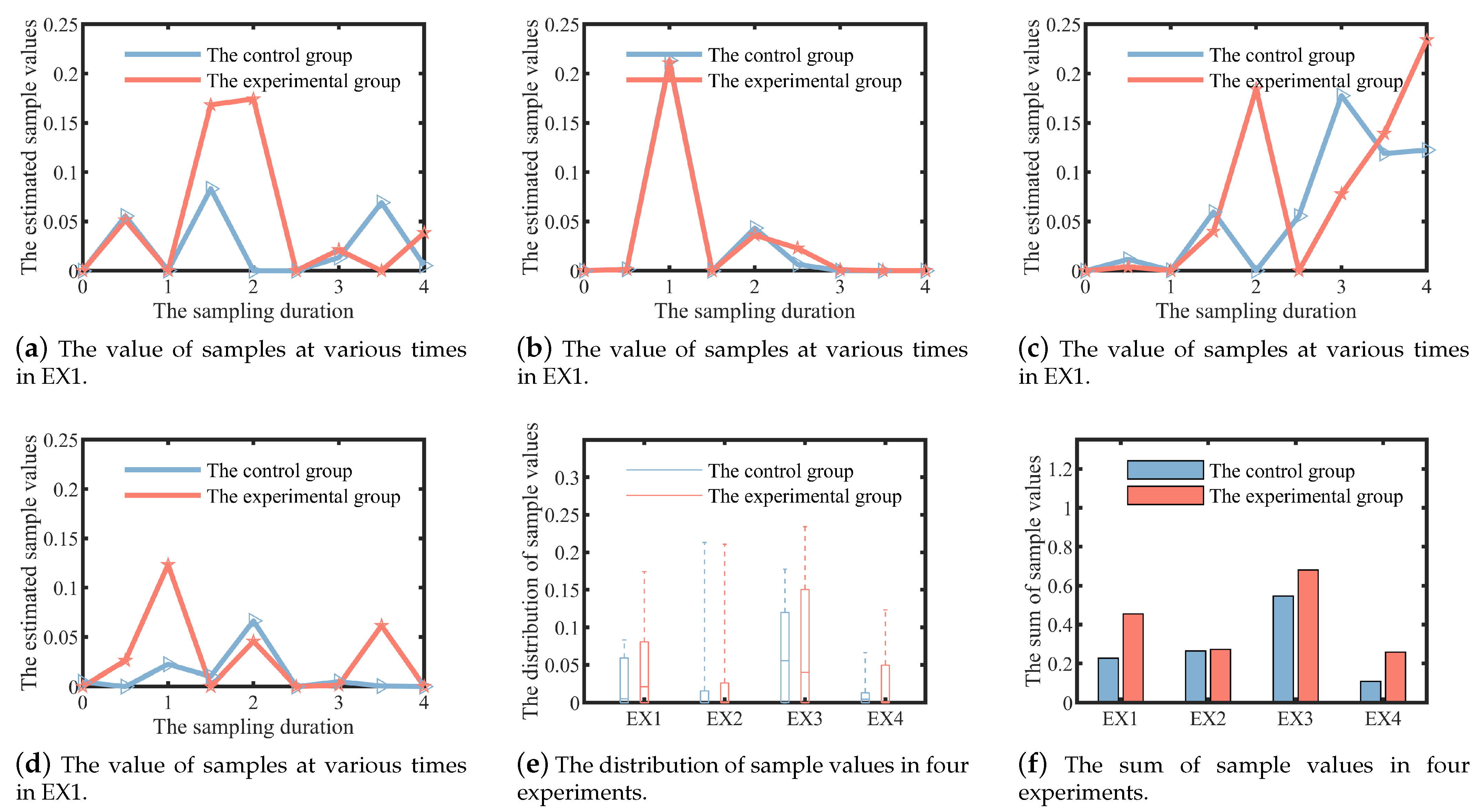
We further quantitatively compare the estimated value of the samples collected in different times between the two schemes. The results of the four experiments are shown as line plots in Figure 14. For analytical convenience, the overall distribution and the mean of the sample values are also plotted in Figure 14 as box and bar plots.

The optimal observation path we seek implies a global optimum. That is to say, at some point, the experimental group does not sample as well as the control group (e.g., Day 3.5 of EX1 and Day 2 of EX2). But the general trend is that the experimental group outperforms the control group. The most obvious comparison is EX1, where the best sample value is less than 0.1 for the control group and greater than 0.15 for the experimental group. As can be seen from the box diagram in Figure 14e, in EX1, the experimental group is significantly higher than the control group in terms of the maximum, upper quartiles or median of the estimated sample value. This overall optimal is more easily reflected by the sum value of the sample shown in Figure 14f. The sum values of the estimated samples obtained in the four experiments are 0.23, 0.26, 0.55, and 0.11, respectively, in the control group. The experimental group is better than the control group in four experiments (The improvement effects are 99.94%, 2.87%, 24.42% and 136.37%, respectively), which shows that the sampling scheme design method based on dynamic target field is effective.

In order to test the actual sampling effect of the sampling scheme, OSSE is carried out. The specific setting of the experiment is shown in Figure 15. Unlike the OSSE mentioned above, this experiment simulates the dynamic sampling process of an AUV. Thus, during the model integration, for each assimilated observation, the corresponding spatial location is different. The time window for assimilation is chosen to be 6 h. The advantage of the mobile sampling platform is its flexibility and mobility, which can change the observation position according to the environment. When the number of mobile platforms is small and the observation range is large, the number of samples obtained by this method is small compared with that of a large number of fixed platforms. In order to simulate this feature, we assume that six hours of sampling provides information on a location. The results are shown in Figure 16.

After combining the observation with the forecast through the data assimilation to form the optimal estimation of the ocean state and applying it to the forecast of the next stage, we can see that the predicted RMSE values at the next moment based on the sampling scheme designed by the static target field are 0.37 K, 0.25 K, 0.28 K, 0.29 K in the four experiments, respectively. The predictions of the experimental group are improved by 3.94%, 1.68%, 5.12% and 0.68%, respectively, compared with the control group. Compared with Figure 9, sampling based on mobile platform does not significantly improve the forecast (the forecast error after improvement is still above 0.25 K), because fewer observations are collected in this experiment to simulate the observation characteristics of the mobile platform. It is important to note that this error is the error in our simulation environment, which is relatively small compared to the real situation. Moreover, in Figure 13 and Figure 14, there are obvious differences between control group and experimental group, but the rate of RMSE in the four experiments is basically less than 6%. This is because the estimated sampling values in this paper do not strictly correspond to the actual sampling values, and errors in the simulation experiments can also affect the sampling results. And, despite the differences between the observation schemes of the control and experimental groups, the overall improvement is limited by the fact that only two observations are assimilated at a time in the simulated experiment. In the future, we will validate the proposed methodology for designing observational schemes by combing with CNOP, based on a more refined model, while tracking more practical variables such as underwater temperature and vertical gradient through a 3D environment. These results show that the sampling scheme based on dynamic design method is more effective in improving the prediction accuracy of the numerical model.

5. Summary and Discussion

To integrate the two problems of where to observe and how to observe, we combine targeted observation with sampling scheme design for a mobile platform. First, we compute the fastest growing perturbations and divide the sensitive region by clustering based on the spatial distribution. With OSSE, we verify that sampling in the sensitive region is more efficient than the non-sensitive region to improve prediction accuracy. Then, in combination with the model uncertainty estimation, we design a sampling scheme based on the observational characteristics of the mobile observing platform. In this paper, we aim to apply the theoretically sensitive region to the design of sampling schemes for mobile platforms to maximize observing efficiency.

First, we apply the CNOP method to nested ICCM via an intelligent approach. To reduce the randomness of the experiments, we perform four experiments at different times and in different regions. The sensitive regions are divided by clustering, and the OSSE is performed by selecting the same number of observation sites in different regions. The results show that the improvement effect of forecast is more obvious by assimilating samples collected in sensitive region than in the non-sensitive regions. However, the improvement (not more than 0.05 K) is limited due to the short sampling duration. Based on this, we perform OSSE on continuous sampling. The CNOPs at different times are weighted by prediction uncertainty. Again, the sensitive region is divided by clustering. OSSE is completed by taking an equal number of samples from the newly identified sensitive region and the original sensitive region. The results show that sampling in the newly identified sensitive regions is more efficient. In the most significant group of the four experiments, the predicted RMSE is reduced by 56.75%, and other experiments also showed reductions of more than 20%. Then, after verifying that observations in the sensitive region are more effective for improving the prediction, combined with the character of the mobile platform, we apply the method for estimating the sensitive region in the design of a sampling scheme. We combine a modified Q-learning and PSO algorithm to propose a hybrid approach, which is used to integrate the most sensitive initial perturbations at different times and generate an observation scheme. Finally, we analyze the sampling scheme designed by this method from two perspectives of objective function value and OSSE. The scheme designed in the static target field is used as a control group. The static target field is formed by weighting the optimal perturbations at different times, regardless of dynamical changes. Both the optimization and OSSE results show that the sampling scheme designed by dynamic method is more effective. In the most obvious group of the four experiments, the optimization results of the sampling scheme are doubled. In the OSSE results, the predicted RMSE of the experimental group also decrease by about 0.3 K in all four experiments compared to the control group, with the most pronounced decrease reaching more than 5%. Considering different sampling durations and observing characteristics, these results provide theoretical support for designing observing schemes in combination with CNOP.

While the combination of CNOP and the observation scheme improves the prediction of nested ICCM, serious challenges remain for applications. First, in the present study, we only use a two-dimensional structure plane model, which is limited in reflecting the coupled circulation processes of the atmosphere and ocean. In the future, we will combine a more realistic model (for instance, HYCOM [22] or NEMO [23]) to extend this method to a three-dimensional scene. Second, we design the observing scheme by combining the observed features of each platform in isolation, which is not consistent with reality. A way to combine the different observing platforms for collaborative observations remains a question worth investigating. Third, in designing the sampling scheme, we simply combine a basic reinforcement learning and swarm intelligence algorithm, which will be continuously improved to achieve better optimization results.