Influence of Blade Flexibility on the Dynamic Behaviors of Monopile-Supported Offshore Wind Turbines

Abstract

At present, monopile-supported offshore wind turbines (MOWTs) are widely used in offshore wind farms. The influence of blade flexibility on the dynamic behaviors of MOWTs excited by waves and earthquakes was investigated in this study. Numerical analysis models were established for 5 MW and 10 MW MOWTs, incorporating flexible and rigid blade configurations. The modes and natural frequencies of the full system were compared between these two numerical models, and their dynamic responses were evaluated under wave-only and earthquake-only excitations. It was revealed that the influence of blade flexibility on the first- and second-order modes of the system can be neglected. The dynamic response of these MOWTs under wave excitation can be predicted by the rigid blade model, where the maximum relative difference is less than 5%. However, higher-order modes of the system are significantly affected by the blade flexibility. Under high-frequency excitations, these higher-order modes of the system are remarkably stimulated. Additionally, a large relative difference, exceeding 50%, is detected when the rigid blade model is used to predict the seismic response of the two MOWTs. Consequently, the blade flexibility should be adequately modeled when predicting the dynamic response of OWTs.

1. Introduction

Offshore wind energy offers greater abundance and stability than onshore, and its exploration has less impact on the environment [1]. Consequently, offshore wind energy is a promising option. According to the Global Wind Energy Council [2], the global installed capacity of offshore wind power reached 8.8 GW in 2022. To reduce the levelized cost of wind power, more and more large-scale wind turbines have been installed [3]. However, these wind turbines are more susceptible to dynamic excitations due to the large mass of the rotor–nacelle assembly (RNA) and the flexibility of the support structure. Therefore, accurately predicting the dynamic behavior of offshore wind turbines (OWTs) is crucial to ensure their structural integrity and economic viability.

Currently, the majority of commercial offshore wind energy plants are located in nearshore areas and utilize bottom-fixed support structures. Bottom-fixed OWTs are subjected to long-term dynamic forces from the marine environment [4]. Additionally, in regions with significant seismic hazards, bottom-fixed OWTs face damage risks induced by strong ground motion [5]. The bottom-fixed OWTs consist of a foundation, substructures, tower, nacelle, and rotor [6]. Therefore, the dynamic analysis of OWTs requires appropriate modeling of structural characteristics, whether through theoretical analysis [7] or experiment [8].

The rotor, which consists of blades and a hub, is the crucial component of OWTs. It plays a vital role in converting wind energy into electricity by rotating with the low-speed shaft of the drivetrain system [9]. Currently, there are two types of modeling methods for the dynamic analysis of OWTs in terms of blades. The first type involves establishing a blade model with distributed mass and stiffness properties, which is referred to as the flexible blade model in this study. The beam element is usually used to model the mass, stiffness, and damping distribution of blades [10,11]. To decouple the aero-elastic effect, aerodynamic damping was introduced into the numerical model through a viscous damper [12] or modal damping [13]. This improvement allows for the dynamic response of OWTs under wind and other load excitations to be computed in general software. For example, the commercial finite element software ABAQUS was used to establish a numerical model for MOWTs excited by wind, waves, and earthquakes [14,15]. Along this line, researchers have developed a detailed blade model to analyze the dynamic behavior of the DTU 10 MW wind turbine under seismic action [16,17], where the skin and spar of blades are modeled by the shell element. However, the complex modeling or manufacturing methods, as well as the limited blade structural information, constrain the application of flexible blade models in numerical simulations and experimental research.

The second type of method treats the rotor as a rigid body and only considers its inertial effects. Although there may be some differences in determining the total mass and inertia moment of the RNA, the commonality among these methods is that blade stiffness is not taken into account. Consequently, it is referred to as the rigid blade model in the current study. Bazeos et al. [18] established a finite element model for a 450 kW wind turbine. In this research, the RNA was modeled by a concentrated mass and its aerodynamic loads were simplified as a quasi-static concentrated force. Based on this model, seismic responses of wind turbines at the operational state were analyzed [19], and the dominant role of earthquake load at high-seismic-hazard regions was emphasized [20]. However, it is difficult to consider the aero-elastic effect by using this model, which restricts the applicability of this simplified model.

As wind turbines grow larger, the flexibility of the blades increases, necessitating the consideration of the aero-elastic effect when computing the aerodynamic loads on the rotor [21]. To meet this requirement, researchers computed the hub-height aerodynamic loads using aero-elastic software and then established a finite element model using the hydro-geotech code USFOS [22,23], where the RNA was also simplified as a concentrated mass. This model has been utilized to investigate the dynamic behavior of OWTs under various loads, such as extreme wind and wave conditions [24], earthquakes [25,26], normal ocean states [27], etc. In summary, rigid blade models have been proposed and improved by researchers. Additionally, these models have been widely applied in the dynamics of OWTs, including theoretical analysis [28], experimental research [29], and numerical simulations [30]. However, the applicability of these models has not been reported.

On the whole, the influence of blade flexibility on the dynamic response of OWTs stems from the impact of blade oscillation velocity on aerodynamic loads and the effect of blade stiffness on the system’s dynamic characteristics. The former has already become a consensus in the wind power industry, and researchers have demonstrated the impact of blade flexibility on aerodynamic loadings through numerical analysis [31] and wind tunnel experiments [32]. As for the influence of blade stiffness on dynamic characteristics and the dynamic response of OWTs, the existing research is quite limited. Arany et al. [33] proposed a closed solution for the first-mode natural frequency of MOWTs by modeling the RNA as a concentrated mass. This solution was validated by comparison with experimental results. To some extent, their work suggests that the rigid blade model may be used to predict the natural frequency of MOWTs. The rigid blade model has been extensively used to analyze the dynamic response of different loadings. However, to the best of the author’s knowledge, no researchers have investigated whether it is applicable for predicting higher-order modes and dynamic responses of multi-megawatt OWTs.

To address the research gap in this field, the present study explored the influence of blade flexibility on the dynamic behaviors of MOWTs. The outline of this study is as follows: firstly, the characteristics of 5 MW and 10 MW MOWTs, the properties of the blade, load cases, the numerical model, and methodology are summarized; secondly, the modes and natural frequencies of 5 MW and 10 MW MOWTs are analyzed by using flexible and rigid blade models, respectively; thirdly, the dynamic response of 5 MW and 10 MW MOWTs excited by waves and earthquakes only are analyzed and compared; finally, some conclusions are summarized.

2. Model, Load Cases, and Methodology

2.1. Characteristics of MOWTs

This study aimed to explore the influence of blade flexibility on the dynamic behaviors of multi-megawatt OWTs. Specifically, two MOWTs were analyzed, one utilizing the NREL 5 MW reference wind turbine [34] and the other incorporating an update on the DTU 10 MW wind turbine [35]. Both of them are upwind horizontal axis wind turbines with three blades. Their control systems adopt variable speed and blade pitch technology. These reference wind turbines have been extensively utilized in previous studies [36,37]. The main characteristics of the two MOWTs are summarized in

Table 1. Properties of the 5 MW and 10 MW monopile-supported OWTs.

Part	Property	NREL 5 MW	DTU 10 MW
Blade	Rotor diameter	126 m	178.3 m
	Hub height	90 m	119 m
	Cut-in, rated, and cut-out wind speed	3 m/s, 11.4 m/s, and 25 m/s	4 m/s, 11.4 m/s, and 25 m/s
	Cut-in and rated rotor speed	6.9 rpm and 12.1 rpm	6.0 rpm and 12.1 rpm
	Length	61.5 m	86.35 m
	Overall mass	53,220 kg	122,442 kg
	Structural damping ratio	0.5%	0.5%
Hub and nacelle	Hub diameter	3 m	5.6 m
	Hub mass	56,780 kg	105,520 kg
	Nacelle mass	240,000 kg	446,036 kg
Tower	Bottom and top outer diameter	6 m and 3.87 m	7.8 m and 5.3 m
	Bottom and top wall thickness	0.027 m and 0.019 m	0.05 m and 0.03 m
	Overall mass	347,460 kg	673,998 kg
	Structural damping ratio	1%	1%
Monopile	Total length	66 m	69 m
	Outer diameter	6 m	7.8 m
	Wall thickness	0.060 m	0.085 m

. Detailed information on the two wind turbines can be found in the literature [34,35].

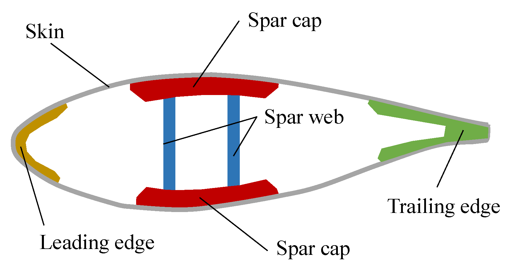
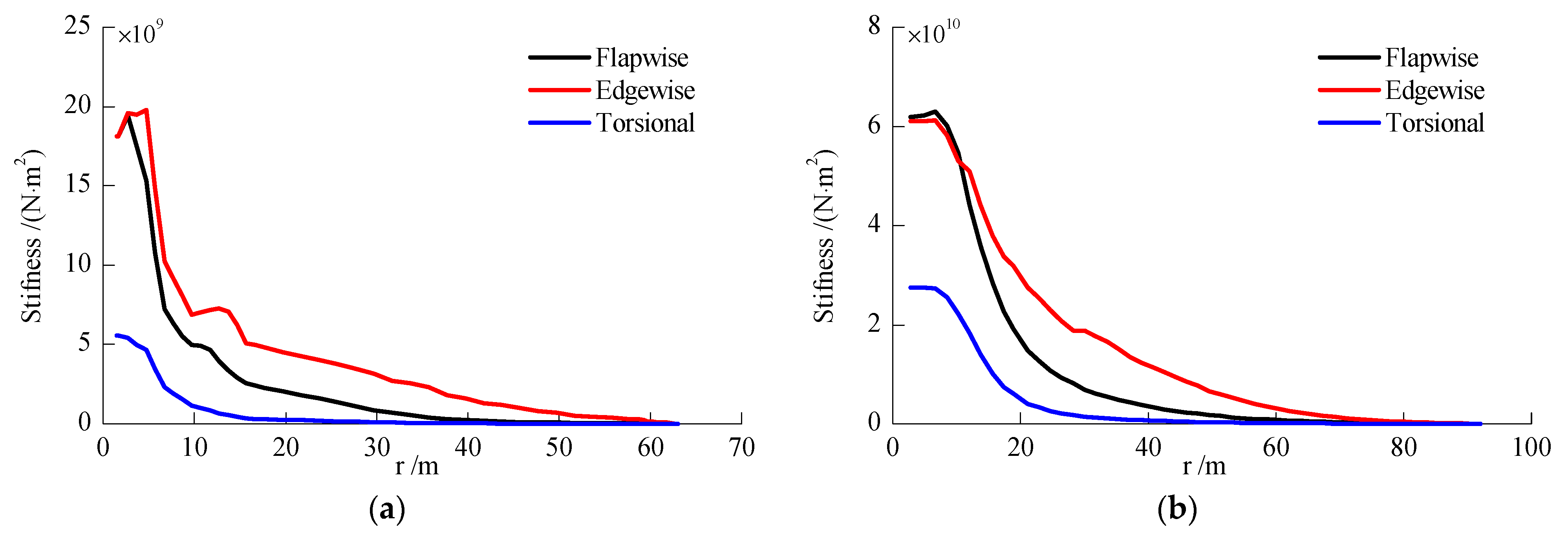
2.2. Properties of the Blade

Wind turbine blades are slender members and exhibit characteristics of cantilevered beams [9]. Functionally, the structure of a blade can be divided into two components: the skin and the spar [17]. The skin forms the outer geometry of the blade and endures a portion of the aerodynamic and mechanical loads. The spar plays a crucial role as the load-bearing element, typically comprising a spar cap and a spar web, as shown in Figure 1. The spar cap supports the bending loads generated by the aerodynamic and mechanical forces. The spar web resides within the hollow section of the spar cap, providing reinforcement, enhancing stiffness, and preventing structural buckling [38]. The spar cap is usually constructed using unidirectional fabrics, while the spar web adopts a sandwich structure.

To meet the structural requirements, a variable cross-section is employed in the blade design. Taking the 10 MW turbine as an example, the FFA-W series airfoils are utilized [35]. The airfoils along the blade span include FFA-W3-241, FFA-W3-301, FFA-W3-360, FFA-W3-480, and FFA-W3-600, with relative thicknesses of 24.1%, 30.1%, 36%, 48%, and 60%, respectively. The variations in blade mass and cross-sectional stiffness as a function of the radial distance “r” are presented in Figure 2 and Figure 3 for the 5 MW and 10 MW wind turbines, respectively. This study aimed to investigate the influence of blade flexibility on the dynamic behaviors of the support structure. Consequently, the blade was modeled as a beam with varying cross-sections.

2.3. Load Cases

To assess the impact of blade flexibility, both low-frequency and high-frequency excitations were applied to these two OWTs. For bottom-fixed OWTs, although both wind and waves are low-frequency excitations, wind loadings on blades are significantly affected by the aero-elastic effect and control system. Under the wind excitation, the blade flexibility influences the dynamic responses of OWTs through the combined effect of wind loads and system dynamic characteristics. Based on the purpose of this work, the wind turbines were assumed to be in the parked condition, neglecting the influence of wind. Consequently, the low-frequency and high-frequency excitations were generated by waves and earthquakes, respectively.

In this study, an irregular wave model was used to represent the real sea state. A power spectrum should be selected to describe the amplitude of the wave component. The JONSWAP spectrum is frequently utilized in the dynamic analysis of MOWTs. It is also proposed by guidelines of the offshore wind energy community [39] and the report of 10 MW MOWTs [35]. Consequently, the JONSWAP spectrum used in this study is as follows:

$$S\left(f\right)=\frac{\alpha {\mathrm{g}}^2}{{\left(2\mathsf{\pi }\right)}^4}{f}^{-5}\exp \left(-\frac{5}{4}{\left(\frac{f}{f_{\mathrm{p}}}\right)}^{-4}\right){\gamma }^{\exp \left(-0.5{\left(\frac{f-f_{\mathrm{p}}}{\sigma ·f_{\mathrm{p}}}\right)}^2\right)}$$

(1)

where $f$ represents the wave frequency, $f_{\mathrm{p}}$ denotes the spectral peak frequency, g is the acceleration of gravity, $\alpha$ represents the generalized Phillips’ constant, $\mathsf{\sigma }$ is the spectral width parameter, and $\gamma$ denotes the peak-enhancement factor. These parameters are either constants or can be determined based on their relationship with the significant wave height H_s and peak period T_p.

In designing the support structures for these two OWTs, the metocean data of the Ijmuiden Shallow Water Site were used. This site is located in the Dutch North Sea and the water depth is 21.4 m MSL. The coordinates of this site are 52°33′00″ east and 4°03′30″ north. The metocean data are based on 3 h average values for a period of 22 years (January 1979–December 2000). The dynamic analysis of these OWTs employed the wave parameters of this site. The most significant wave height and peak periods are summarized in

Table 2. Parameters of the wave spectrum.

Load Cases	Significant Wave Height Hs (m)	Peak Period Tp (s)	Description
1	1.67	5.89	Hub mean wind speed 12 m/s
2	3.72	8.11	Hub mean wind speed 26 m/s
3	4.75	9.09	Hub mean wind speed 32 m/s
4	6.06	9.71	Return period 1 year

. More details about the metocean condition of this site can be found in the report by Fischer et al. [40].

The input earthquakes were selected considering the recommendation of the Applied Technology Council (ATC) [41]. These records include far-field, near-field, and pulse-like seismic motions, as specified in

Table 3. Earthquake ground motions.

No.	Earthquake, Year	Station/Component	No.	Earthquake, Year	Station/Component
1	Kocaeli, 1999	Arcelik/000	28	Duzce, 1999	Duzce/180-pulse
2	Duzce, 1999	Bolu/000	29	Imperial Valley-06, 1979	El Centro Array-6/230
3	Loma Prieta, 1989	Capitola/000	30	Imperial Valley-06, 1979	El Centro Array-7/140
4	Chi-Chi, 1999	CHY101/E	31	Erzican, 1992	Erzincan/s
5	Imperial Valley, 1979	Delta/262	32	Kocaeli, 1999	Izmit/090
6	Kocaeli, 1999	Duzce/180	33	Landers, 1992	Lucerne/260
7	Imperial Valley, 1979	El Centro Array-11/140	34	Cape Mendocino, 1992	Petrolia/090
8	Loma Prieta, 1989	Gilroy Array-3/090	35	Superstition Hills-02, 1987	Parachute Test Site/225
9	Hector Mine, 1999	Hector/090	36	Northridge-01, 1994	Rinaldi Receiving Sta/228
10	Superstition Hills, 1987	El Centro Imp. Co./090	37	Loma Prieta, 1989	Saratoga-Aloha/090
11	Northridge, 1994	Canyon Country-WLC/000	38	Irpinia, Italy-01, 1980	Sturno/270
12	Northridge, 1994	Beverly Hills-Mulhol/009	39	Northridge-01, 1994	Sylmar-Olive View/360
13	Kobe, 1995	Nishi-Akashi/000	40	Chi-Chi, 1999	TCU065/E
14	San Fernando, 1971	LA-Hollywood Stor./090	41	Chi-Chi, 1999	TCU102/E
15	Superstition Hills, 1987	Poe Road (temp)/360	42	Northridge-01, 1994	LA-Sepulveda VA/7360
16	Cape Mendocino, 1992	Rio Dell Overpass/270	43	Imperial Valley-06, 1979	Bonds Corner/140
17	Kobe, 1995	Shin-Osaka/000	44	Loma Prieta, 1989	BRAN/000
18	Friuli, 1976	Tolmezzo/000	45	Imperial Valley-06, 1979	Chihuahua/282
19	Landers, 1992	Yermo Fire Station/270	46	Loma Prieta, 1989	Corralitos/000
20	Manjil, 1990	Abbar/T	47	Gazli, 1976	Karakyr/gaz0
21	Darfield, 2010	Christchurch Cathedral College/26w	48	Nahanni, 1985	Site 2/240
22	ChiChi, 1999	Chy104/chy104-n-004	49	Nahanni, 1985	Site 1/010
23	Mexico, 2010	Calexico Fire Station/ cxo090	50	Northridge-01, 1994	Northridge-Saticoy/090
24	Mexico, 2010	Cerro Prieto Geothermal/ geo000	51	Chi-Chi, 1999	TCU067/E
25	Darfield, 2010	Christchurch Hospital/ hcs89w	52	Chi-Chi, 1999	TCU084/E
26	Chi-Chi, 1999	TCU070/tcu070-n	53	Kocaeli, 1999	Yarimca/330
27	Chi-Chi, 1999	TCU109/tcu109-n

. Both the wave and seismic motions are parallel to the horizontal projection of the normal vector of the rotor plane. The interaction between water and the oscillated monopile is considered by the updated added mass method proposed by Wang et al. [30].

2.4. Numerical Model

To examine the influence of blade flexibility, the natural frequencies and mode shapes of the system were compared using both flexible and rigid blade models. Finite element models were created for these two MOWTs using the ADINA software [42], with three-dimensional beam elements utilized to simulate the blades and support structure. The length of the blade and monopile element was set to 1 m, and the length of the tower element was set to 2 m. The blades and support structures are both made of linear elastic materials whose parameters are summarized in

Table 4. Material properties of wind turbines.

ID	Mass Density ρ (kg/m3)	Young’s Modulus E /GPa	Poisson’s Ratio μ	Shear Modulus G /GPa	Description
1	1500	20	0.2	8.33	Flexible blade
2	7800	200	0.3	76.92	Support structure
3	1500	200,000	0.2	83,300	Rigid blade

. Since the ADINA software does not have a rigid material, the Young’s modulus of the blade was increased by 10,000 times in the rigid blade model, which corresponds to material 3 in Table 4. This approach allows for neglecting the deformation of the blade and treating it as a rigid body.

The cross-sections of the tower and monopile for these two OWTs were modeled by the ‘pipe’ form of ADINA, and the outer and wall thickness was determined based on Table 1. Considering that the blades are composed of multiple materials and have a complex structure, their sections were modeled using the ‘general’ form in the ADINA software. The area A, moment of inertia I, and polar moment of inertia I_p of the cross-section for blades were determined via the following equations:

$$A=\frac{\overline{m}}{\rho }$$

(2)

$$I=\frac{EI}{E}$$

(3)

$$I_{\mathrm{p}}=\frac{G{I}_{\mathrm{p}}}{G}$$

(4)

where $\overline{m}$, $EI$, and $G{I}_{\mathrm{p}}$ are the distributed mass per length, bending stiffness, and torsional stiffness, respectively; $\rho$, $E$, and $G$ are the material mass density, Young’s modulus, and Poisson’s ratio, respectively. These distributed properties of the cross-section are summarized in the corresponding report [34,35]. The hub and generator are represented as concentrated masses, while the nacelle, for which stiffness data are unavailable, is considered a rigid body.

The dynamic responses of the two MOWTs under investigation were simulated using the GL-Bladed software [43], with beam elements employed to represent the blades and tower. For the blade, the cross-section properties, i.e., distributed mass, stiffness, and airfoil, should be directly inputted by users. The rigid blade model was implemented by disabling the ‘flexibility’ option of the blade in the GL-bladed software. For the tower and monopile, this software calculates the distributed mass and stiffness data based on their geometry dimension and material properties. These models adopt the same mesh size as those established in ADINA.

These numerical models incorporate the beam on the nonlinear Winkler foundation (BNWF) model to simulate the soil–structure interaction (SSI) between the soil and monopile foundation. The horizontal reaction curve of the foundation employs an improved model that takes into account the size effect of large-diameter piles, as shown in the following [44]:

$$P={\mathrm{AP}}_{\mathrm{u}}\tan \mathrm{h}\left[\frac{k_0{\mathrm{z}}_0{\left(\frac{D}{{\mathrm{D}}_0}\right)}^m{\left(\frac{z}{{\mathrm{z}}_0}\right)}^n}{{\mathrm{AP}}_{\mathrm{u}}}y\right]$$

(5)

where A is a factor accounting for the cyclic or static loading conditions, evaluated by A = 0.9 for cyclic loading; P_u is the ultimate lateral resistance at depth z; k₀ is the initial stiffness of the foundation; z₀ = 2.5 m is the reference depth; z is the depth below the original seafloor; y is the lateral deflection at depth z; D is the monopile outside diameter; D₀ = 1.0 m is the reference diameter of the monopile; and m = 0.5 and n = 0.6 are dimensionless coefficients.

In fact, the horizontal reaction curve is commonly referred to as the p-y curve. The support structures of both MOWTs are designed for the site depicted in Figure 4, where γ and φ are the effective soil unit weight and soil internal friction angle, respectively. As a result, these parameters were utilized to establish the SSI model for the two OWTs. The BNWF model was implemented by using springs along the pile shaft under the seabed. Given that modal analysis is conducted for linear systems, the initial slope of p-y curves was used as the stiffness of springs for modal analysis in ADINA. In dynamic analysis, these p-y curves are used as the force–displacement relationship of springs for the GL-bladed model.

2.5. Methodology

During modal analysis, in order to ensure the non-singularity of the stiffness matrix, the RNA is rigidly connected to the tower top. Soil springs are placed along the pile shaft. In the standard finite element procedure, the motion equation of the system can be represented as follows:

$$\left[\mathit{M}\right]\left\{\ddot{\mathit{u}}\right\}+\left[\mathit{K}\right]\left\{\mathit{u}\right\}=\left\{0\right\}$$

(6)

where $\left[\mathit{M}\right]$ and $\left[\mathit{K}\right]$ are the mass and stiffness matrices, respectively; $\left\{\mathit{u}\right\}$ and $\left\{\ddot{\mathit{u}}\right\}$ are the displacement and acceleration vectors, respectively. In this equation, the difference between the flexible blade model and the rigid blade model lies only in the stiffness matrix. The Enriched Bathe subspace iteration method [45] was employed to implement the modal analysis for the flexible blade and rigid blade models.

In GL-bladed, the principle of virtual work is utilized to integrate the motion equations of the system, which can be expressed as the following:

$$\left[\mathit{M}\right]\left\{\ddot{\mathit{u}}\right\}+\left[\mathit{C}\right]\left\{\dot{\mathit{u}}\right\}+\left[\mathit{K}\right]\left\{\mathit{u}\right\}=\left\{\mathit{f}\right\}$$

(7)

where $\left[\mathit{C}\right]$ is the damping matrix, $\left\{\dot{\mathit{u}}\right\}$ is the velocity vector, and $\left\{\mathit{f}\right\}$ is the load vector. For structural damping, as recommended in the report, the damping ratio for all modes was assumed to be 0.5%. The foundation damping is generated by radiation and hysteresis effects. The model developed by Makris and Gazetas [46] was used to determine the foundation damping as follows:

$$c_{\mathrm{s}}=6\sqrt{{\rho }_{\mathrm{s}}{G}_{\mathrm{s}}}D{\left(\frac{{\omega }_{1}D}{\sqrt{G_{\mathrm{s}}/{\rho }_{\mathrm{s}}}}\right)}^{-1/4}+2{\beta }_{\mathrm{s}}\frac{k_{\mathrm{s}}}{{\omega }_1}$$

(8)

where c_s is the foundation damping coefficient; ρ_s and G_s are the density and shear modulus of the soil, respectively; ω₁ is the first-order natural angular frequency of the support structure; k_s is the initial stiffness of the p-y curves; and β_s is the hysteresis damping ratio with a value of 5%. The shear modulus of the soil for the site illustrated in Figure 4 was taken from the literature [47]. For the sake of brevity, it is not listed here again. The Morison equation was used to calculate wave loadings, which are applied to the support structures under the sea surface. The input seismic acceleration was converted into inertial forces by GL-bladed and applied to the entire system. Subsequently, these loads are integrated into the load vector in Equation (7). To improve the computational efficiency, the fourth-order Runge–Kutta method with a variable time step was used to solve the motion equations of the system.

For the dynamic analysis implemented in GL-bladed, a modal reduction method was applied to reduce computational burden by considering a reduced number of support structures and blade modes. The full finite element model was used as the benchmark method to explore the modal reduction models required for computational accuracy, considering different mode numbers. Taking the Duzce record (no. 28 of Table 3) as the input earthquake, the 5 MW and 10 MW MOWTs use 8 and 12 modes for the blades, respectively, while their support structures use 20 modes. Their seismic responses are shown in Figure 5 and Figure 6. The modal reduction models exhibited high agreement with the full finite element models. In addition, more studies with other input earthquakes indicate that these modal reduction models achieve a balance between computational accuracy and efficiency, and they are used for implementing dynamic analysis.

3. Results and Discussion

This section utilizes two software packages, namely ADINA and GL-Bladed, to conduct all numerical analyses. These commercial software packages have been certified for their accuracy, as documented in their respective user manuals. Therefore, the validation of numerical modes focuses on assessing the reliability of the modeling process, which is implemented by a comparative analysis with existing studies.

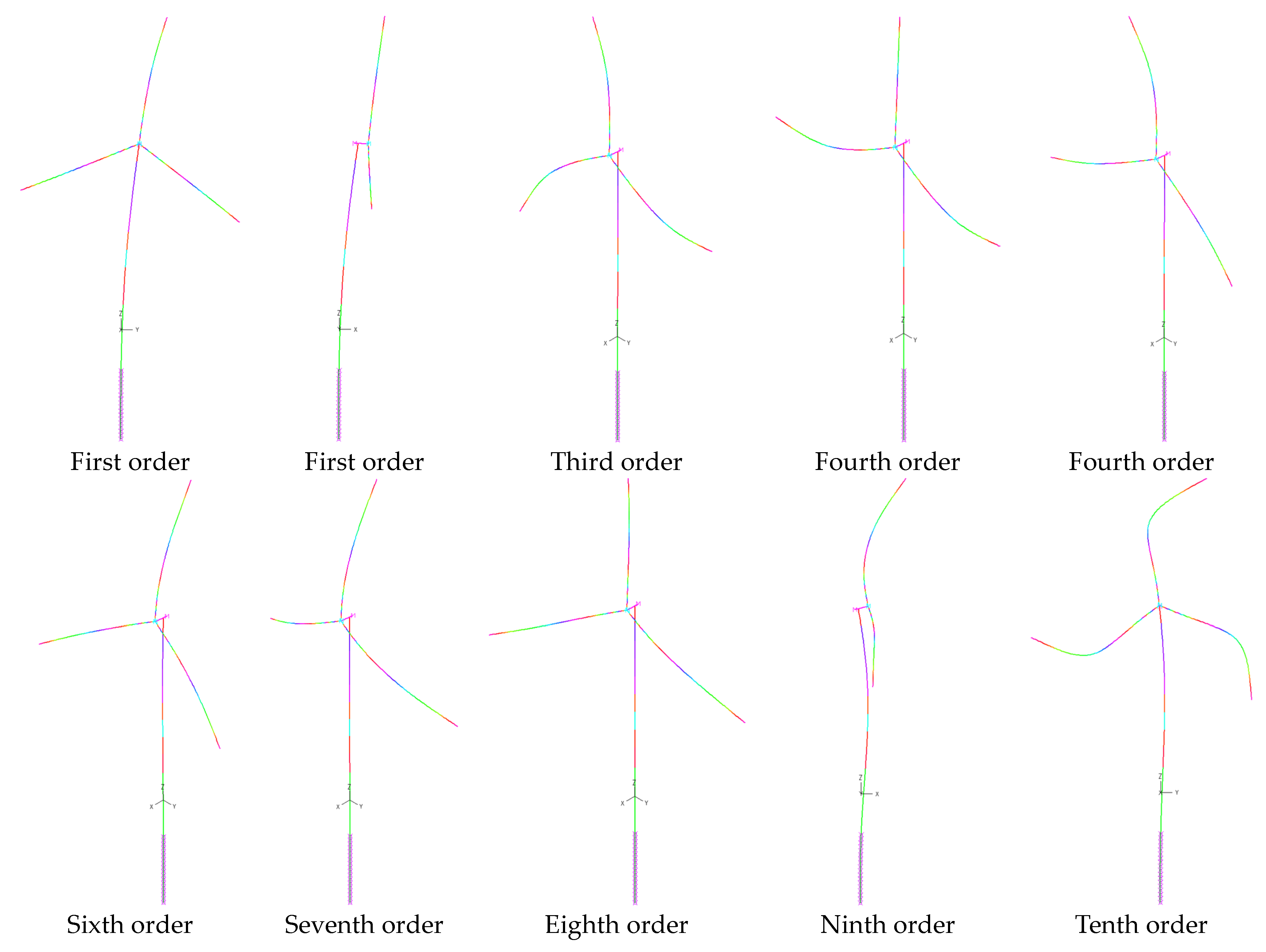
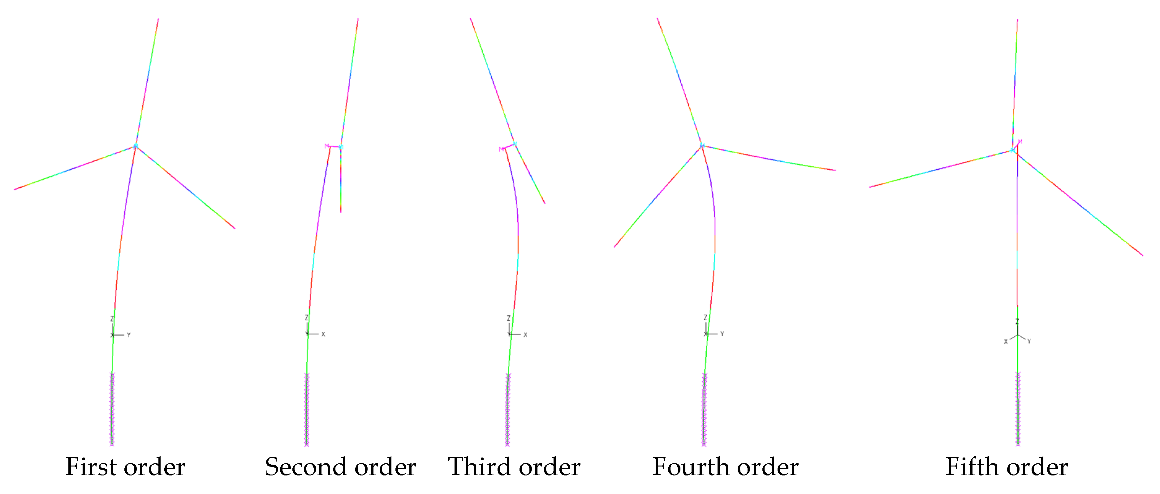
3.1. Dynamic Characteristic Analysis of the 5 MW and 10 MW MOWTs

In this section, the natural frequencies and mode shapes of 5 MW and 10 MW MOWTs were analyzed using the ‘Frequency/Modes’ module of ADINA.

Table 5. Full-system natural frequencies of the 5 MW MOWT.

Flexible Blade Model			Rigid Blade Model			Existing Result [48]
Mode	Frequency /Hz	Description	Mode	Frequency /Hz	Description	Mode	Frequency /Hz	Description
1	0.2474	1st Tower Side-to-Side	1	0.2479	1st Tower Side-to-Side	1	0.245	1st Tower Side-to-Side
2	0.2487	1st Tower Fore–Aft	2	0.2484	1st Tower Fore–Aft	2	0.247	1st Tower Fore–Aft
3	0.6451	1st Blade Asymmetric Edgewise	3	1.2384	2nd Tower Fore–Aft
4	0.6674	1st Blade Symmetric Edgewise	4	1.2818	2nd Tower Side-to-Side
5	0.6733	1st Blade Asymmetric Edgewise	5	1.4965	1st Tower Torsion
6	1.0189	1st Blade Asymmetric Flapwise
7	1.1191	1st Blade Symmetric Flapwise
8	1.1928	1st Tower Torsion
9	1.4092	2nd Tower Fore–Aft and 2nd Blade Asymmetric Edgewise
10	1.4665	2nd Tower Side-to-Side and 2nd Blade Asymmetric Flapwise

presents a subset of natural frequencies for the 5 MW MOWT using flexible blade and rigid blade models. The natural frequencies of the first two mode shapes obtained from the flexible blade model showed a high agreement with the existing research [48]. This indicates that the 5 MW MOWT model of this study provides a reliable representation. According to the table, the natural frequencies of the first two mode shapes derived from both rigid blade and flexible blade models exhibited disparities of less than 1%. Hence, the model simplifying the rotor–nacelle assembly as a rigid mass body can effectively predict the first- and second-mode natural frequencies of the full system.

According to Table 5, it is evident that the rigid blade model fails to accurately capture the modes primarily influenced by blade deformation, specifically the third, fourth, fifth, sixth, and seventh modes. This observation is further supported by a visual comparison of modes for the 5 MW MOWT, as depicted in Figure 7 and Figure 8. The rigid blade model exhibited a significant discrepancy in estimating the natural frequencies associated with higher-order modes. For instance, the first torsional mode of the tower was overestimated by 25%, while the second fore–aft and the second side-to-side tower modes were underestimated by 12% and 13%, respectively. The rigid blade model can only provide reliable predictions for the first two natural frequencies.

The natural frequencies of the 10 MW MOWT are compared in

Table 6. Full-system natural frequencies of the 10 MW MOWT.

Flexible Blade Model			Rigid Blade Model			Existing Result [49]
Mode	Frequency /Hz	Description	Mode	Frequency /Hz	Description	Mode	Frequency /Hz	Description
1	0.2138	1st Tower Side-to-side	1	0.2147	1st Tower Side-to-side	1	0.217	1st Tower Side-to-Side
2	0.2152	1st Tower Fore–Aft	2	0.2158	1st Tower Fore–Aft
3	0.4896	1st Blade Asymmetric Edgewise	3	1.0740	1st Tower Torsion
4	0.5078	1st Blade Symmetric Edgewise	4	1.1169	2nd Tower Fore–Aft
5	0.5138	1st Blade Asymmetric Edgewise	5	1.2096	2nd Tower Side-to-side
6	0.6811	1st Blade Asymmetric Flapwise
7	0.8331	1st Blade Symmetric Flapwise
8	0.9069	1st Tower Torsion
9	1.2496	2nd Tower Fore–Aft and 2nd Blade Asymmetric Edgewise
10	1.3817	2nd Tower Side-to-side and 2nd Blade Asymmetric Flapwise

, and the corresponding modes are illustrated in Figure 9 and Figure 10. The results of the flexible blade model closely match those in our previous study [49], with a relative error of less than 1.0%. The disparities between the flexible blade and rigid blade models showed similarities to those observed for the 5 MW MOWT. Specifically, the rigid blade model exhibited a 19% overestimation in the first torsional mode of the tower, while the second fore–aft and the second side-to-side tower modes of the tower were underestimated by 11% and 13%, respectively.

The natural frequencies of the first five modes of the full system using the rigid blade model are presented in

Table 7. Natural frequencies for the fore–aft tower modes.

5 MW MOWT				10 MW MOWT
Mode	Rigid (Hz)	Flexible (Hz)	Relative Difference (%)	Mode	Rigid (Hz)	Flexible (Hz)	Relative Difference (%)
1	0.2484	0.2487	−0.12	1	0.2158	0.2152	0.27
2	1.26	1.41	−10.01	2	1.12	1.25	−10.41
3	2.52	3.04	−17.11	3	2.2	2.96	−25.66
4	4.56	4.94	−8.33	4	3.91	4.87	−19.72
5	7.41	7.88	−6.34	5	6.27	7.04	−10.94

. For comparison, the natural frequencies of corresponding modes of the system using the flexible blade model are provided, along with the relative difference between them. It is important to note that the term ‘corresponding’ refers to the similarity in tower deflection shapes between the two models. From Table 7, it is evident that the flexible blade model predicts significantly different natural frequencies for higher tower modes in the fore–aft direction of wind turbines.

This section compares the variations in natural frequencies and mode shapes predicted by the flexible blade and rigid blade models of MOWTs. It can be concluded that the rigid flexibility has little influence on the natural frequencies of the first and second modes of the full system. However, the examination of higher-order modes and their natural frequencies reveals that blade flexibility significantly influences their natural frequencies.

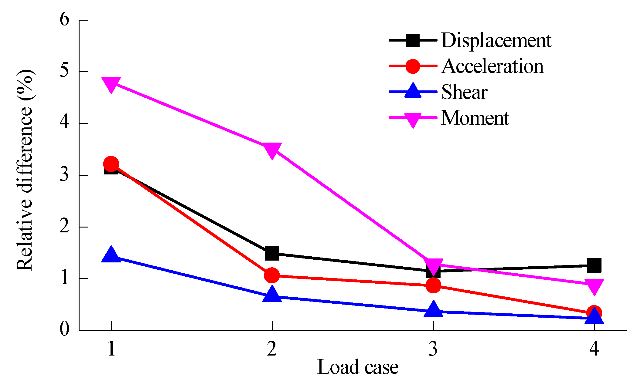
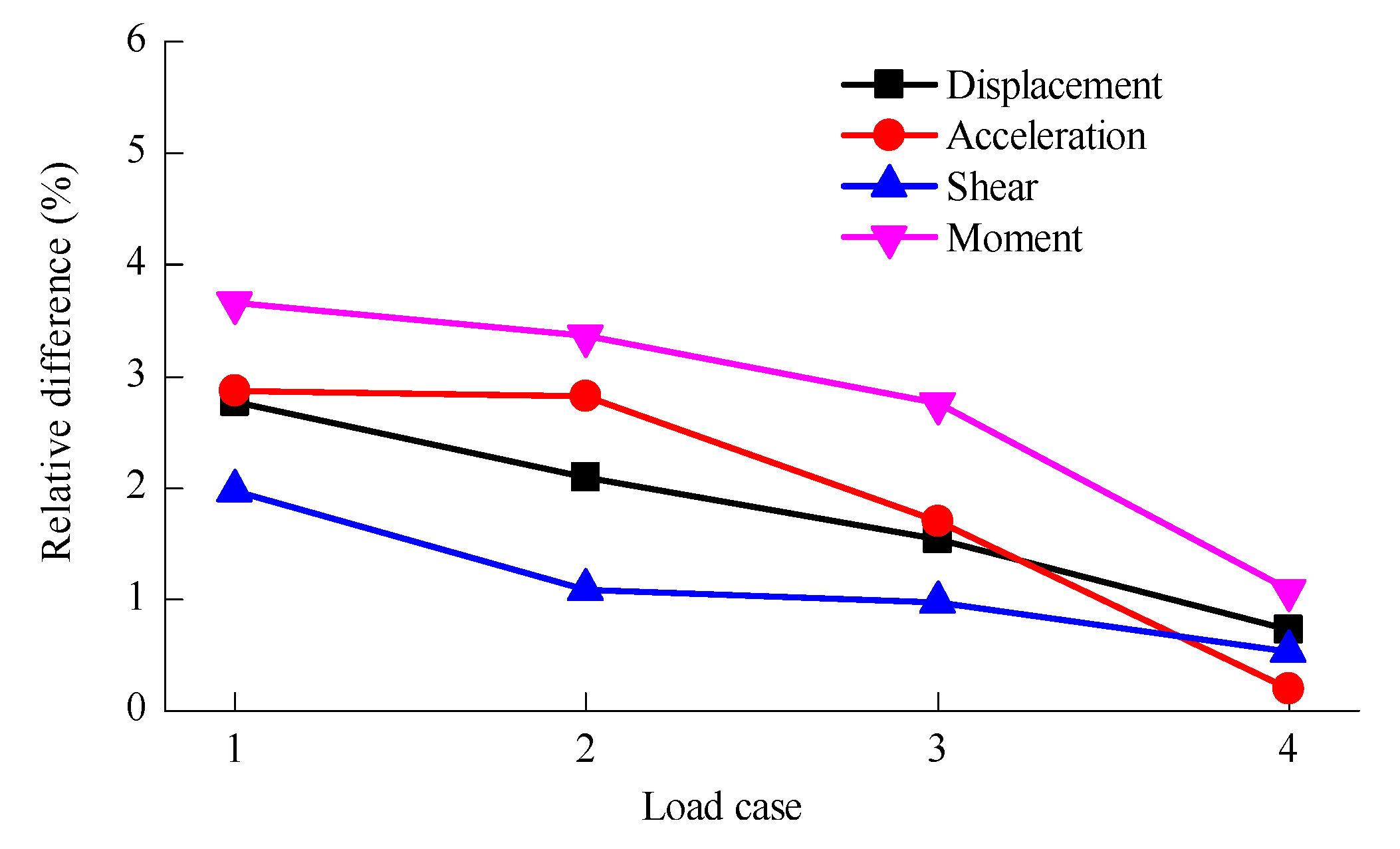
3.2. Dynamic Response of the 5 MW and 10 MW MOWTs Excited by Wave Load

For load case 1 of Table 2, Figure 11 depicts the time histories of tower-top acceleration and their Fourier amplitude spectra obtained from both the flexible and rigid blade models for the 5 MW MOWT. The tower-top accelerations obtained from these models exhibited a high degree of consistency in this load case. For MOWTs, wave loads are typically characterized as low-frequency excitations, resulting in the prevalence of low-order modes in the structural dynamic response. Furthermore, Figure 11b demonstrates that the tower-top acceleration was primarily characterized by low frequencies. Considering the satisfactory agreement between the two models in predicting the low-order dynamic characteristics of MOWTs, the prediction relative difference in the dynamic response of the system under wave excitations would be relatively minimal. In this context, the relative difference in the analysis results of the two models can be defined as

$$\mathsf{\delta }=\frac{\left|R_{\mathrm{r}}-R_{\mathrm{f}}\right|}{R_{\mathrm{f}}}\times 100\%$$

(9)

where R_f and R_r represent the response amplitude of MOWTs using the flexible blade model and rigid blade model, respectively. Figure 12 illustrates the relative difference in tower-top displacement, acceleration, mudline shear force, and bending moment obtained from both methods for the 5 MW MOWT. The maximum relative difference was less than 5%, indicating the high precision of the rigid blade model.

The discrepancies between the two models for the 10 MW MOWT were similarly insignificant. Figure 13 displays the time histories of tower-top acceleration and their corresponding Fourier amplitude spectra obtained from both models for the 10 MW MOWT. Furthermore, Figure 14 offers a comprehensive depiction of the relative difference in tower-top displacement, acceleration, mudline shear force, and bending moment obtained from both methods for the 10 MW MOWT. All of these relative differences were less than 4%, which reveals that the flexibility of the blade has a negligible influence on predicting the dynamic response of the 10 MW MOWT excited by the wave.

This section investigates the disparities in predicting the dynamic response of MOWTs under wave excitations using both the flexible blade and rigid blade models. The results indicate that the relative differences between the two models for the selected indicators of structural dynamic response were below 5%, which meets the engineering margin requirement. Given that wave loads are characterized as low-frequency excitations and that blade flexibility has minimal impact on the low-order modes of MOWTs, the influence of blade flexibility on the dynamic response of MOWTs under wave excitations is insignificant.

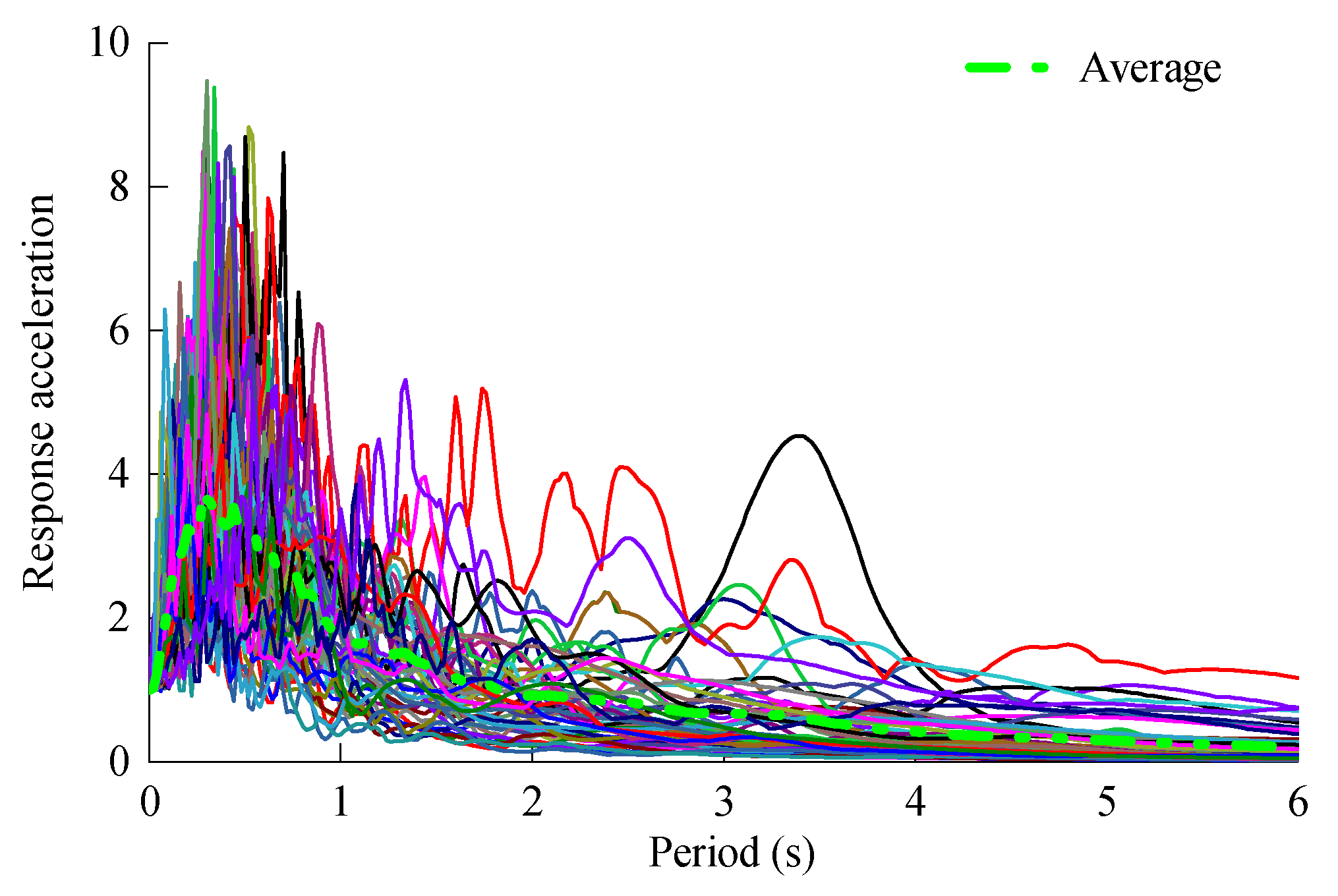
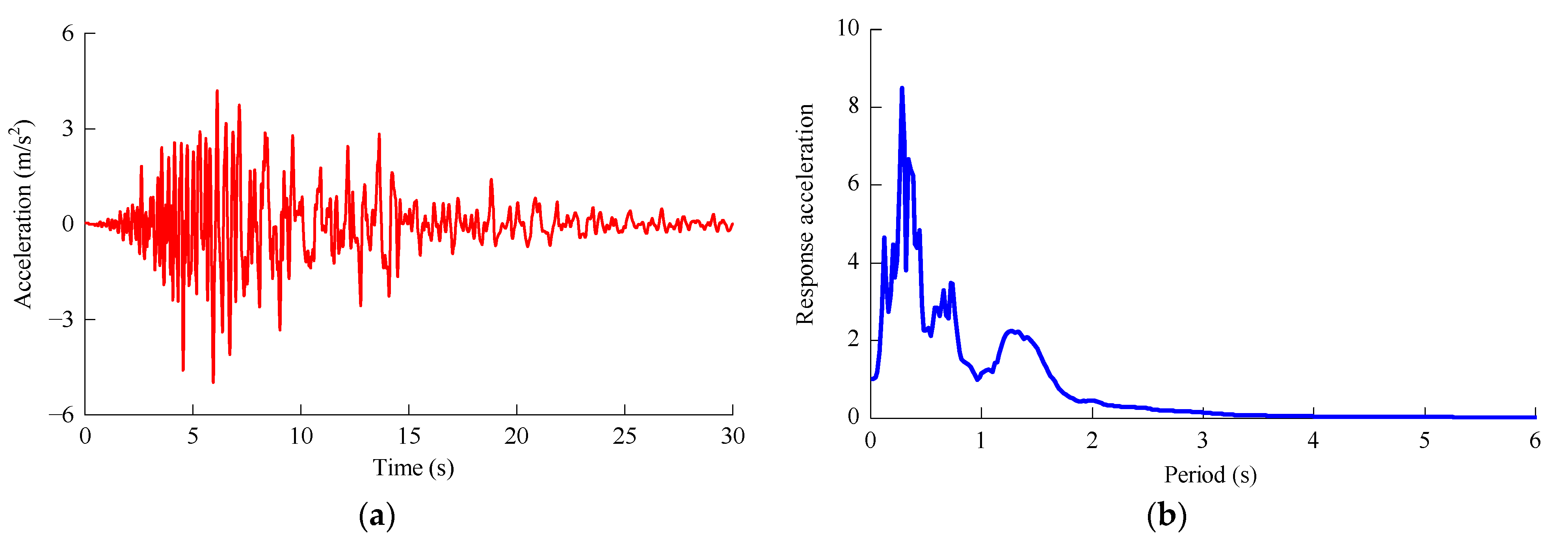
3.3. Seismic Response of 5 MW and 10 MW MOWTs

For these two MOWTs, the decay of free vibration suggests a damping ratio of approximately 1% for the first mode. Therefore, Figure 15 illustrates the response spectra of the seismic records listed in Table 3 with a damping ratio of 1%. In this context, the non-dimensional amplification factor response spectrum is utilized, which is calculated as follows:

$$\mathsf{\beta }\left(T\right)=\frac{S_{\mathrm{a}}}{a_{\max }}$$

(10)

where S_a represents the absolute acceleration response spectrum value of the seismic motion, while a_max denotes the corresponding peak acceleration. This collection of earthquake records covers a broad range of periods, with a particular focus on the period interval [0.06 s, 3.8 s], where the amplification factor response spectrum can exceed 3.0. This interval encompasses the first 40 or so mode shapes of the 5 MW and 10 MW MOWTs. Therefore, the use of this set of strong earthquake records to examine the disparities between the flexible blade and rigid blade models is representative.

Figure 16 depicts a horizontal acceleration time history recorded by the Bolu station during the 1999 Duzce earthquake in Turkey and the 1% damped response spectrum. The primary period of this seismic record is 0.32 s, which qualifies as high-frequency excitation for both wind turbines in this study. For the 5 MW MOWT, Figure 17 presents the tower-top acceleration time history and the corresponding Fourier amplitude spectrum obtained from both the flexible blade and rigid blade models. The peak acceleration of the nacelle for the flexible blade model was 4.84 m/s², while it was 6.47 m/s² for the rigid blade model, resulting in a relative difference of 33.8%. The Fourier amplitude spectra for the first mode of both models were 0.86 and 0.90, respectively, indicating minimal differences. However, for the second, third, and fourth modes of the tower, the Fourier spectra values obtained from the rigid blade model were significantly greater than those from the flexible blade model. According to the natural frequencies listed in Table 5 and the acceleration response spectrum in Figure 16b, the response spectrum value corresponding to the second mode of the tower in the rigid blade model was 0.60, whereas it was 0.43 in the flexible blade model. This discrepancy leads to a higher predicted peak acceleration of the nacelle from the rigid blade model compared to the flexible model.

For the 5 MW MOWT, Figure 18a illustrates the time history of the mudline bending moment of the monopile obtained from both the flexible blade and rigid blade models. The peak mudline bending moment for the flexible blade model was 123.5 MN·m, whereas it was 163.3 MN·m for the rigid blade model, resulting in a relative difference of 38.7%. To normalize the bending moment time history, the following formula was employed:

$$\overline{M}\left(t\right)=\frac{M\left(t\right)}{M_{\mathrm{fr},\max }}$$

(11)

where $\overline{M}\left(t\right)$ is the dimensionless bending moment time history, M(t) represents the tower bending moment time history, and M_fr,max is the maximum tower bending moment predicted by both the flexible blade and rigid blade models. The Fourier spectra of the dimensionless bending moment were analyzed and are presented in Figure 18b for both the flexible blade and rigid blade models of the 5 MW MOWT. The Fourier amplitude spectra for the first mode of both models were 0.238 and 0.24, respectively, indicating minimal difference. However, for the second tower mode, the Fourier spectra value obtained from the rigid blade model was significantly greater than that from the flexible blade model. Since the second tower mode is substantially excited in the rigid blade model, the mudline bending moment was higher compared to the flexible model.

For the 10 MW MOWT, Figure 19 depicts the tower-top acceleration time history and the corresponding Fourier amplitude spectrum obtained from both the flexible blade and rigid blade models. The peak acceleration of the nacelle was 5.95 m/s² for the flexible blade model, while it was 8.31 m/s² for the rigid blade model, resulting in a relative difference of 39.6%. Regarding the first four modes of the tower, the Fourier spectra values for the rigid blade model were significantly higher than those for the flexible blade model. Figure 20 displays the time history of the mudline bending moment and its Fourier amplitude spectrum for both the flexible blade and rigid blade models. The peak bending moment of the mudline was 278.7 MN·m for the flexible blade model, while it was 348.2 MN·m for the rigid blade model, resulting in a relative difference of 24.9%. In addition, it can be concluded that the Fourier spectra corresponding to the second mode of the rigid blade model were significantly greater than that of the flexible blade model according to Figure 20b.

Figure 21 presents a horizontal acceleration time history recorded by the Capitola station during the 1989 Loma Prieta earthquake and the 1% damped response spectrum. The dominant period of this seismic record is 0.28 s, which is also high-frequency excitation for these wind turbines. For the 5 MW MOWT, Figure 22 displays the tower-top acceleration time history and the corresponding Fourier amplitude spectrum obtained from both the flexible blade and rigid blade models. The peak acceleration of the nacelle was 6.59 m/s² for the flexible blade model, while it was 4.84 m/s² for the rigid blade model, resulting in a relative difference of −26.6%. In terms of the second mode of the system, the Fourier spectra value obtained from the flexible blade model was approximately 5 times that of the rigid blade model. Considering the natural frequencies listed in Table 5 and the acceleration response spectrum in Figure 21b, the response spectrum value corresponding to the second mode frequency of the tower was 0.95 for the rigid blade model and 0.51 for the flexible blade model. This disparity leads to a significantly higher predicted peak acceleration of the nacelle from the flexible blade model compared to the rigid model.

Figure 23a presents the time history of the mudline bending moment for the 5 MW MOWT obtained from both the flexible blade and rigid blade models. The flexible blade model predicts a maximum mudline bending moment of 167.9 MN·m, while the rigid blade model predicts a value of 102.1 MN·m, resulting in a relative difference of −39.3%. Additionally, Figure 23b illustrates the dimensionless Fourier amplitude spectra of the mudline bending moment, comparing the results obtained from both models. The spectra for the first mode were 0.0336 and 0.034, respectively, indicating a small difference. However, for the second tower mode, the flexible blade model exhibited significantly higher Fourier spectrum values compared to the rigid blade model. This discrepancy arises from the significant excitation of the second tower mode in the flexible blade model, resulting in a higher mudline bending moment compared to the prediction of the rigid blade model.

Figure 24 illustrates the tower-top acceleration time history and its Fourier amplitude spectra for the 10 MW MOWT, obtained from these two different analysis models. The peak nacelle acceleration was 5.41 m/s² for the flexible blade model, while the rigid blade model predicted a value of 6.86 m/s², resulting in a relative difference of 26.8%. The Fourier spectrum values for the third and fourth tower modes were significantly higher in the rigid blade model compared to the flexible blade model. In Figure 25a, the time history of the mudline bending moment is depicted for both the flexible blade and rigid blade models. The flexible blade model estimated a peak mudline bending moment of 207.3 MN·m, while the rigid blade model predicted a value of 162.1 MN·m, resulting in a relative difference of −21.8%. Figure 25b displays the dimensionless Fourier amplitude spectra of the mudline bending moment for the 10 MW MOWT. Obviously, the Fourier spectra value corresponding to the second tower mode was significantly higher in the flexible blade model compared to the rigid blade model.

The rigid blade model fails to adequately capture the dynamic characteristics of these two MOWTs, including higher-order natural frequencies and modes. Additionally, the low damping exhibited by the MOWT in the parked state exacerbates the oscillation of the acceleration response spectra. As a result, when subjected to seismic excitation, the rigid blade model is prone to significant inaccuracies in predicting the dynamic response of the OWTs. Specifically, for the same MOWT and input seismic motion, the rigid blade model may significantly overestimate or underestimate various system response parameters. For example, this includes the tower-top acceleration and mudline bending moment of the 10 MW MOWT when exposed to the Capitola seismic record.

In seismic load cases, the relative difference in the seismic response of MOWTs caused by the overestimation or underestimation of the rigid blade model can be defined as follows:

$${\mathsf{\delta }}_E=\frac{R_{\mathrm{E},\mathrm{r}}-R_{\mathrm{E},\mathrm{f}}}{R_{\mathrm{E},\mathrm{f}}}\times 100\%$$

(12)

where $R_{\mathrm{E},\mathrm{f}}$ represents the peak response obtained from the flexible blade model under seismic excitation and $R_{\mathrm{E},\mathrm{r}}$ represents the peak response obtained from the rigid blade model under seismic excitation. Figure 26 depicts the relative difference in nacelle acceleration predicted by the rigid blade model for both the 5 MW and 10 MW MOWTs when subjected to the seismic motions listed in Table 3. For the 5 MW MOWT, 29 seismic excitations resulted in a nacelle acceleration relative difference that exceeded the range of [−15%, 15%]. Similarly, for the 10 MW turbine, this number was 26. Figure 27 illustrates the relative difference in the mudline bending moment predicted by the rigid blade model for both turbines. In the case of the 5 MW MOWT, 31 seismic excitations led to a peak mudline bending moment relative difference beyond the range of [−15%, 15%], while for the 10 MW turbine, this number was 28. Considering the precision requirements in seismic engineering, models with relative differences exceeding 15% should be improved to enhance accuracy. Hence, the flexibility of the blades may have a noteworthy impact on the seismic response of MOWTs.

If the rigid blade model is used due to a lack of stiffness data of the blades, it is crucial that it undergo a comprehensive model verification process. This verification should include parameters that have an impact on the safety of the turbine and support structures. Additionally, selecting an adequate number of seismic motions is essential to minimize the possibility of incorrect outcomes. For example, Figure 28 demonstrates the difference in nacelle displacement predicted by the rigid blade model for the aforementioned two MOWTs. If only a subset of seismic motions from Table 3 is considered, focusing solely on nacelle displacement response, it may lead to an improper conclusion regarding the suitability of the rigid model for predicting the seismic response of these two MOWTs.

4. Conclusions and Outlook

It is usually difficult to obtain the structural properties of blades for commercial wind turbines. In this circumstance, the flexibility of blades is neglected, and the rotor is simplified as a rigid body. This study examined the structural models of the 5 MW and DTU 10 MW MOWTs considering flexible blade and rigid blade configurations. The discrepancies in predicting natural frequencies and modes between these two models were analyzed, and the differences in the dynamic response of wind turbines under wave and seismic excitations were evaluated. Based on these findings, the following conclusions can be drawn:

• The rigid blade model failed to account for the flexible deformation of the blades, which led to the exclusion of blade-deformation-dominated modes when determining the system modes. Moreover, it introduced significant differences when calculating the higher-order natural frequencies. For instance, the frequency of the second fore–aft tower mode for the 5 MW and 10 MW MOWTs was underestimated by 12% and 13%, respectively. Therefore, the flexibility of the blades can have a remarkable impact on the higher-order modes and natural frequencies of MOWTs.
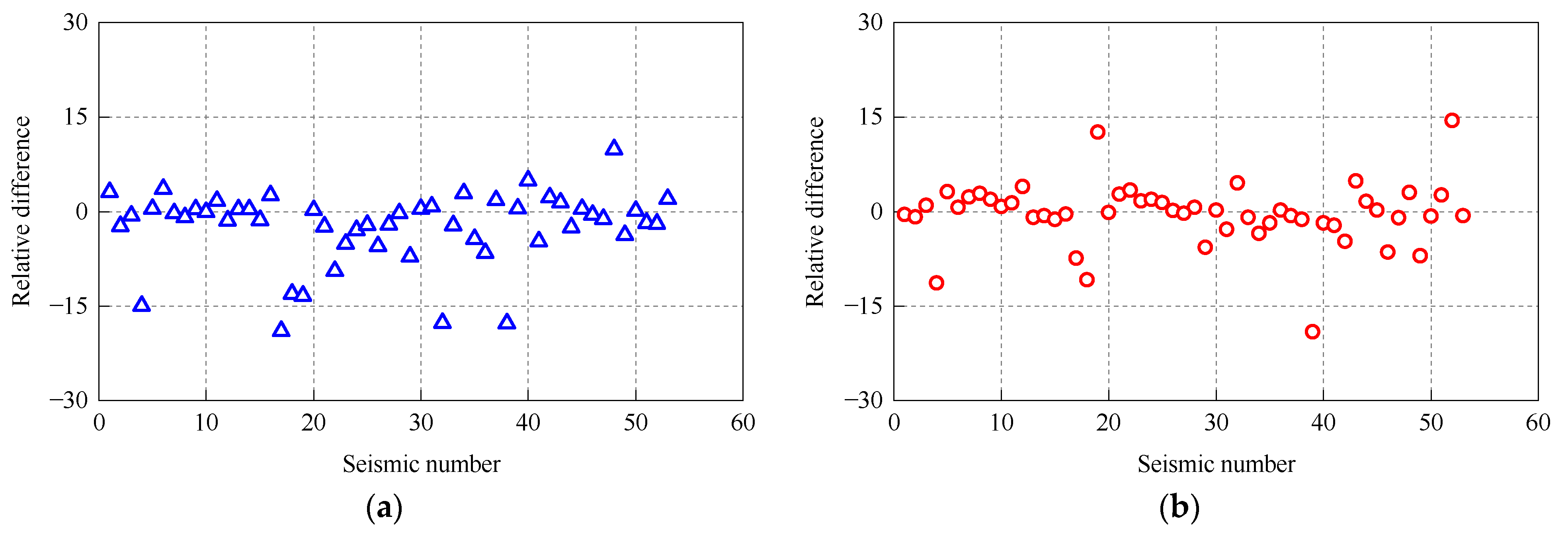
• The dynamic response of both MOWTs under wave excitations was mainly governed by the first tower mode, with the blade flexibility having a minimal influence. The rigid blade model effectively predicted the deformation and internal forces of the supported structure of MOWTs in this load case. Taking nacelle acceleration and the mudline bending moment, for example, the maximum discrepancy between the rigid and flexible blade models was less than 5%. Hence, the flexibility of the blades has a negligible impact on the dynamic response of MOWTs solely excited by waves.
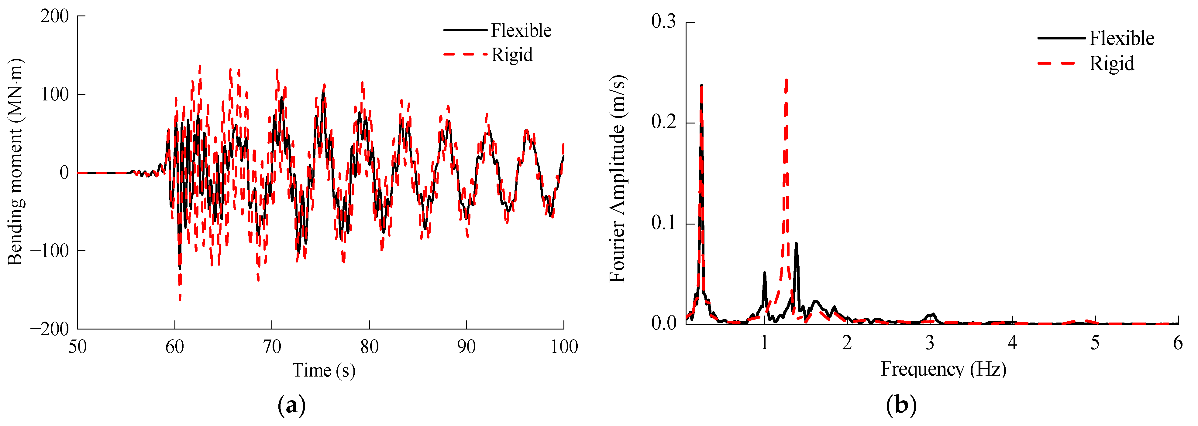
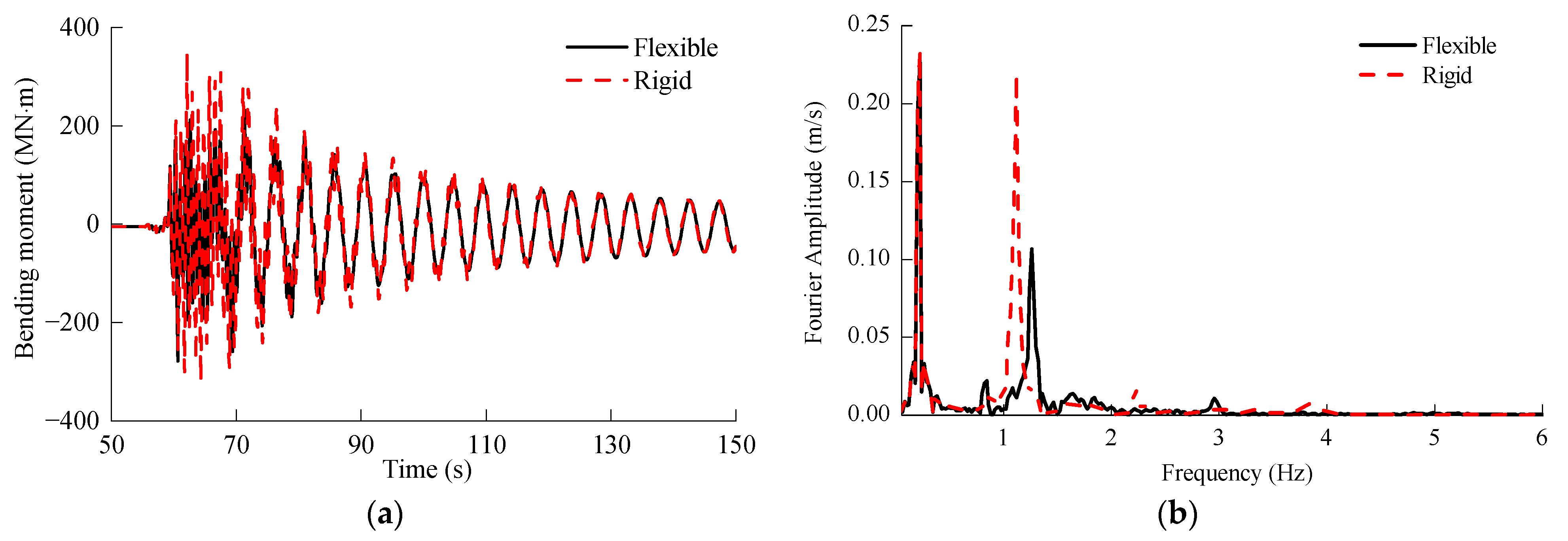
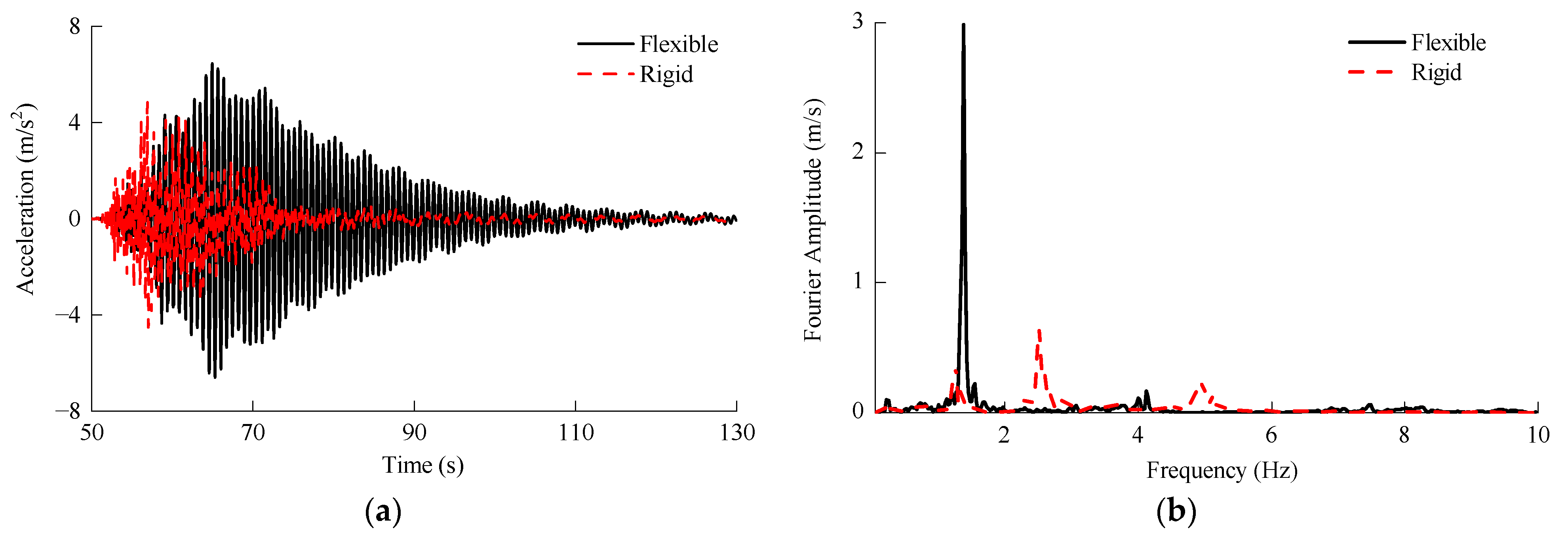
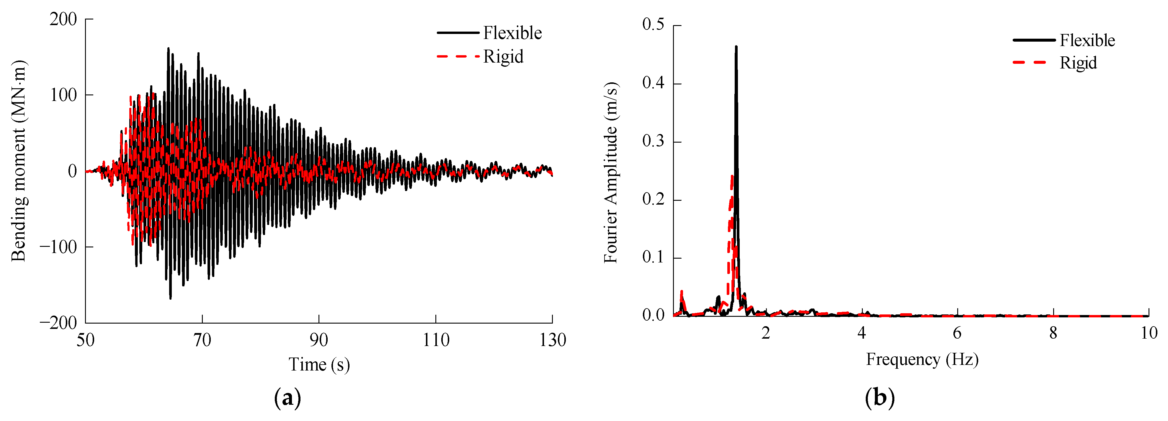
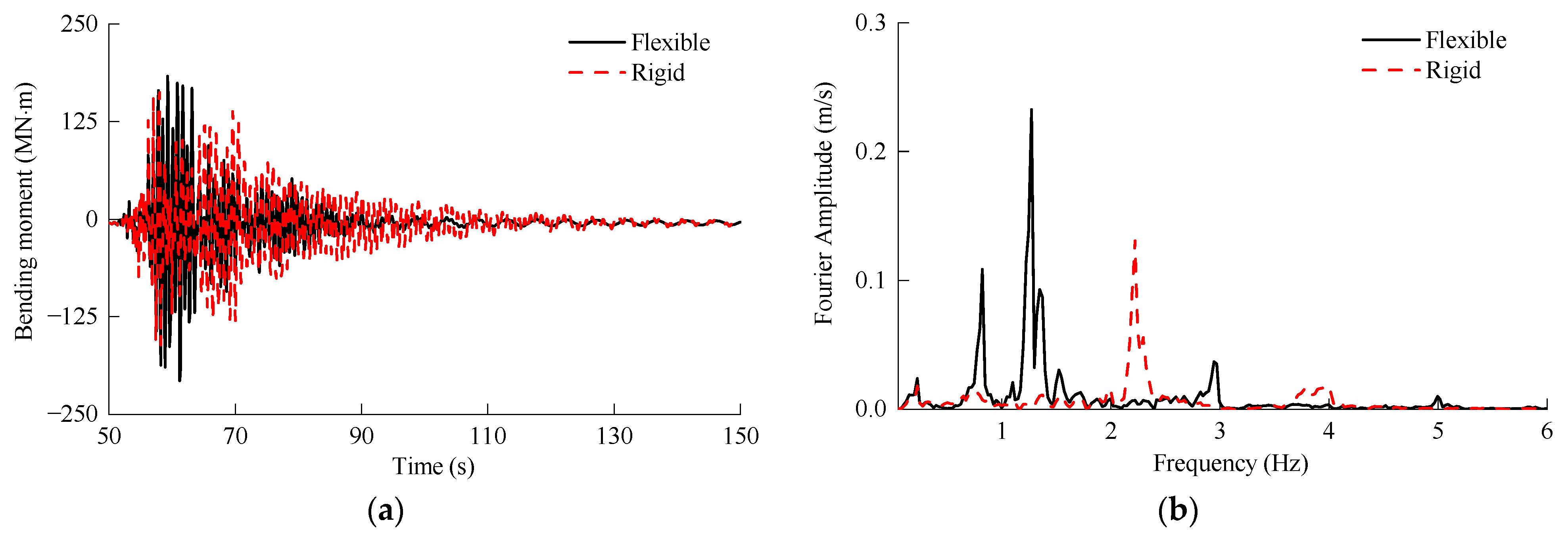
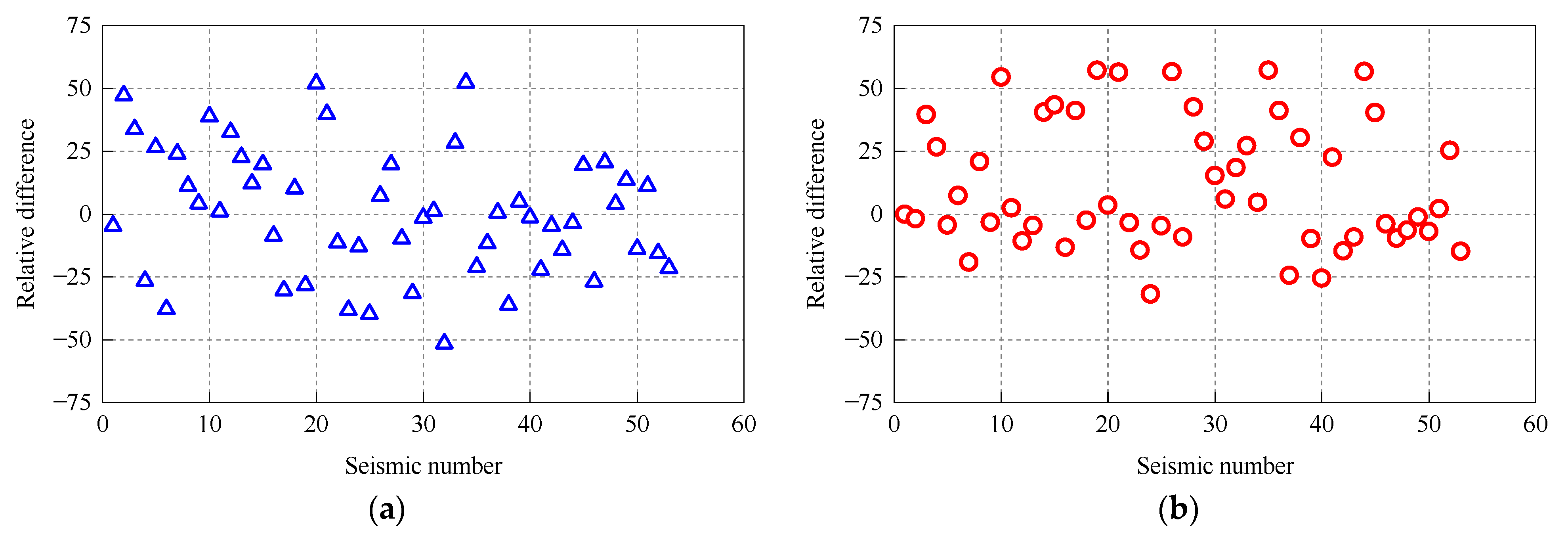
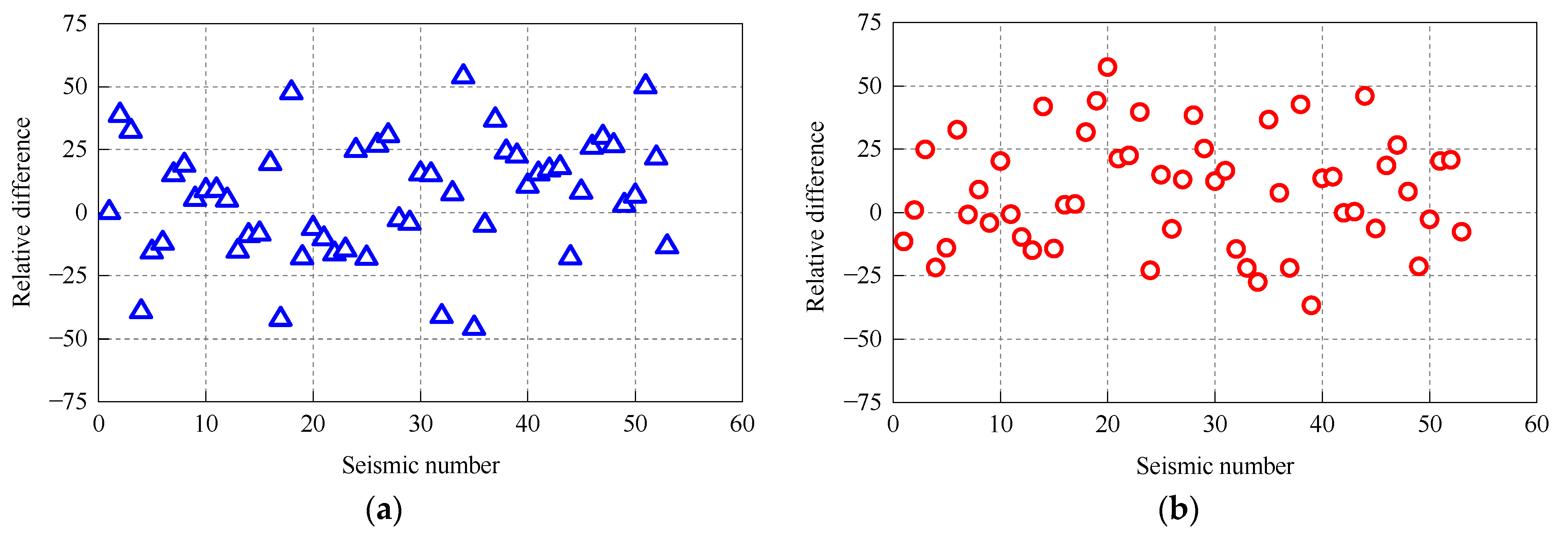
• The seismic excitation generally consists of rich high-frequency components that strongly stimulate higher-order tower modes. As a result, the rigid blade model tended to substantially underestimate or overestimate the peak seismic response of these two MOWTs. For example, in terms of nacelle acceleration and the mudline bending moment, the maximum relative difference between the rigid blade and flexible blade model exceeded 50%. Therefore, blade flexibility has a notable influence on the seismic response of MOWTs.

Based on the aforementioned conclusions, several modeling requirements of blades for the dynamic analysis of MOWTs can be identified. When analyzing the low-order modes and dynamic responses of OWTs under wave excitations, the influence of blade flexibility can be neglected. The rotor can be simplified as a lumped mass, requiring only its total mass and moment of inertia. However, when analyzing the high-order modes and dynamic response of OWTs under seismic excitations, it is necessary to consider the flexibility of blades. In this situation, the structural model should, at minimum, accurately represent the distribution characteristics of blade mass and stiffness. Although these conclusions and prospects are based on the numerical simulations conducted in this study, relevant experimental research and theoretical analyses can also draw inspiration from them.

References

1. Subbulakshmi, A.; Verma, M.; Keerthana, M.; Sasmal, S.; Harikrishna, P.; Kapuria, S. Recent advances in experimental and numerical methods for dynamic analysis of floating offshore wind turbines-an integrated review. Renew. Sustain. Energy Rev. 2022, 164, 112525. [Google Scholar] [CrossRef]
2. GWEC. Global Wind Report: Annual Market Update 2022. Global Wind Energy Council. 2023. Available online: https://gwec.net/wp-content/uploads/2020/04/GWEC-Global-Wind-Report-2019.pdf (accessed on 20 July 2023).
3. Veers, P.S.; Dykes, K.; Lantz, E.; Barth, S.; Bottasso, C.L.; Carlson, O.; Clifton, A.; Green, J.; Green, P.; Holttinen, H.; et al. Grand challenges in the science of wind energy. Science 2019, 366, eaau2027. [Google Scholar] [CrossRef] [PubMed]
4. Yeter, B.; Garbatov, Y. Structural integrity assessment of fixed support structures for offshore wind turbines: A review. Ocean Eng. 2022, 244, 110271. [Google Scholar] [CrossRef]
5. Wang, W.; Li, X.; Pan, Z.; Zhao, Z. Motion control of pentapod offshore wind turbines under earthquakes by tuned mass damper. J. Mar. Sci. Eng. 2020, 7, 224. [Google Scholar] [CrossRef]
6. Jahani, K.; Langlois, R.G.; Afagh, F.F. Structural dynamics of offshore wind turbines: A review. Ocean Eng. 2022, 251, 111136. [Google Scholar] [CrossRef]
7. Leng, D.; Yang, Y.; Xu, K.; Li, Y.; Xie, Y. Vibration control of offshore wind turbine under multiple hazards using single variable-stiffness tuned mass damper. Ocean Eng. 2021, 236, 109473. [Google Scholar] [CrossRef]
8. Ko, Y.-Y.; Li, Y.-T. Response of a scale-model pile group for a jacket foundation of an offshore wind turbine in liquefiable ground during shaking table tests. Earthq. Eng. Struct. Dyn. 2020, 49, 1682–1701. [Google Scholar] [CrossRef]
9. Manwell, J.F.; McGowan, J.G.; Rogers, A.L. Wind Energy Explained: Theory, Design and Application, 2nd ed.; Wiley: Sussex, UK, 2010. [Google Scholar]
10. Failla, G.; Santangelo, F.; Foti, G.; Scali, F.; Arena, F. Response-spectrum uncoupled analyses for seismic assessment of offshore wind turbines. J. Mar. Sci. Eng. 2018, 6, 85. [Google Scholar] [CrossRef]
11. Zhao, Z.; Dai, K.; Lalonde, E.R.; Meng, J.; Li, B.; Ding, Z.; Bitsuamlak, G. Studies on application of scissor-jack braced viscous damper system in wind turbines under seismic and wind loads. Eng. Struct. 2019, 196, 109294. [Google Scholar] [CrossRef]
12. Fan, J.; Li, Q.; Zhang, Y. Collapse analysis of wind turbine tower under the coupled effects of wind and near-field earthquake. Wind Energy 2019, 22, 407–419. [Google Scholar] [CrossRef]
13. Santangelo, F.; Failla, G.; Arena, F.; Ruzzo, C. On time-domain uncoupled analyses for offshore wind turbines under seismic loads. Bull. Earthq. Eng. 2018, 16, 1007–1040. [Google Scholar] [CrossRef]
14. Zuo, H.; Bi, K.; Hao, H. Dynamic analyses of operating offshore wind turbines including soil-structure interaction. Eng. Struct. 2018, 157, 42–62. [Google Scholar] [CrossRef]
15. Zuo, H.; Bi, K.; Hao, H.; Xin, Y.; Li, J.; Li, C. Fragility analyses of offshore wind turbines subjected to aerodynamic and sea wave loadings. Renew. Energy 2020, 160, 1269–1282. [Google Scholar] [CrossRef]
16. Ali, A.; Risi, R.D.; Sextos, A. Finite element modeling optimization of wind turbine blades from an earthquake engineering perspective. Eng. Struct. 2020, 222, 111105. [Google Scholar] [CrossRef]
17. Huang, H.S. Simulations of 10mw wind turbine under seismic loadings. Compos. Struct. 2022, 279, 114686. [Google Scholar] [CrossRef]
18. Bazeos, N.; Hatzigeorgiou, G.D.; Hondros, I.D.; Karamaneas, H.; Karabalis, D.L.; Beskos, D.E. Static, seismic and stability analyses of a prototype wind turbine steel tower. Eng. Struct. 2002, 24, 1015–1025. [Google Scholar] [CrossRef]
19. Lavassas, I.; Nikolaidis, G.; Zervas, P.; Efthimiou, E.; Doudoumis, I.; Baniotopoulos, C. Analysis and design of the prototype of a steel 1-MW wind turbine tower. Eng. Struct. 2003, 25, 1097–1106. [Google Scholar] [CrossRef]
20. Martinez-Vazquez, P.; Gkantou, M.; Baniotopoulos, C. Strength demands of tall wind turbines subject to earthquakes and wind load. Procedia Eng. 2017, 199, 3212–3217. [Google Scholar] [CrossRef]
21. Hansen, M.O.L.; Sørensen, J.N.; Voutsinas, S.; Sørensen, N.; Madsen, H.A. State of the art in wind turbine aerodynamics and aero-elasticity. Prog. Aerosp. Sci. 2006, 42, 285–330. [Google Scholar] [CrossRef]
22. Dong, W.; Moan, T.; Gao, Z. Long-term fatigue analysis of multi-planar tubular joints for jacket-type offshore wind turbine in time domain. Eng. Struct. 2011, 33, 2002–2014. [Google Scholar] [CrossRef]
23. Abhinav, K.A.; Saha, N. Coupled hydrodynamic and geotechnical analysis of jacket offshore wind turbine. Soil Dyn. Earthq. Eng. 2015, 73, 66–79. [Google Scholar] [CrossRef]
24. Taflanidis, A.A.; Loukogeorgaki, E.; Angelides, D.C. Offshore wind turbine risk quantification/evaluation under extreme environmental conditions. Reliab. Eng. Syst. Saf. 2013, 115, 19–32. [Google Scholar] [CrossRef]
25. Jiang, W.; Lin, C.; Sun, M. Seismic responses of monopile-supported offshore wind turbines in soft clays under scoured conditions. Soil Dyn. Earthq. Eng. 2021, 142, 106549. [Google Scholar] [CrossRef]
26. Yeh, P.H.; Chung, S.H.; Chen, B.F. Multiple TLDs on motion reduction control of the offshore wind turbines. J. Mar. Sci. Eng. 2020, 8, 470. [Google Scholar] [CrossRef]
27. Jalbi, S.; Nikitas, G.; Bhattacharya, S.; Alexander, N. Dynamic design considerations for offshore wind turbine jackets supported on multiple foundations. Mar. Struct. 2019, 67, 102631. [Google Scholar] [CrossRef]
28. Feyzollahzadeh, M.; Mahmoodi, M.J.; Yadavar-Nikravesh, S.M.; Jamali, J. Wind load response of offshore wind turbine towers with fixed monopile platform. J. Wind. Eng. Ind. Aerodyn. 2016, 158, 122–138. [Google Scholar] [CrossRef]
29. Wang, X.; Zeng, X.; Yang, X.; Li, J. Seismic response of offshore wind turbine with hybrid monopile foundation based on centrifuge modelling. Appl. Energy 2019, 235, 1335–1350. [Google Scholar] [CrossRef]
30. Wang, P.; Zhao, M.; Du, X.; Liu, J.; Xu, C. Wind, wave and earthquake responses of offshore wind turbine on monopile foundation in clay. Soil Dyn. Earthq. Eng. 2018, 113, 47–57. [Google Scholar] [CrossRef]
31. Yu, D.O.; Kwon, O.J. Predicting wind turbine blade loads and aeroelastic response using a coupled CFD-CSD method. Renew. Energy 2014, 70, 184–196. [Google Scholar] [CrossRef]
32. Bayati, I.; Belloli, M.; Bernini, L.; Zasso, A. Aerodynamic design methodology for wind tunnel tests of wind turbine rotors. J. Wind. Eng. Ind. Aerodyn. 2017, 167, 217–227. [Google Scholar] [CrossRef]
33. Arany, L.; Bhattacharya, S.; Macdonald, J.H.G.; Hogan, S.J. Closed form solution of eigen frequency of monopile supported offshore wind turbines in deeper waters incorporating stiffness of substructure and ssi. Soil Dyn. Earthq. Eng. 2016, 83, 18–32. [Google Scholar] [CrossRef]
34. Jonkman, J.; Butterfield, S.; Musial, W.; Scott, G. Definition of a 5-MW Reference Wind Turbine for Offshore System Development; National Renewable Energy Laboratory: Golden, CO, USA, 2009. Available online: https://www.osti.gov/biblio/947422 (accessed on 1 July 2023).
35. Bak, C.; Zahle, F.; Bitsche, R.; Kim, T.; Yde, A.; Henriksen, L.C.; Hansen, M.H.; Blasques, J.P.A.A.; Gaunaa, M.; Natarajan, A. Description of the DTU 10-MW reference wind turbine; DTU Wind Energy: Frederiksborgvej, Roskilde, Denmark, 2013; Available online: https://orbit.dtu.dk/files/55645274/The_DTU_10MW_Reference_Turbine_Christian_Bak.pdf (accessed on 1 July 2023).
36. Lee, J.W.; Lee, J.S.; Han, J.H.; Shin, H.K. Aeroelastic analysis of wind turbine blades based on modified strip theory. J. Wind. Eng. Ind. Aerodyn. 2012, 110, 62–69. [Google Scholar] [CrossRef]
37. Tran, T.T.; Kim, D.H. The coupled dynamic response computation for a semi-submersible platform of floating offshore wind turbine. J. Wind. Eng. Ind. Aerodyn. 2015, 147, 104–119. [Google Scholar] [CrossRef]
38. Meng, H.; Jin, D.; Li, L.; Liu, Y. Analytical and numerical study on centrifugal stiffening effect for large rotating wind turbine blade based on NREL 5MW and WindPACT 1. 5MW models. Renew. Energy 2022, 183, 321–329. [Google Scholar] [CrossRef]
39. DNV. Design of Offshore Wind Turbine Structures; Det Norske Veritas: Bærum, Norway, 2013. [Google Scholar]
40. Fischer, T.; De Vries, W.E.; Schmidt, B. UpWind design basis WP4: Offshore foundations and support structures; EU UpWind project: Stuttgart, Germany, 2010; Available online: https://repository.tudelft.nl/islandora/object/uuid:a176334d-6391-4821-8c5f-9c91b6b32a27/datastream/OBJ/download (accessed on 1 July 2023).
41. ATC. Quantification of Building Seismic Performance Factors; Report No FEMA-P695; Applied Technology Council: Redwood City, CA, USA, 2009. [Google Scholar]
42. ADINA. ADINA Theory and Modeling Guide; ADINA R&D Inc.: Watertown, MA, USA, 2014. [Google Scholar]
43. Bossanyi, E.A. Bladed for Windows User Manual; Garrad Hassan and Partners: Bristol, UK, 2016. [Google Scholar]
44. Sun, Y.L.; Xu, C.S.; Du, X.L.; Du, X.P.; Xi, R.Q. A modified p-y curve model of large-monopiles of offshore wind power plants. Eng. Mech. 2020, 8, 44–53. [Google Scholar] [CrossRef]
45. Kim, K.T.; Bathe, K.J. The Bathe subspace iteration method enriched by turning vectors. Comput. Struct. 2017, 186, 11–21. [Google Scholar] [CrossRef]
46. Makris, N.; Gazetas, G. Dynamic pile-soil-pile interaction. Part II: Lateral and seismic response. Earthq. Eng. Struct. Dyn. 1992, 21, 145–162. [Google Scholar] [CrossRef]
47. Xi, R.Q.; Xu, C.S.; Du, X.L.; Naggar, M.H.; Wang, P.G.; Liu, L.; Zhai, E.D. Framework for dynamic response analysis of monopile supported offshore wind turbine excited by combined wind-wave-earthquake loading. Ocean Eng. 2022, 247, 110743. [Google Scholar] [CrossRef]
48. Yang, Y.; Li, C.; Bashir, M.; Wang, J.; Yang, C. Investigation on the sensitivity of flexible foundation models of an offshore wind turbine under earthquake loadings. Eng. Struct. 2019, 183, 756–769. [Google Scholar] [CrossRef]
49. Xi, R.Q.; Wang, P.G.; Du, X.L.; Xu, C.S. Dynamic analysis of 10 MW monopile supported offshore wind turbine based on fully coupled model. Ocean Eng. 2021, 234, 109346. [Google Scholar] [CrossRef]
Figure 1. Structure of the blade.
Jmse 11 02041 g001
Figure 2. Mass distribution of the blade: (a) NREL 5 MW; (b) DTU 10 MW.
Jmse 11 02041 g002
Figure 3. Stiffness distribution of the blade: (a) NREL 5 MW; (b) DTU 10 MW.
Jmse 11 02041 g003
Figure 4. Soil profile of a typical marine site.
Jmse 11 02041 g004
Figure 5. Seismic response of the 5 MW MOWT: (a) displacement of the blade tip; (b) tower-top acceleration.
Jmse 11 02041 g005
Figure 6. Seismic response of the 10 MW MOWT: (a) displacement of the blade tip; (b) tower-top acceleration.
Jmse 11 02041 g006
Figure 7. First ten mode shapes of the 5 MW MOWT using the flexible blade model.
Jmse 11 02041 g007
Figure 8. First five mode shapes of 5 MW MOWT using the rigid blade model.
Jmse 11 02041 g008
Figure 9. First ten mode shapes of the 10 MW MOWT using the flexible blade model.
Jmse 11 02041 g009
Figure 10. First five mode shapes of the 10 MW MOWT using the rigid blade model.
Jmse 11 02041 g010
Figure 11. Nacelle response of the 5 MW MOWT using the flexible and rigid blade models: (a) nacelle acceleration time history; (b) nacelle Fourier amplitude.
Jmse 11 02041 g011
Figure 12. Response difference of the 5 MW MOWT between the flexible and rigid blade models.
Jmse 11 02041 g012
Figure 13. Nacelle response of the 10 MW MOWT using the flexible and rigid blade models: (a) nacelle acceleration time history; (b) nacelle Fourier amplitude.
Jmse 11 02041 g013
Figure 14. Response difference of the 10 MW MOWT between the flexible and rigid blade models.
Jmse 11 02041 g014
Figure 15. Non-dimensional response acceleration of input ground motion (the solid lines represent the response spectra of different seismic records).
Jmse 11 02041 g015
Figure 16. Bolu record of the 1999 Duzce earthquake in Turkey: (a) acceleration time history; (b) non-dimensional response acceleration.
Jmse 11 02041 g016
Figure 17. Nacelle acceleration of 5 MW MOWT excited by the Bolu record: (a) nacelle acceleration time history; (b) Fourier amplitude spectra.
Jmse 11 02041 g017
Figure 18. Mudline bending moment of the 5 MW MOWT excited by the Bolu record: (a) mudline bending moment of the monopile; (b) Fourier amplitude spectra.
Jmse 11 02041 g018
Figure 19. Nacelle acceleration of the 10 MW MOWT excited by the Bolu record: (a) nacelle acceleration time history; (b) Fourier amplitude spectra.
Jmse 11 02041 g019
Figure 20. Mudline bending moment of the 10 MW MOWT excited by the Bolu record: (a) mudline bending moment of the monopile; (b) Fourier amplitude spectra.
Jmse 11 02041 g020
Figure 21. Capitola record of the 1989 Loma Prieta earthquake: (a) acceleration time history; (b) non-dimensional response acceleration.
Jmse 11 02041 g021
Figure 22. Nacelle acceleration of the 5 MW MOWT excited by Capitola record: (a) nacelle acceleration time history; (b) Fourier amplitude spectra.
Jmse 11 02041 g022
Figure 23. Mudline bending moment of the 5 MW MOWT excited by the Capitola record: (a) mudline bending moment of the monopile; (b) Fourier amplitude spectra.
Jmse 11 02041 g023
Figure 24. Nacelle acceleration of the 10 MW MOWT excited by the Capitola record: (a) nacelle acceleration time history; (b) Fourier amplitude spectra.
Jmse 11 02041 g024
Figure 25. Mudline bending moment of the 10 MW MOWT excited by the Capitola record: (a) mudline bending moment of the monopile; (b) Fourier amplitude spectra.
Jmse 11 02041 g025
Figure 26. Relative difference in nacelle peak acceleration: (a) error for the 5 MW MOWT; (b) error for the 10 MW MOWT.
Jmse 11 02041 g026
Figure 27. Relative difference of the mudline bending moment: (a) error for the 5 MW MOWT; (b) error for the 10 MW MOWT.
Jmse 11 02041 g027
Figure 28. Relative error of nacelle displacement: (a) error for the 5 MW MOWT; (b) error for the 10 MW MOWT.
Jmse 11 02041 g028