Abstract
Automatic identification system (AIS) data record a ship’s position, speed over ground (SOG), course over ground (COG), and other behavioral attributes at specific time intervals during a ship’s voyage. At present, there are few studies in the literature on ship trajectory classification, especially the clustering of trajectory segments, to measure the multi-dimensional information of trajectories. Therefore, it is necessary to fully utilize the multi-dimensional information from AIS data when utilizing ship trajectory classification methods. Here, we propose a ship trajectory classification method based on multi-attribute trajectory similarity metrics which utilizes the following steps: (1) Improve the Douglas–Peucker (DP) algorithm by considering the SOG and COG; (2) use a multi-attribute symmetric segmentation path distance (MSSPD) for the similarity metric between trajectories; (3) cluster the segmented sub-trajectories based on the density-based spatial clustering of applications with noise (DBSCAN) algorithm; (4) adaptively determinate the optimal input parameters based on the proposed comprehensive clustering performance metrics. The proposed method was tested on real AIS data from Bohai Sea waters, and the experimental results show that the algorithm can accurately cluster the ship trajectory groups and extract traffic distributions in key waters.
1. Introduction
1.1. Background
Since 2002, the International Convention for the Safety of Life at Sea (SOLAS) has made AIS equipment mandatory for all international ships of more than 300 gross tons, non-international ships of less than 500 gross tons, and all passenger ships on international voyages [1]. This allows maritime authorities to access ship data. With the establishment of AIS base station networks in various countries and the emergence of satellite-based AIS swarms, the collection of AIS data has also been achieved, and AISs have become real-time sources of global maritime traffic information. AIS data are multi-variate and multi-dimensional and contain all kinds of information about ships. AIS trajectory data can describe the spatial position and other spatial and temporal attributes of a ship. The movement trajectory of a ship can be analyzed from big AIS data. The clustering of ship trajectories can infer the ship’s motion law [2]. These studies provide service support for the analysis of abnormal ship behavior detection and maritime safety monitoring [3].
1.2. Literature Review
Determined via an extensive reading of various articles in the literature, the main techniques for analyzing ship motion trajectories using clustering are summarized in the following four points.
1.2.1. Trajectory Compression
The majority of AIS ship-tracking compression algorithms utilize the DP algorithm or a modified variation. In Li et al. [4], the DP algorithm was used to simplify vessel trajectories derived from AIS data. According to numerical experiments, an appropriate threshold for the DP algorithm was chosen. A kernel density estimation (KDE) was used to visualize vessel density in the Wuhan section of the Yangtze River based on simplified vessel trajectories. To determine the threshold of the DP algorithm, Zhang et al. (2016) [5] proposed a method for evaluating the domain of a ship. The domain of a vessel was assessed by relating the bearing and distance of other vessels to the length of the vessel. In addition to adopting the original version of the DP algorithm, researchers have also revised it and combined it with other algorithms. Zhao and Shi (2018) [6] improved the DP algorithm by considering the shape of a ship’s trajectory obtained from the ship’s course information. The change in the course of the ship’s trajectory was taken into account in the improved DP algorithm, and its threshold also took into account the length of the ship. The advantages of the DP algorithm are its ease of understanding and application and its ability to preserve extreme points of curvature. Additionally, the spatial features of trajectories can be preserved well after compressing. When simplifying trajectories, most research currently focuses on spatial features. However, there are only a few studies that take into account both spatial and motion features in the simplification of trajectories. For example, Zhao and Shi (2018) [6] simplified trajectories by taking into account spatial features and course variations. Patroumpas et al. (2017) [7] carried out an online reduction of the data by taking into account salient points, such as turning points and stopping points. Some “normal” points would inevitably be discarded since their research objective was to address “critical points”. These studies have two shortcomings. Some studies focus on velocity properties, while others focus on process properties and do not take into account all the characteristics of motion. Therefore, if more points with trajectory motion characteristics can be considered, more dynamic information can be retained for maritime studies and traffic behavior analyses. In addition, the threshold is also a key factor. The threshold will affect the compression rate and quality. Appropriate thresholds should be used to ensure high levels of compression and that the information about a ship’s behavior, such as changes in speed and heading, can be retained.
1.2.2. Trajectory Similarity Metric
The most frequently used measure of similarity between trajectories is the Hausdorff distance. Higher distance values indicate lower levels of similarity, while lower distance values indicate higher levels of similarity. Wang et al. (2021) [8] proposed a ship trajectory clustering method utilizing AIS data based on the Hausdorff distance and hierarchical density-based spatial clustering of applications with noise (HDBSCAN). The Hausdorff distance is more robust than other metric distances. However, when calculating the distance between the trajectories of two ships, the Hausdorff distance is susceptible to the influence of problems such as a large span of trajectory points and missing trajectory points. Dynamic time warping (DTW) is one of the well-known measures of trajectory similarity. It is based on the computation of a time series and does not require the points of the trajectory to be the same. Zhang et al. (2023) [9] utilized the DTW method to identify the trajectories of a ship’s centerline along specific routes. Zhao et al. (2019) [10] took the trajectory as a whole as the clustering object, used the DP algorithm for trajectory compression and DTW as the similarity metric, and determined the parameters of the DBSCAN algorithm based on the statistical properties of the dataset. The DTW algorithm is based on point-to-point distances. However, this can result in substantial changes in distances following trajectory compression. The Fréchet distance represents the shortest distance between two traces in a time series. It is frequently illustrated by picturing an owner walking their dog on two distinct paths. The problem of measuring partial curve similarity based on the Fréchet distance was studied by Buchin et al. (2009) [11], who aimed to maximize the total length of sub-curves that are close to each other. This is known as the partial Fréchet similarity between input curves. The disadvantage of the Fréchet method is that it is sensitive to noise. Besse et al. (2015) [12] synthesized the advantages of the Hausdorff distance and the one-way distance (OWD) and further proposed a trajectory-clustering analysis method based on the symmetric segmentation path distance (SSPD) similarity metric, which achieved good results; so far, this method has rarely been applied to ship trajectory similarity metrics. The SSPD uses the average distance, which can solve the problem of the sampling rate, i.e., when the trajectory is compressed, the distances between the trajectories do not change significantly. Another advantage of the SSPD is its resistance to noise. Although the SSPD is a shape-based similarity metric, the SSPD cannot detect the direction of the trajectory.
1.2.3. The Object of Clustering
There are currently two main methods used for clustering trajectories. One approach is to cluster the trajectory as a complete unit. The other approach is to split the entire trajectory into a number of sub-trajectories. The split sections of trajectories are then clustered. Wei et al. (2023) [13] proposed a time-varying ensemble model utilizing feature selection and clustering techniques to enhance the real-time prediction of ship motion performance. Xu et al. (2023) [14] used the key point clustering to extract travel patterns of tankers in a designated area of interest from historical AIS data. Mou et al. (2018) [15] enhanced the conventional Hausdorff distance by replacing the scale parameter with the ship trajectory’s mean distance, took the entire ship trajectories as the clustering unit, and acquired the clustering outcomes for the estuarine waters of the Yangtze River. Processing the ship trajectories as a whole may lose some similar sub-trajectories, thus losing important information. Gao et al. (2020) [16] divided the entire AIS trajectory into sub-trajectories, defined each segment using 7-group coding, and applied the T-distributed stochastic neighbor embedding (T-SNE) algorithm to reduce its data dimensions. Finally, they clustered the ship sub-trajectory segments using the spectral clustering algorithm. The sub-trajectories are clustered without losing any local features or trends in the trajectory.
1.2.4. Clustering Method
Cao et al. (2012) [17] utilized the improved Hausdorff distance to measure the trajectory similarity. They subsequently employed the spectral clustering method to cluster the distance matrix, which yielded realistic clustering outcomes. The spectral clustering algorithm can detect the non-convex data with low time complexity and remains insensitive to the initial input data. However, the spectral clustering is very sensitive to the changes in the similarity graph and the choice of clustering parameters. The density-based clustering is a favorable approach for this task, as it can yield proficient clustering results by detecting clusters of diverse forms and identifying noise. Yang et al. (2022) [18] integrated both the DBSCAN algorithm and long short-term memory (LSTM) models to enhance the accuracy of the trajectory prediction. Xu et al. (2022) [19] introduced a novel location and the COG clustering algorithm, utilizing the DBSCAN algorithm, to identify critical points that represented the historical trajectory’s distinguishing characteristics. Furthermore, a new algorithm was proposed that connects these points in order to extract reference routes. Wu et al. (2023) [20] utilized hierarchical density-based spatial clustering of applications with noise (HDBSCAN) for preprocessing the trajectories to enhance the data quality for the trajectory prediction training. Yang et al. (2022) [21] proposed density-based trajectory clustering of applications with noise (DBTCAN), which carried noise and used the K-average nearest neighbor (KANN) method to determine the parameters of the DBTCAN algorithm. The clustering outcome of the DBSCAN algorithm strongly relies on the input parameters. Varying combinations of parameters significantly affect the clustering results.
1.3. Novelty of the Study
Based on the above analysis, the potentially valuable information in multi-attribute AIS data and the time-varying characteristics of ship movements are not given enough attention in the analysis and the study of maritime traffic. To address the above problems, we propose a route extraction method for maritime traffic based on the improved DP algorithm and the MSSPD algorithm. The main contributions of this paper are as follows:
- For the trajectory compression, we present the DP algorithm considering the SOG and COG. Compression thresholds are determined one by one for the change characteristics of each compression attribute.
- For the similarity measure of the trajectories, we construct the MSSPD model.
- For the clustering, we propose the SCCH metric that merges the silhouette coefficient metric (SC) and the Calinski–Harabaz (CH) metric. Based on the scores from the SCCH metric, we select the appropriate clustering parameters.
2. Research Methodology
This paper analyzes a large amount of historical AIS data and uses machine learning clustering to automatically generate the habitual paths and the traffic distribution of ship navigation. As shown in Figure 1, the design method for generating habitual routes and traffic distributions includes the data preprocessing and the similarity metrics and the trajectory clustering. First, the decoded information should be cleansed before use. Ship trajectories can then be reconstructed by removing anomalies and duplicates that cause gaps in the trajectory points [22]. Given the low frequency of data points for processing curve trajectories, the cubic spline interpolation method is chosen to approximate the ship trajectories. The repaired trajectory data cannot be directly utilized as samples for the clustering algorithm due to the high overhead involved. Therefore, it is necessary to compress the ship trajectories. Second, the similarity of trajectories is detected using the MSSPD algorithm to obtain the distance matrix between the trajectories. Finally, the AIS data of similar trajectories are clustered using the DBSCAN algorithm and the SSCH scores to obtain the traffic distribution in a particular sea area. In the following, our algorithm is analyzed in detail.
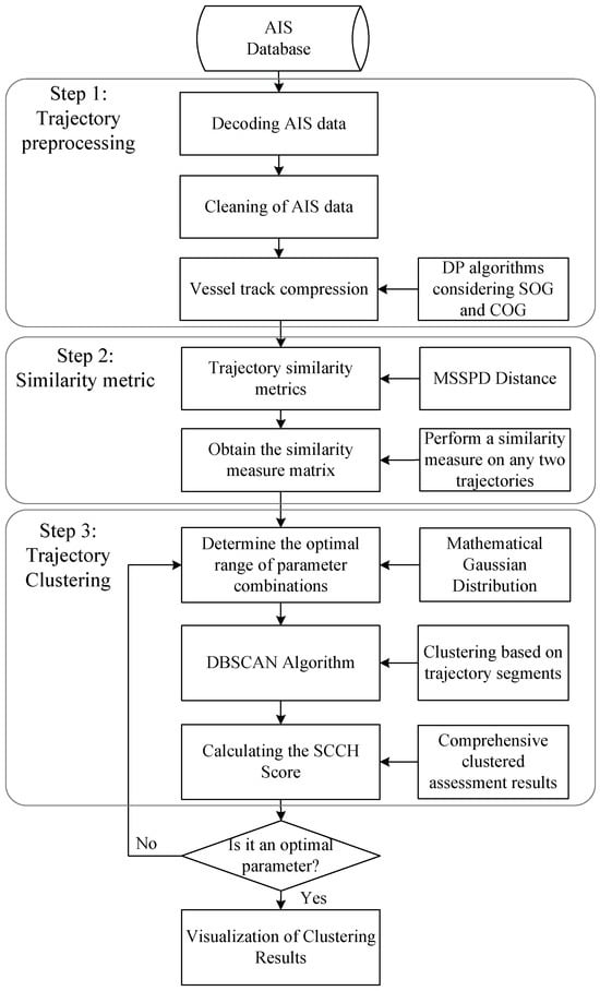
Figure 1.
Algorithm flow chart.
2.1. Trajectory Compression
2.1.1. Improve the Theory of the DP Algorithm
First proposed by David Douglas and Thomas Peucker in 1973, this algorithm is a classic line element-simplifying algorithm [23]. To process many redundant geometric data points, the DP algorithm is mainly used. While compressing the trajectory, this algorithm can preserve the shape characteristics of the trajectory. Nevertheless, the traditional algorithm solely considers the shape attributes of the trajectory. In this regard, an improved DP algorithm is proposed, which fully considers the spatial characteristics and the motion characteristics of the ship motion. The theoretical algorithm is shown in Figure 2.
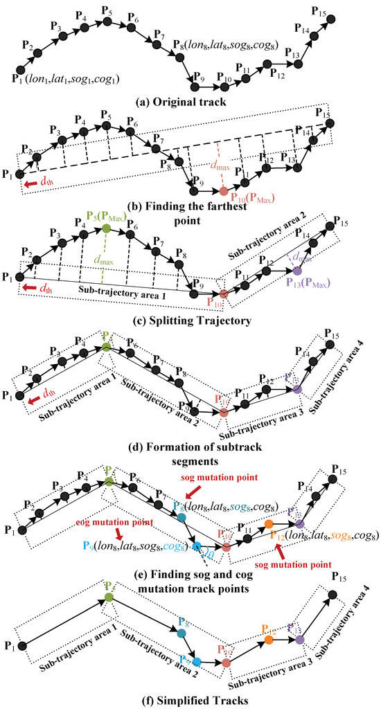
Figure 2.
Theoretical Schematic of the Improved DP Algorithm.
The trajectories of all ships within the studied area can be denoted as , with indicating the ship ’s trajectory and representing the total number of ships. The trajectory of the ship is defined as , where is the sequence index number of the length of the ship’s trajectory, is the total length of the ship’s trajectory, is the state vector of the ship at trajectory point , and are the position information of the ship at , is the ship’s speed to the ground at , and is the ship’s heading to ground at . The specific algorithm steps are as follows:
Step 1. Connect the first trajectory point () and the last trajectory point () to obtain a straight line; calculate the distance from all intermediate trajectory points to the line and obtain the maximum value , as shown in Figure 2b.
Step 2. Compare the distance with the predefined segmentation threshold . If , go directly to Step 4; if , keep the point corresponding to , which is noted as the segmentation point, and divide the original trajectory into two parts according to this segmentation point, as shown in Figure 2c.
Step 3. Repeat Step 2 until the trajectory cannot be cut, as shown in Figure 2d.
Step 4. Form the sub-trajectory area according to the split trajectory point. Calculate the steering angle ( = ) and ( = ); traverse the sub-trajectory region, compare with the speed threshold and with in turn; if , keep the trajectory point and record as the SOG mutation point; if , compare with the steering angle threshold ; if , keep the trajectory point and record as the speed mutation point; if , proceed to judge the next trajectory point, as shown in Figure 2e.
Step 5. Execute Step 4 recursively until all sub-trajectories have been traversed.
Step 6. Retain the final segmented trajectory points, the SOG mutation points, and the COG mutation points, as shown in Figure 2f.
2.1.2. Compression Threshold Determination
For the threshold value of the improved DP algorithm, not only the segmentation threshold but also the velocity threshold and the steering angle threshold should be determined. If the threshold value is too small, the accuracy of the segmented trajectory points will be higher but the algorithm overhead time will also be higher. If the threshold is too large, the accuracy of the trajectory will be worse but the simplicity of the data will be ensured. For each attribute of the ship’s AIS data, the method of determining the threshold value one by one is used to balance accuracy and simplicity.
First, the segmentation threshold is determined, and the Maritime Mobile Service Identity (MMSI) code is 413376XXX as an example. The original trajectory of 413376XXX is 3769 data points, as shown in Figure 3a. The idea of the threshold being 0.8 times the length of the ship is referenced in our selection process [5]. Table 1 shows the number of trajectory divisions and compression rates when the threshold values are 10 m, 50 m, 100 m, 150 m, and 200 m, respectively. As shown in Table 1, high compression ratios can be achieved for small threshold values. For the threshold of 10 m, the trajectory compression ratio is 86.41%. As the threshold value increases, the compression ratios do not significantly increase. To preserve the original trajectory’s shape as much as possible during the compression, the trajectory segmentation threshold is set to 100 m, as shown in Figure 3b.
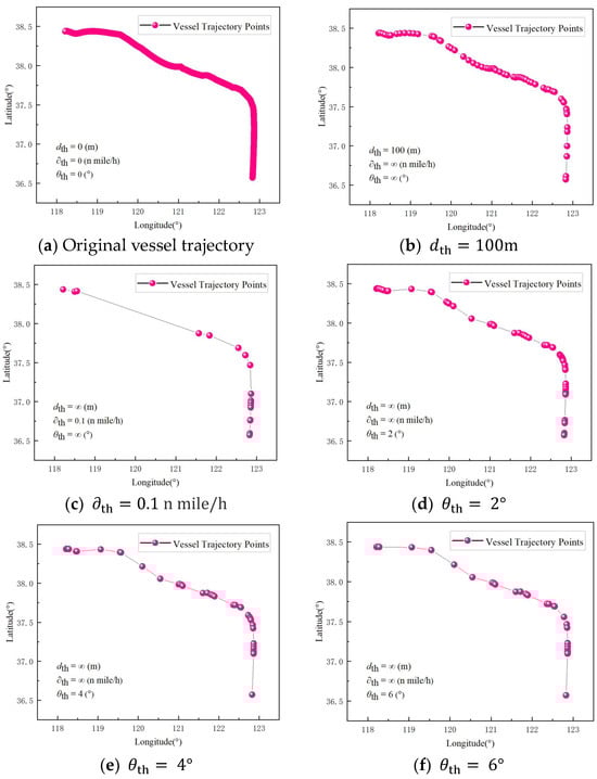
Figure 3.
Trajectory splitting graph under different thresholds.

Table 1.
The number of ship trajectories under different split thresholds.
After determining the segmentation threshold, we also need to determine the speed threshold and the steering angle threshold . We mainly cluster the moving trajectory of the ship, so we need to distinguish the ship’s grounding point and the ship’s moving point. In determining the speed threshold of the ship’s stranding point and the ship’s moving point, we find that the scattered points of the ship’s trajectory are mostly in the range of 0–1 knots for sailing speed, and there are no continuous trajectory points [24]. Therefore, 1 knot is chosen as the threshold value to distinguish the ship’s stranding points and moving points.
According to the ITU research result in ITU-R M.1371-5 Recommendation “Technical characteristics for an automatic identification system using time division multiple access in the VHF maritime mobile frequency band”, Appendix 1 (Operating characteristics of AIS using TDMA technology in the VHF maritime mobile frequency band), the reporting interval for ships underway is between 2 s and 10 s [25]. Considering the time delay of the approximated trajectory, 0.1 n mile/h is chosen as the selection. Figure 3c shows the trajectory division with without considering the segmentation threshold and the steering angle threshold . These retained trajectory points are the velocity mutation points.
Finally, to select the steering angle threshold , the method of first estimating the range of the threshold and then determining the final threshold from the experimental effect map is used. Based on the visual experience and the reporting interval of the ITU-R M.1371-5 proposal for changing course vessels [25], the range of is estimated to be 2–6° with the step size of 2°. When , as shown in Figure 3d, the compressed trajectory retains the heading information of the original ship trajectory to a large extent. In the data mining of the massive AIS data, the operation efficiency of the algorithm is considered, so it is not appropriate to choose as the steering angle threshold. When the steering angle threshold is , as shown in Figure 3e, the compressed trajectory generally retains the motion information of the original trajectory, but the local area is more coarsely represented. Figure 3f shows the compressed trajectory when . The compressed trajectory not only has overall simplicity but also has rich local heading information. Finally, is selected as the steering angle threshold for the improved DP algorithm.
After determining the thresholds for each attribute, we load the original trajectory and the compressed trajectory into the electronic chart for display, as shown in Figure 4. Since our algorithm is improved based on the DP algorithm, the compressed trajectory retains the shape of the original ship trajectory.
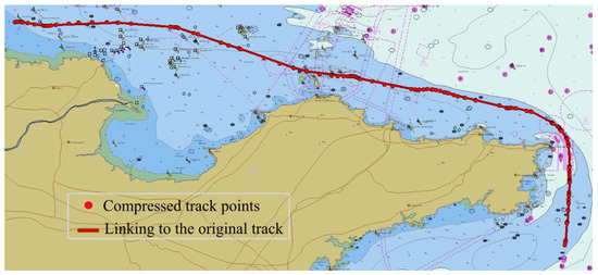
Figure 4.
View of vessel tracks from electronic charts.
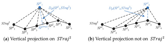
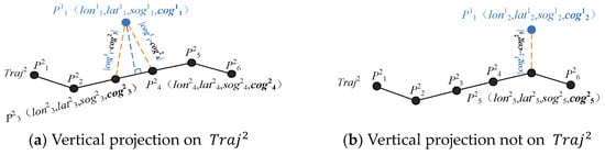
To demonstrate the advantages of our proposed algorithm, the 3D plots of the original trajectory and the 3D plots of the compressed trajectory are made based on the and the , respectively (see Figure 5). As shown in Figure 5a, the influences of weather, geography, and surrounding ships cause the variable speed of the ship during navigation.
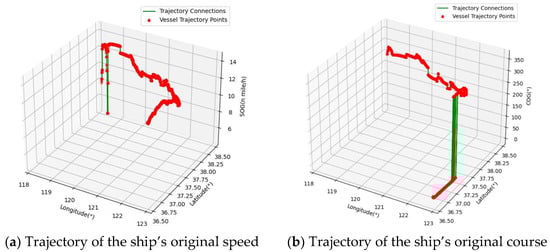
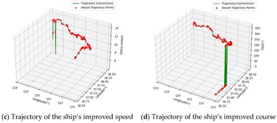
Figure 5.
Vessel 3D Trajectory Chart.
The complexity of the variation in heading exceeds that of speed. To provide a detailed representation of the COG compression, we intercept a portion of the raw AIS data that correlates with Figure 5. This interception is depicted in Table 2. Figure 5b and Table 2 demonstrate that the COG of some trajectory points displays either a step or continuous step change over a given period. As 0° and 360° share equivalence, the actual true heading changes remain minor. To preserve the original trajectory’s kinematic properties, the step changes are retained while compressing the COG. Mining, and thus clustering the ship’s AIS data, and the split target trajectory have two requirements: (1) Remove duplicate data and keep the trajectory concise to improve the efficiency of the algorithm. (2) Whether based on position or speed or heading, the mutation points of the trajectory are largely preserved to increase the similarity to the original trajectory. The final number of trajectories compressed by the algorithm is 239, and the compression rate is as high as 93.65%. Figure 5c, d show the 3D map of the trajectory after applying the improved DP algorithm. It can be seen from the figures that the compressed trajectory, corresponding to the original trajectory 3D map, retains the abrupt change points of the speed and the abrupt change points of the heading accordingly, which is most obvious around the cliff area.
Table 2.
Raw AIS data (MMSI:413376XXX).
2.2. Similarity Metric
2.2.1. SSPD
The SSPD is a shape-based distance proposed by Besse et al. in 2016 [12]. It is a shape similarity metric that uses the distance from a point to a line segment instead of the distance between points. Based on the following three reasons, we believe that the SSPD is the most appropriate method for measuring trajectory similarity. Firstly, the SSPD uses the average distance, and the algorithm is easy to understand and resistant to noise. Secondly, the SSPD uses the distance from the point to the line segment and solves the sampling rate problem. When trajectories are compressed, the distances between trajectories do not change significantly. Thirdly, although the SSPD is a shape similarity measure, it can be incorporated into other attributes of AIS data. Calculating distances in a multi-attribute sequence gives SSPD the ability to identify directions. The SSPD algorithm is defined as follows:
Definition 1.
(Trajectory string and location coordinates): From the previous section, the ship’s trajectory is defined as . is the state vector of the ship at trajectory point , and are the position information of the ship at .
Definition 2.
(Trajectory segment): In the trajectory , the segment of the trajectory where two points are connected is defined as , where .
Definition 3.
(Distance from trajectory point to trajectory): The main idea of the SSPD is to find the shortest distance between each trajectory point in the trajectory to the line segment connecting two adjacent trajectory points of another trajectory. As shown in Figure 6a, if the vertical projection is on , then the distance from to is . As shown in Figure 6b, if the vertical projection is not on , then the distance from to is .
Figure 6.
Distance between a point and a trajectory based on SSPD.
Definition 4.

(Asymmetric segmentation path distance): As shown in Figure 7a, the asymmetric segmentation path distance (SPD) from the trajectory to the trajectory is the average of the shortest distance from all points of the trajectory to the trajectory . is the SPD from to . The formula is defined as follows:
Figure 7.
SSPD diagram.
is the distance from the trajectory point in to the trajectory. The formula is defined as follows:
is the minimum distance from the point to the line connecting two adjacent trajectories in the trajectory. The formula is defined as follows:
Definition 5.
(Symmetric segmentation path distance): As shown in Figure 7b, the SSPD between and is the average of the two SPDs. The formula is defined as follows:
In the above description, the advantages and principles of the SSPD are highlighted. However, the conventional SSPD also encounters the following issues when measuring the similarity of ship trajectories:
- The direction of the ship trajectory cannot be identified. In particular, the incoming and outgoing ship trajectories of the same channel may be divided into a cluster of trajectories due to the similarity of the SSPD.
- Low utilization of the ship navigation information. The COG and SOG are also important components of the ship navigation at sea. However, according to the above, the trajectory similarity metric using the traditional SSPD only considers the latitude and longitude.
2.2.2. MSSPD
To solve the above problem, we improve the traditional SSPD and propose the multi-attribute symmetric segmented path distance (MSSPD). The MSSPD integrates position information, velocity information, and heading information. The relevant definitions are as follows:
Definition 6.
(Trajectory string): From Section 2.2.1, the ship’s trajectory is defined as , where is the ship’s speed to ground at , and is the ship’s heading to ground at .
Definition 7.
(SOG distance between trajectories): Sailing speed varies for different types of ships. For example, the speed of ordinary cargo ships is 12–15 kn, and that of large container ships is 20–28 kn. Sailing speed is also affected by various factors such as wind and waves, current, cargo, etc. The speed of the same ship also changes constantly as it sails. We want to group the same type of ship trajectories into a cluster, so when studying the SOG distance between the ships, we use the difference between the mean values of two ship speeds to represent the SOG distance between two ship trajectories.
Definition 8.
(COG distance from trajectory point to trajectory): The calculation of the COG distance from the trajectory point to the trajectory is based on the premise of the SPD from the point to the trajectory. As shown in Figure 8a, the vertical projection of falls on the line segment . Calculate and and take the smaller value as the COG distance from the trajectory point to the trajectory . As shown in Figure 8b, the vertical projection of does not fall onto the trajectory , so is used as the COG distance from the point to the trajectory . The specific formula is as follows:
where denotes the COG distance from the trajectory point to the trajectory and denotes the COG distance from the point to the trajectory segment .
Figure 8.
COG distance from the point to the trajectory.
Definition 9.
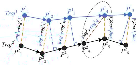
(COG distance from trajectory to trajectory): Considering two trajectories with different numbers of points, the symmetric COG distance (SCOG) based on trajectory to trajectory is proposed, as shown in Figure 9. The specific definition equation is as follows:
Figure 9.
COG distance from the trajectory to the trajectory.
is the one-way COG distance from the trajectory to the trajectory in Equation (9).
Definition 10.
(MSSPD): Now, we obtain the position-based metric distance SSPD, the speed-based SOG distance, and the heading-based COG distance. Based on the above analysis process, the MSSPD formula is formally given by:
where , , and are the weights of the three distances, .
2.2.3. Comparing Different Distances
An excellent trajectory distance can both accurately calculate the similarity between two trajectories and resist noise. To test the effectiveness of MSSPD, we design three sets of experiments. The first set of experiments is called compression experiments. The second set of experiments is called noise experiments. The third set of experiments is called direction experiments. In the three sets of experiments, we selected the commonly used ship inter-trajectory metric distances, which are the Fréchet, the Hausdorff, and the SSPD.
Three real ship trajectories in Chengshanjiao waters are selected, as shown in Figure 10. We can see that and are traveling from north to south, which are recorded as the outbound trajectories; is traveling from south to north, which is recorded as the inbound trajectory. To facilitate the observation of the change in the similarity metric distance of each trajectory, the method proposed by Zhang and Shi (2021) is cited [26]. is the distance change rate, , is the distance before the change, is the distance after the change, the name can be Fréchet, Hausdorff, SSPD, or MSSPD. Specific details of the three sets of experiments are given below:
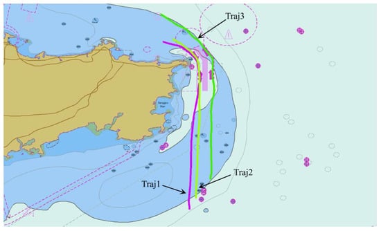
Figure 10.
Three original trajectories.
- Compression experiment. This experiment is used to test whether the distance of the trajectory similarity metric is affected by the compression algorithm. In this experiment, and are selected, where the original trajectory of is maintained and the trajectory is compressed using the proposed improved DP algorithm. The change in of each type of distance with the compression rate is observed.
- Noise experiment. This experiment is used to test whether the trajectory similarity metric distance is affected by noise. The algorithm selects and , leaves the original trajectory of unchanged, and artificially adds noise to . Observe the change in as the noise is gradually increased.
- Direction experiment. This experiment is used to test whether the trajectory similarity metric distance can detect two trajectories in opposite directions. The trajectories , , and are selected, and are calculated, and the values of the trajectory distances are observed.
Figure 11a shows the variation of with the compression rate, the Fréchet and the Hausdorff overlap in Figure 11a. The Fréchet and the Hausdorff have the most pronounced variation, indicating that the Fréchet and the Hausdorff are susceptible to the influence of the compression algorithm. The SSPD varies relatively smoothly, and the compression algorithm has less influence on the SSPD. For the MSSPD, a small compression rate corresponds to a low . As the compression rate gradually increases, the rate of change in the distance of the MSSPD also increases, accompanied by oscillations in the interior of the interval in between. The choice of different thresholds affects the compression performance of the MSSPD, and a reasonable threshold can avoid the influence of the compression algorithm on . This also indirectly illustrates the importance of Section 2.1.2.
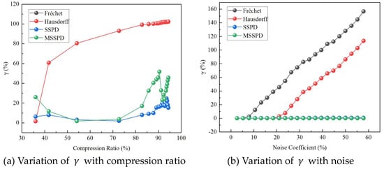
Figure 11.
Compression experiment and noise experiment.
Figure 11b shows the variation of with noise. The Fréchet and the Hausdorff are sensitive to noise points; the SSPD and the MSSPD are not. The reason is that the Fréchet and the Hausdorff use local distances instead of global distances. The SSPD and the MSSPD use the average distance for their metrics, and a small number of noise points have little effect overall.
Table 3 shows the distances between tracks for the same heading ( and ) and different headings ( and ) for the same channel. The Hausdorff and the SSPD have the least variation, and it would be difficult to distinguish tracks in opposite directions if they are mixed with tracks with large distances in the same heading. The Fréchet comes next, with discrimination between tracks in the opposite direction since the Fréchet calculates the distance in the time series. The MSSPD shows excellent direction discrimination and is sensitive to ship trajectories under different headings.
Table 3.
Nautical mile distance between tracks.
Through the above three experiments, three conclusions can be made when using MSSPD for the similarity metric of the trajectory clustering: First, if a suitable compression threshold is chosen, the results of the ship trajectory metric after the compression algorithm will not change. Second, a certain amount of noise does not affect the effect of the ship trajectory clustering. Finally, trajectories in opposite directions are distinguished.
2.3. Theory of the DBSCAN Algorithm
The DBSCAN algorithm is a data-clustering algorithm proposed in 1996 [27]. The DBSCAN algorithm uses two parameters to cluster line segments: and , where is the density radius and is the density threshold (see Figure 12). Lines are categorized as cores, densely connected lines, and anomalies. through represents the direct density, through represents the accessible density, and and represent the connected density, as shown in Figure 12b. According to these parameters, lines with similar densities are grouped into clusters. As shown in Figure 12c, if the neighborhood of sample contains less than but is in the neighborhood of other kernel points, then the sample point is said to be the sample boundary. And all lines that have no density connection with other lines are outliers, i.e., noise, as shown in Figure 12d.
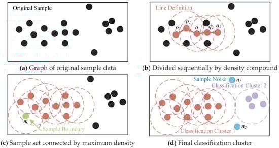
Figure 12.
Schematic of the DBSCAN algorithm.
The principle of DBSCAN is to detect all line segments connected to the density and group them into a cluster of trajectories. The problem with the DBSCAN algorithm is the choice of parameters and . One configuration may place each trajectory in a large cluster, while another configuration may not identify any clusters and designate each trajectory as noise.
2.4. SCCH Score
To evaluate the excellence of the algorithm and adaptively select the optimal parameters of the DBSCAN algorithm, a comprehensive index for clustering performance, the SCCH, is proposed. Considering the validity and reliability of the algorithm, the proposed clustering performance index integrates the CH score and the SC score, and the SCCH score is defined as:
where and denote the SC score and CH score of the clustering results obtained for the current input parameters, respectively. and denote the SC score vector and the CH score vector of the clustering results obtained for all input parameters, respectively. and are the normalized results of the SC score and the CH score. The larger the , the better the clustering effect.
3. Case Study
3.1. Data Characterization and Vessel Track Compression
The aim of the ship trajectory clustering is to group trajectories that have high density and similar headings into one class, maximizing the distribution density. Each trajectory cluster should have a fixed number of trajectories, and the maximum distribution density should be ensured. Because the trajectory heading is approximately consistent within each cluster, we can derive the customary paths of ships in each cluster. Subsequently, we can extract the customary shipping paths and the traffic flow-related data for all ships in the study area.
Vessel trajectory clustering is an important instrument for studying vessel behavior patterns, which can provide a reference frame for vessel behavior detection and traffic pattern recognition. In this paper, the AIS data obtained from the Bohai Sea waters are used to extract the regular routes of ships in the Bohai Bay waters using DBSCAN clustering based on the similarity metric distance of the MSSPD. The AIS data (such as ship maritime identification code, latitude, longitude, speed, course to ground, and heading) of the sea area in Bohai Bay from 1 to 3 May 2019 are selected. A total of 207,878 original ship track data from 203 ships in the sea area are obtained. Data cleaning and data restoration are performed on the original AIS data; finally, the restored AIS data are compressed using the proposed improved DP algorithm. The number of vessels and the number of trajectory points for each algorithm are shown in Table 4. As shown in Figure 13, the direction and shape of the ship trajectory do not change after compression, and the computational efficiency is significantly improved, which lays a solid foundation for the subsequent similarity measurement. Based on this, it is possible to conduct data mining on ship features, cluster trajectories, and detect anomalies in ship trajectories.
Table 4.
Number of ships and track points after different algorithms.
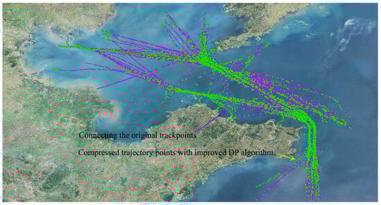
Figure 13.
Vessel trajectory map with improved DP algorithm.
3.2. Trajectory Clustering
The compressed finished AIS data were experimented on with the DBSCAN clustering based on the MSSPD algorithm. Through extensive analysis and experimental comparisons, , , and are set to [0.6, 0.2, 0.2]. The DBSCAN algorithm has two input parameters that must be manually determined, and . Different combinations of these parameters have a significant impact on the final clustering results. In our experiments, the parameter determination consists of two steps. The first step is to compute all parameter combinations based on the statistical relationship between the two parameters, which transforms the problem of determining the two parameters into the problem of selecting the parameter combinations. The second step is to select specific parameter combinations based on the SCCH score. In the first step, we use the method proposed by Zhao and Shi (2019) [10]. This study states that for fixed , the core distance value that allows the most line data to be the core line is the appropriate parameter . Based on the values of all the line data, the inverse Gaussian distribution is used to determine the appropriate parameter . Therefore, we obtain all the parameter combinations according to the above method. In the second step, we select the best parameter combination based on the SCCH score. Finally, we set the number of from 2 to 5 and the range of values from 0.015 to 0.065. Table 5 shows the score values after each parameter change.
Table 5.
SCCH scores for the MSSPD-based DBSCAN algorithm.
As shown in Table 5, when and , and the highest scores of and are achieved simultaneously. These parameters are input into the DBSCAN algorithm, and the clustering results of ship trajectories are shown in Figure 14. To emphasize the visual impact of the final clustering, we display it on the global and detail maps, respectively. As the DBSCAN identifies noise, the global maps feature trajectory maps that include and exclude noise (see Figure 14a,b), whereas the detail maps show the traffic distribution in the Laotieshan, Penglai, and Chengshanjiao waters (see Figure 14c–e).
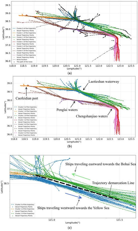
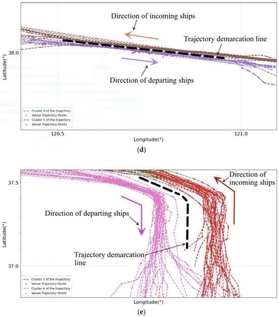
Figure 14.
The clustering results of ship trajectories; (a) Map of global trajectories with noise; (b) Map of global trajectories after removal of noise; (c) Detailed view of the Laotieshan waterway; (d) Detailed view of the Penglai waters; (e) Detailed view of the Chengshanjiao waters.
The global map shows that some noise trajectories cross between different sea areas, and others are reflected in the drift of short trajectories. Individual trajectory clusters are well organized and there is no visual fragmentation. Two things are discernible from the detailed drawings. First, the detailed drawings can identify the primary shipping lanes in a particular water body. Secondly, different vessel paths when traveling in opposite directions are distinguished with ease. In the following sections, the extracted clusters of trajectories will be analyzed and discussed in more detail.
3.3. Distribution of Extracted Traffic
After analyzing and summarizing the clustering results, we successfully extract seven groups of track clusters in the Bohai Sea area, as shown in Figure 15. By analyzing the extraction results of the Bohai Sea waters, we can find that our method has the following characteristics:
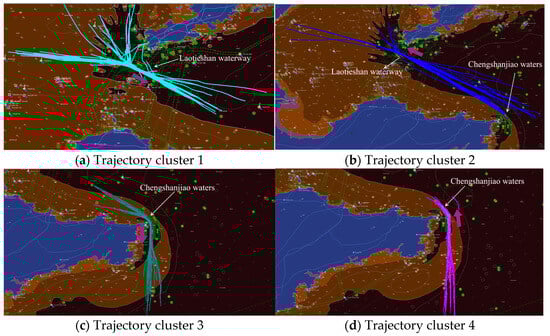
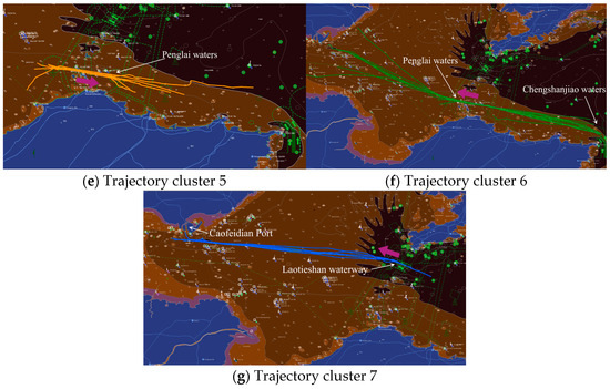
Figure 15.
Final 7 trajectory cluster groups (The red arrow in the figure represents the direction of navigation).
- Extraction of shipping routes in different waters. Figure 15a,b,g show the ship traffic flow in Laotian waters. Figure 15c,d show the vessel traffic flow in Chengshanjiao waters. Figure 15e,f show the traffic flow in Penglai waters. The noise is filtered out, leaving the traffic conditions of each water separately, which in turn can be analyzed for the traffic of specific waters.
- Extraction of different shipping routes in the same waters. In Laotieshan waterway, Figure 15a,b extract the traffic routes to and from Chengshanjiao waterway and Laotieshan waterway, while Figure 15g extracts the traffic flow from Laotieshan waterway to Caofeidian port. By extracting different routes in the same water area, navigation patterns on various routes can be identified. This could provide a more objective basis for decision making by maritime traffic safety management.
- Identification of trajectory direction, taking Laotieshan waterway as an example for illustration. The Laotieshan Channel is a significant passage for large ships traveling to and from the Bohai Sea. Most ships travel between the west of the Bohai Sea and the east of the Yellow Sea through the Laotieshan Channel. The red arrow in the figure represents the direction of navigation. The westbound ship traffic is located on the barrier’s north side in the Laotieshan waterway, as shown in Figure 15b. Figure 15a shows that the eastbound ship traffic flow is located on the south side of the Laotieshan waterway barrier. The ability to detect the trajectory direction is due to the introduction of the MSSPD, which makes our method more efficient.
4. Discussion
4.1. Comparison with Other Clustering Algorithms
In the previous section, we investigated the trajectory clustering process of the MSSPD-based DBSCAN arithmetic in the Bohai Sea area through the specific case study. This section compares and discusses the algorithm to the SSPD-based DBSCAN clustering and the MSSPD-based spectral clustering. The method based on SSCH scores is still used for selecting parameters for the comparison algorithm.
4.1.1. DBSCAN Algorithm Based on SSPD
We select the same AIS data for the comparison experiments. First, experiments are conducted with the DBSCAN algorithm based on the SSPD. The results of the DBSCAN algorithm are given in Table 6, and we finally choose and as the inputs to the above algorithm. Figure 16 shows the final clustering results of the DBSCAN algorithm based on the SSPD after filtering out the noise.
Table 6.
SCCH scores for the SSPD-based DBSCAN algorithm.
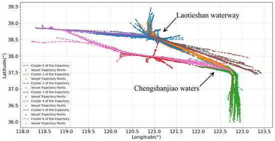
Figure 16.
DBSCAN algorithm based on SSPD.
Different colors in the figure represent different classification clusters. We mainly analyze the Laotieshan waters and Chengshanjiao waters.
- In the Laotieshan waters, the intersection of each cluster is slightly patchy, but the individual channels in the waters are extracted. This is since the SSPD is a metric based on the average distance between track points and track segments, and the SSPD is highly discriminative between tracks with different destinations in the same waters. It is also noise resistant. These properties are superior to the Hausdorff distance.
- In Chengshanjiao waters, the clustering effect is not optimistic. In the previous section, we analyzed two routes in Chengshanjiao waters; one was the incoming trajectory and the other was the outgoing trajectory. In the DBSCAN algorithm based on the SSPD, it appears that the inbound and outbound trajectories are grouped into one class. This is since the traditional SSPD is only the similarity measure for the ship’s position and does not consider the multidimensional information of the AIS data.
4.1.2. Spectral Clustering Algorithm Based on MSSPD
Finally, we use spectral clustering to mine ship trajectories. The similarity metric between trajectories uses our proposed the MSSPD. The spectral clustering is an algorithm developed from graph theory that uses the principle of tangent graphs to partition clusters. The spectral clustering is also sensitive to the choice of parameters. Figure 17 demonstrates the trends of various metric scores of the spectral clustering concerning the -value of the categorized clusters.
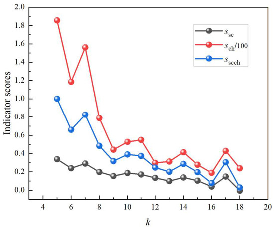
Figure 17.
Indicator scores for each category based on spectral clustering.
As the -value increases, the scores of each category generally show a decreasing trend but are accompanied by oscillations. After the first oscillation, a steep spike occurs at , when the SCCH has the highest score after the initial value. To avoid the local optimality, experiments for and are performed in turn. Figure 18a and 18b correspond to the final results of the spectral clustering at and respectively. In Figure 18a, the green clusters of trajectories pass through the Laotieshan waterway and the Penglai waters, respectively, but are grouped into the same cluster in the area near Caofeidian Port. In addition, although the spectral clustering can spatially cluster samples of arbitrary shape, it cannot detect noise. Figure 18c shows a detailed view of the Laotieshan waterway. The clusters of different types of traces in the figure are always interspersed with each other, which is visually reflected in the highly mottled colors.
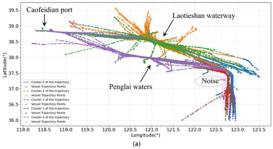
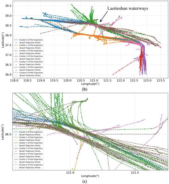
Figure 18.
Spectral clustering based on MSSPD; (a) Spectral clustering at ; (b) Spectral clustering at ; (c) Detailed view of the Laotieshan waterway.
5. Conclusions
In this paper, we present the MSSPD and a new approach to consider SOG and COG when analyzing AIS trajectory data. Vessel trajectories are compressed using the enhanced DP algorithm. The MSSPD is chosen as the similarity metric between the trajectories. The DBSCAN algorithm is used to cluster ship trajectories in the Bohai Sea area. The adaptive selection of the parameters of the DBSCAN algorithm is realized by using the SCCH index. The conclusions of this study are as follows.
- The SOG and COG are considered to improve the DP algorithm. Position compression, velocity compression, and heading compression of trajectories are realized. The compression thresholds of each attribute are established one by one. When setting the compression thresholds at , , and , a balance of the conciseness and reliability can be achieved, which is a prerequisite for the accurate MSSPD metrics.
- For the multidimensional information of AIS data, the MSSPD is proposed and compression, noise, and directional experiments are conducted, respectively. For compression resistance, adjusting the appropriate compression threshold can effectively reduce the impact of the compression algorithm on the MSSPD and decrease to below 20%. With regard to the average distance used by the MSSPD, as the noise coefficient increases, remains stable with an amplitude ranging between 0% and 2%. In Section 2.2.3, and , which indicates that the MSSPD is sensitive to the trajectory’s direction. The MSSPD achieves better results in all three evaluation indices.
- For the problem of selecting clustering parameters, we propose the SCCH evaluation index. By analyzing the SCCH scores, we found that the SCCH achieves the highest score when is set to 0.05 and to 5. The SCCH score is utilized for adaptive parameter selection, and the algorithmic process is automated without requiring human intervention. Through experimental comparisons, we believe that the clustering algorithm that combines well with the MSSPD is the DBSCAN. Whether extracting different routes in the same water or extracting shipping lanes in different waters, the DBSCAN based on the MSSPD provides excellent performance.
However, our proposed method is not a generalized case solver and should be further estimated on all types of AIS data to verify its repeatability and reliability. The threshold selection of the compression algorithm needs to be more flexible and precise. Also, the selection of the MSSPD weights needs to be rationalized according to the AIS data from different sea areas. This will also be one of the future research directions.
Author Contributions
C.L.: Conceptualization, Methodology, Project management. S.Z.: Design, Methodology, Algorithm, Software. L.C.: Validation, Software. B.L.: Data curation. All authors have read and agreed to the published version of the manuscript.
Funding
The work was supported by the National Key Research and Development Program of China (No. 2019YFE0111600), National Natural Science Foundation of China (No. 61971083, No. 51939001, and No. 62371085), LiaoNing Revitalization Talents Program (No. XLYC2002078) and Fundamental Research Funds for the Central Universities (No. 3132023514).
Institutional Review Board Statement
Not applicable.
Informed Consent Statement
Not applicable.
Data Availability Statement
Data available on request due to restrictions of privacy.
Conflicts of Interest
The authors declare no conflict of interest.
References
- IMO. SOLAS Consolidated Edition; IMO: London, UK, 2014; ISBN 978-92-801-1549. [Google Scholar]
- Mazaheri, A.; Montewka, J.; Kujala, P. Towards an evidence-based probabilistic risk model for ship-grounding accidents. Saf. Sci. 2016, 86, 195–210. [Google Scholar] [CrossRef]
- Gil, M.; Montewka, J.; Krata, P.; Hinz, T.; Hirdaris, S. Determination of the dynamic critical maneuvering area in an encounter between two vessels: Operation with negligible environmental disruption. Ocean Eng. 2020, 213, 107709. [Google Scholar] [CrossRef]
- Li, Y.; Liu, R.W.; Liu, J.; Huang, Y.; Hu, B.; Wang, K. Trajectory compression-guided visualization of spatio-temporal AIS vessel density. In Proceedings of the 2016 8th International Conference on Wireless Communications & Signal Processing, Yangzhou, China, 13–15 October 2016; pp. 1–5. [Google Scholar]
- Zhang, S.; Liu, Z.; Cai, Y.; Wu, Z. Shi GAIS trajectories simplification threshold determination. J. Navig. 2016, 69, 729–744. [Google Scholar] [CrossRef]
- Zhao, L.; Shi, G. A method for simplifying ship trajectory based on improved Douglas–Peucker algorithm. Ocean Eng. 2018, 166, 37–46. [Google Scholar] [CrossRef]
- Patroumpas, K.; Alevizos, E.; Artikis, A.; Vodas, M.; Pelekis, N.; Theodoridis, Y. Online event recognition from moving vessel trajectories. GeoInformatica 2017, 21, 389–427. [Google Scholar] [CrossRef]
- Wang, L.; Chen, P.; Chen, L.; Mou, J. Ship AIS Trajectory Clustering: An HDBSCAN-Based Approach. J. Mar. Sci. Eng. 2021, 9, 566. [Google Scholar] [CrossRef]
- Zhang, M.; Kujala, P.; Musharraf, M.; Zhang, J.; Hirdaris, S. A machine learning method for the prediction of ship motion trajectories in real operational conditions. Ocean Eng. 2023, 233, 114905. [Google Scholar] [CrossRef]
- Zhao, L.; Shi, G. A trajectory clustering method based on Douglas-Peucker compression and density for marine traffic pattern recognition. Ocean Eng. 2019, 172, 456–467. [Google Scholar] [CrossRef]
- Buchin, K.; Buchin, M.; Wang, Y. Exact Algorithms for Partial Curve Matching via the Fréchet Distance. In Proceedings of the Twentieth Annual ACM-SIAM Symposium on Discrete Algorithms, SODA 2009, New York, NY, USA, 4–6 January 2009; ACM: New York, NY, USA, 2009. [Google Scholar] [CrossRef]
- Besse, P.; Guillouet, B.; Loubes, J.M.; François, R. Review and Perspective for Distance Based Trajectory Clustering. Comput. Sci. 2015, 47, 169–179. [Google Scholar] [CrossRef][Green Version]
- Wei, Y.; Chen, Z.; Zhao, C.; Chen, X.; He, J.; Zhang, C. A time-varying ensemble model for ship motion prediction based on feature selection and clustering methods. Ocean Eng. 2023, 270, 113659. [Google Scholar] [CrossRef]
- Xu, X.; Liu, C.; Li, J.; Miao, Y.; Zhao, L. Long-Term Trajectory Prediction for Oil Tankers via Grid-Based Clustering. J. Mar. Sci. Eng. 2023, 11, 1211. [Google Scholar] [CrossRef]
- Mou, J.M.; Chen, P.F.; He, Y.; Zhang, X. Fast adaptive spectral clustering algorithm for ship AIS trajectory. J. Harbin Eng. Univ. 2018, 39, 428–432. [Google Scholar]
- Gao, M.; Shi, G.Y. Ship-handling behavior pattern recognition using AIS sub-trajectory clustering analysis based on the T-SNE and spectral clustering algorithms. Ocean Eng. 2020, 205, 106919. [Google Scholar] [CrossRef]
- Cao, Y.Y.; Cui, Z.M.; Wu, J. A vehicle trajectory pattern learning method with improved Hausdorff distance and spectral clustering. Comput. Appl. Softw. 2012, 29, 38–40+113. [Google Scholar]
- Yang, C.H.; Lin, G.C.; Wu, C.H.; Liu, Y.-H.; Wang, Y.-C.; Chen, K.-C. Deep Learning for Vessel Trajectory Prediction Using Clustered AIS Data. Mathematics 2022, 10, 2936. [Google Scholar] [CrossRef]
- Xu, X.; Liu, C.; Li, J.; Miao, Y. Trajectory clustering for SVR-based Time of Arrival estimation. Ocean Eng. 2022, 259, 111930. [Google Scholar] [CrossRef]
- Wu, W.; Chen, P.; Chen, L.; Mou, J. Ship Trajectory Prediction: An Integrated Approach Using ConvLSTM-Based Sequence-to-Sequence Model. J. Mar. Sci. Eng. 2023, 11, 1484. [Google Scholar] [CrossRef]
- Yang, J.; Liu, Y.; Ma, L.; Ji, C. Maritime traffic flow clustering analysis by density-based trajectory clustering with noise. Ocean Eng. 2022, 249, 236–249. [Google Scholar] [CrossRef]
- Guo, S.Q.; Mou, J.M.; Chen, L.; Chen, P. Improved kinematic interpolation for AIS trajectory reconstruction. Ocean Eng. 2021, 234, 245–257. [Google Scholar] [CrossRef]
- Douglas, D.H.; Peucker, T.K. Algorithms for the reduction of the number of points required to represent a digitized line or its caricature. Cartogr. Int. J. Geogr. Inf. Geovisualization 1973, 10, 112–122. [Google Scholar] [CrossRef]
- Xu, X.F.; Cui, D.Q.; Li, Y.; Xiao, Y. Research on Ship Trajectory Extraction Based on Multi-Attribute DBSCAN Optimisation Algorithm. Pol. Marit. Res. 2021, 28, 136–148. [Google Scholar] [CrossRef]
- Series, M. Technical Characteristics for an Automatic Identification System Using Time-Division Multiple Access in the VHF Maritime Mobile Band; Recommendation ITU: Geneva, Switzerland, 2014; pp. 1371–1375. [Google Scholar]
- Zhang, Y.Q.; Shi, G.Y. Trajectory Similarity Measure Design for Ship Trajectory Clustering. In Proceedings of the 2021 IEEE 6th International Conference on Big Data Analytics (ICBDA), Xiamen, China, 5–8 March 2021; IEEE: Piscataway, NJ, USA, 2021. [Google Scholar] [CrossRef]
- Ester, M.; Kriegel, H.P.; Sander, J.; Xu, X. A Density-Based Algorithm for Discovering Clusters in Large Spatial Databases with Noise; AAAI Press: Menlo Park, CA, USA, 1996. [Google Scholar]
Disclaimer/Publisher’s Note: The statements, opinions and data contained in all publications are solely those of the individual author(s) and contributor(s) and not of MDPI and/or the editor(s). MDPI and/or the editor(s) disclaim responsibility for any injury to people or property resulting from any ideas, methods, instructions or products referred to in the content. |
© 2023 by the authors. Licensee MDPI, Basel, Switzerland. This article is an open access article distributed under the terms and conditions of the Creative Commons Attribution (CC BY) license (https://creativecommons.org/licenses/by/4.0/).