
Dynamic Multi-Period Maritime Accident Susceptibility Assessment Based on AIS Data and Random Forest Model

 ,
,
Abstract
:1. Introduction
2. Materials
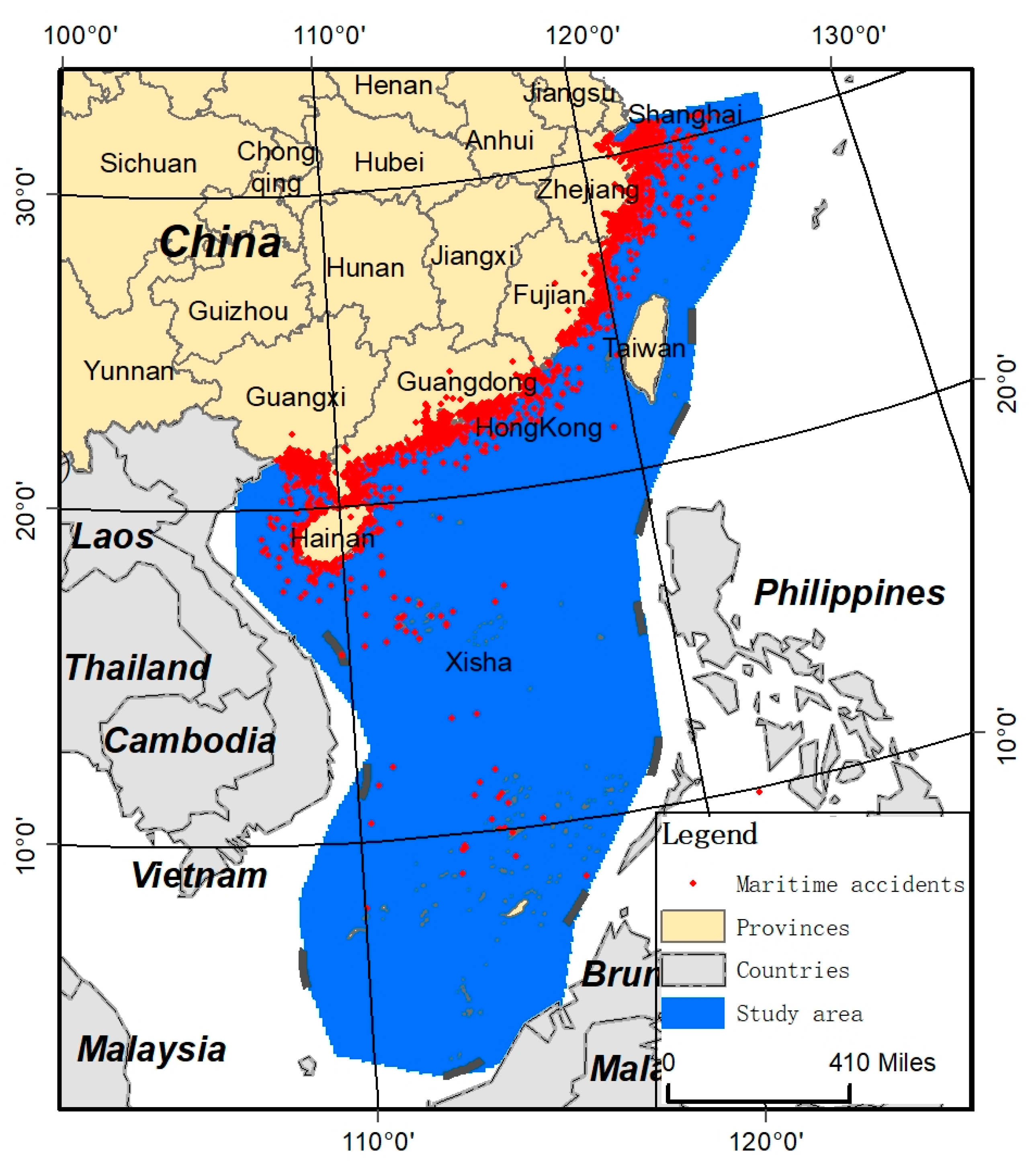
2.1. Study Area
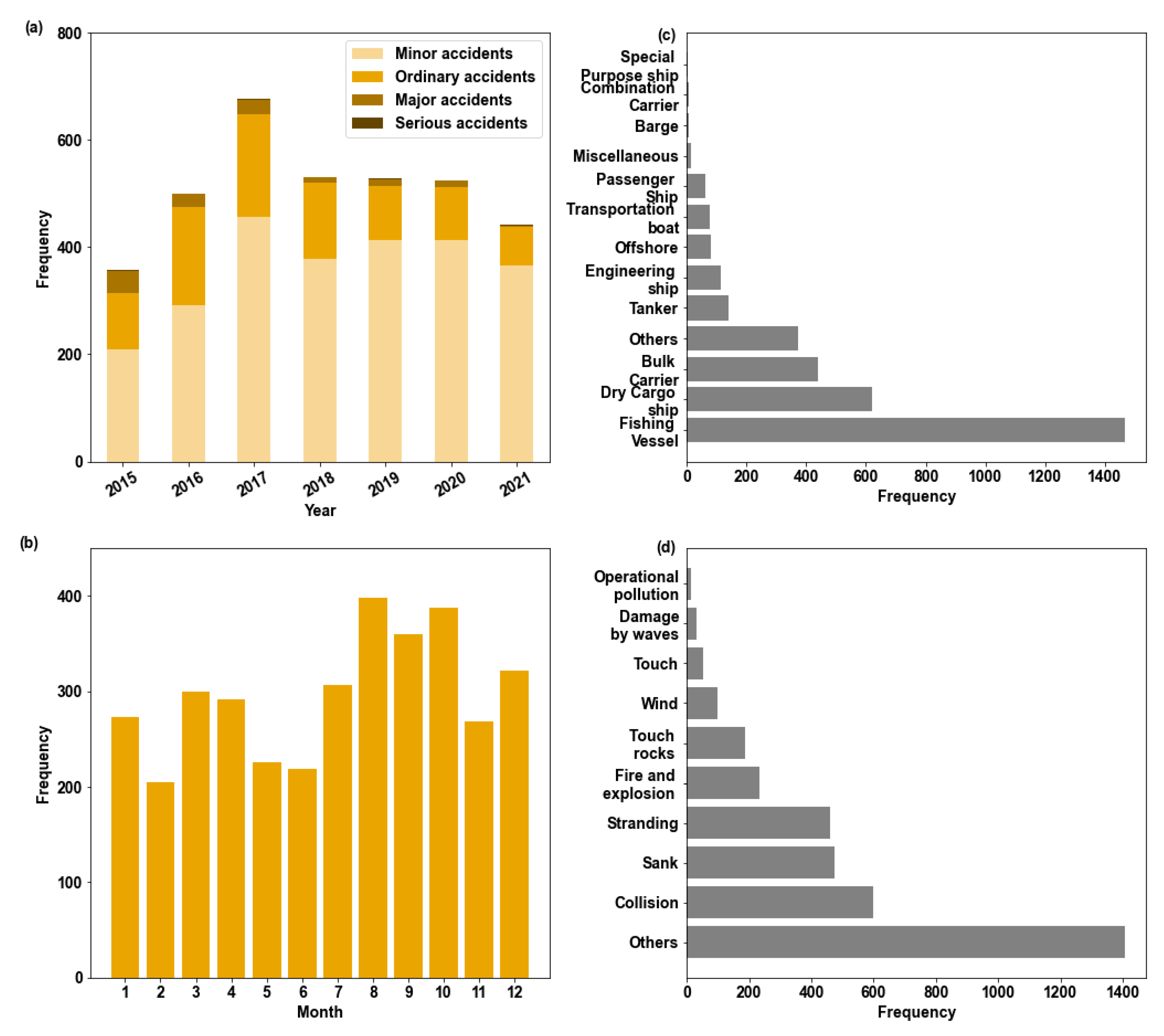
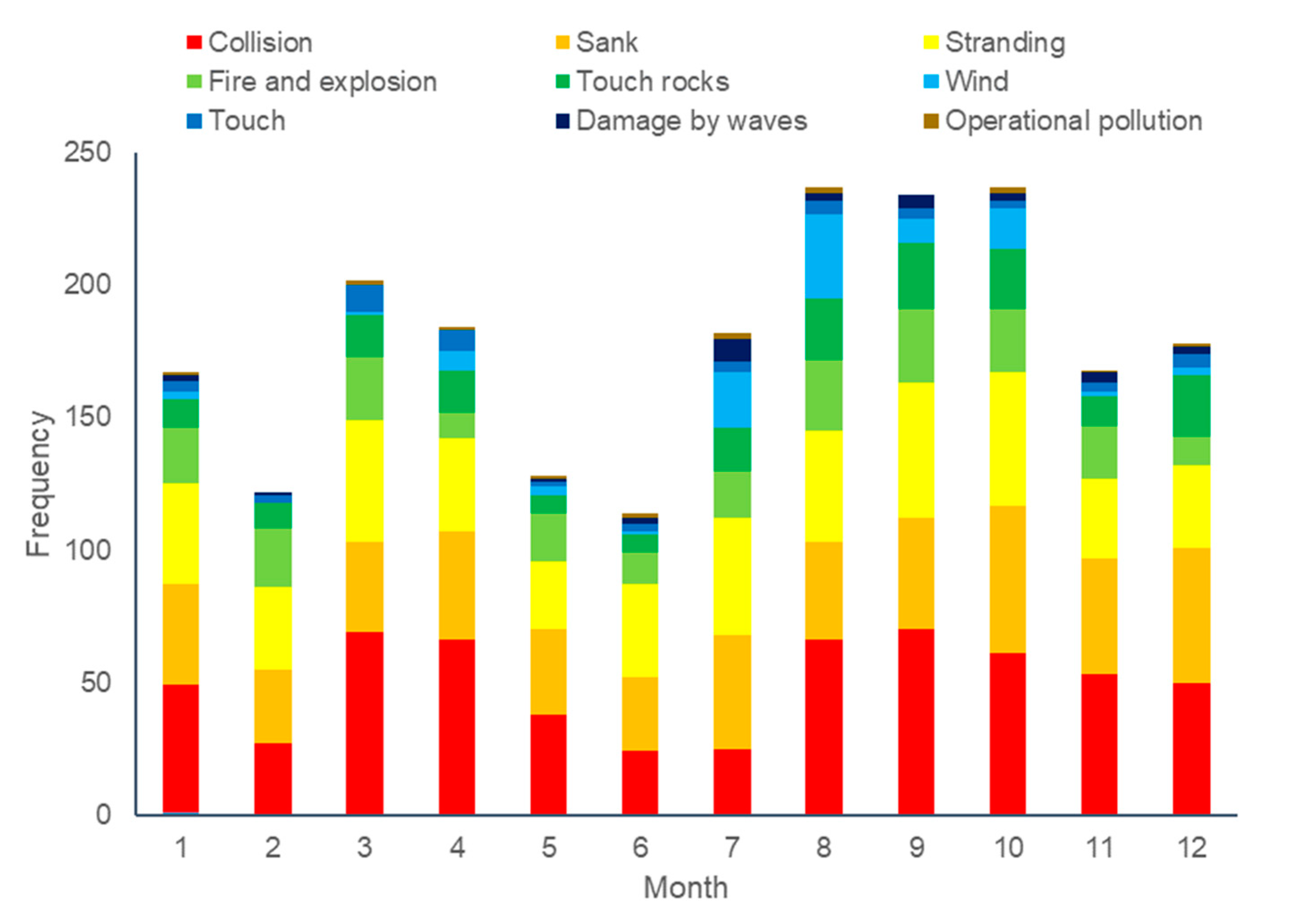
2.2. Maritime Accident Data
2.3. Accident-Influencing Factors
2.3.1. Ship Features
2.3.2. Static Environmental Features
2.3.3. Dynamic Weather Features
3. Methodology
3.1. Random Forest Model
3.2. Generation of Feature Matrixes
3.3. Feature Selection
3.4. Construction of Training and Testing Datasets
3.5. Evaluation Metrics
4. Results
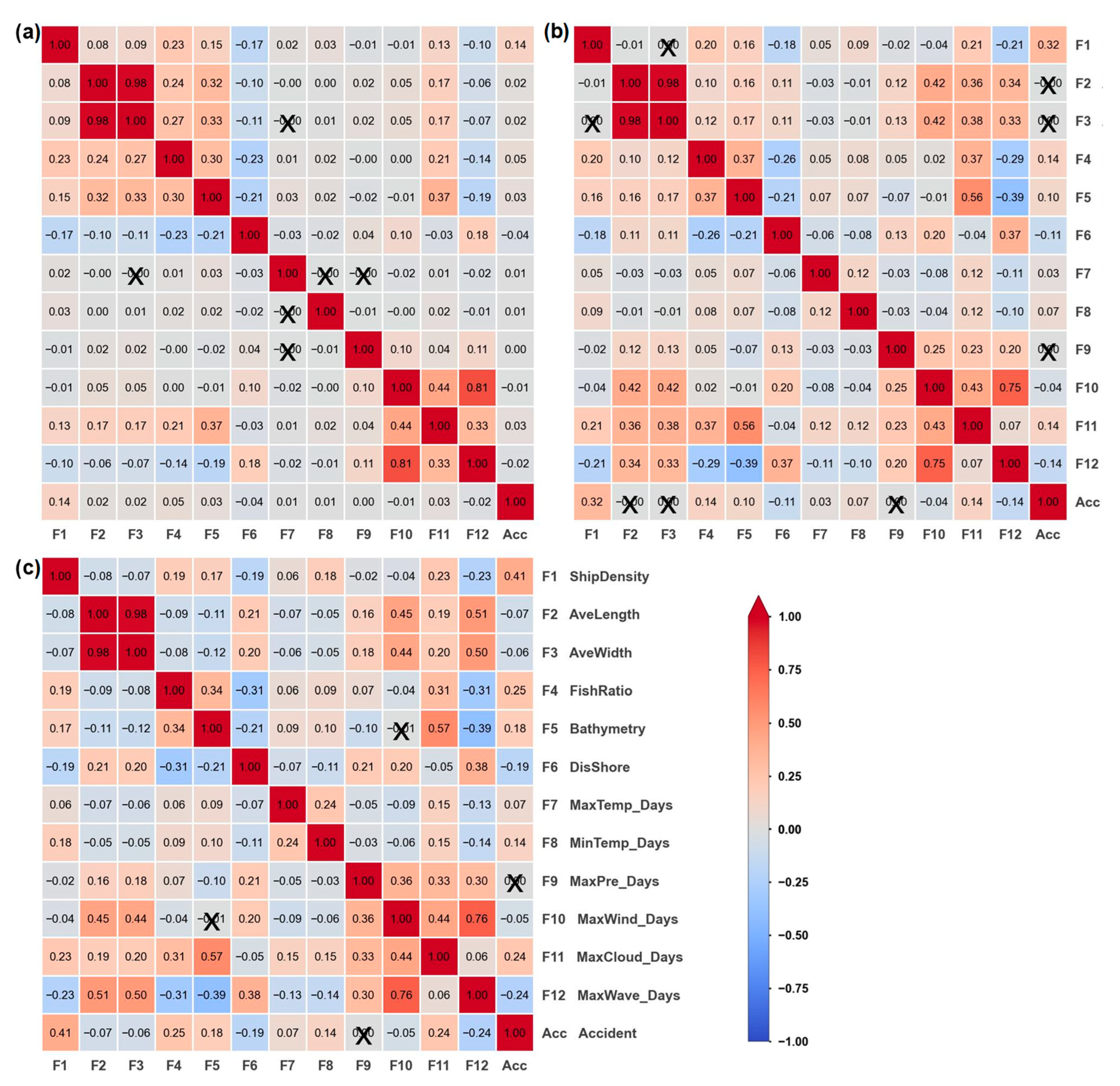
4.1. Correlation Analysis of Explanatory Factors
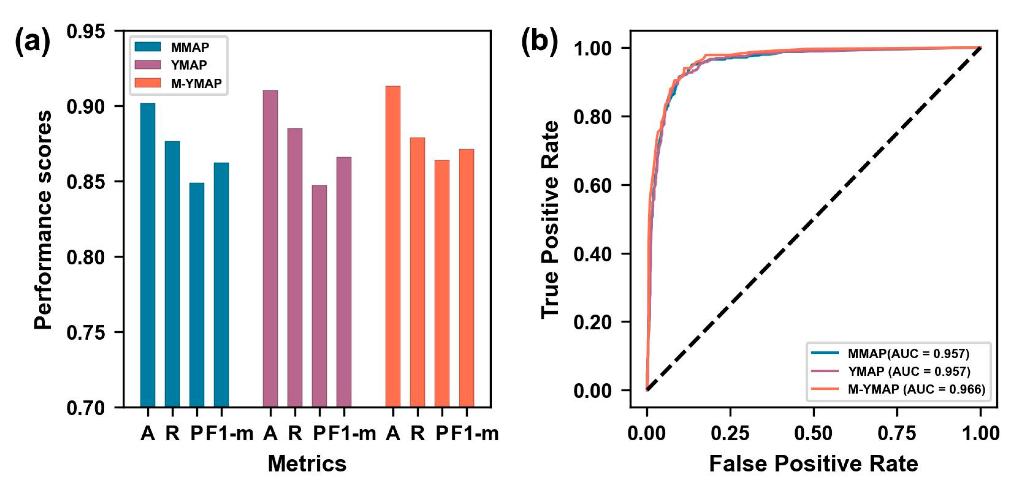
4.2. Model Performance Analysis
4.3. Generation of Accident Susceptibility Maps
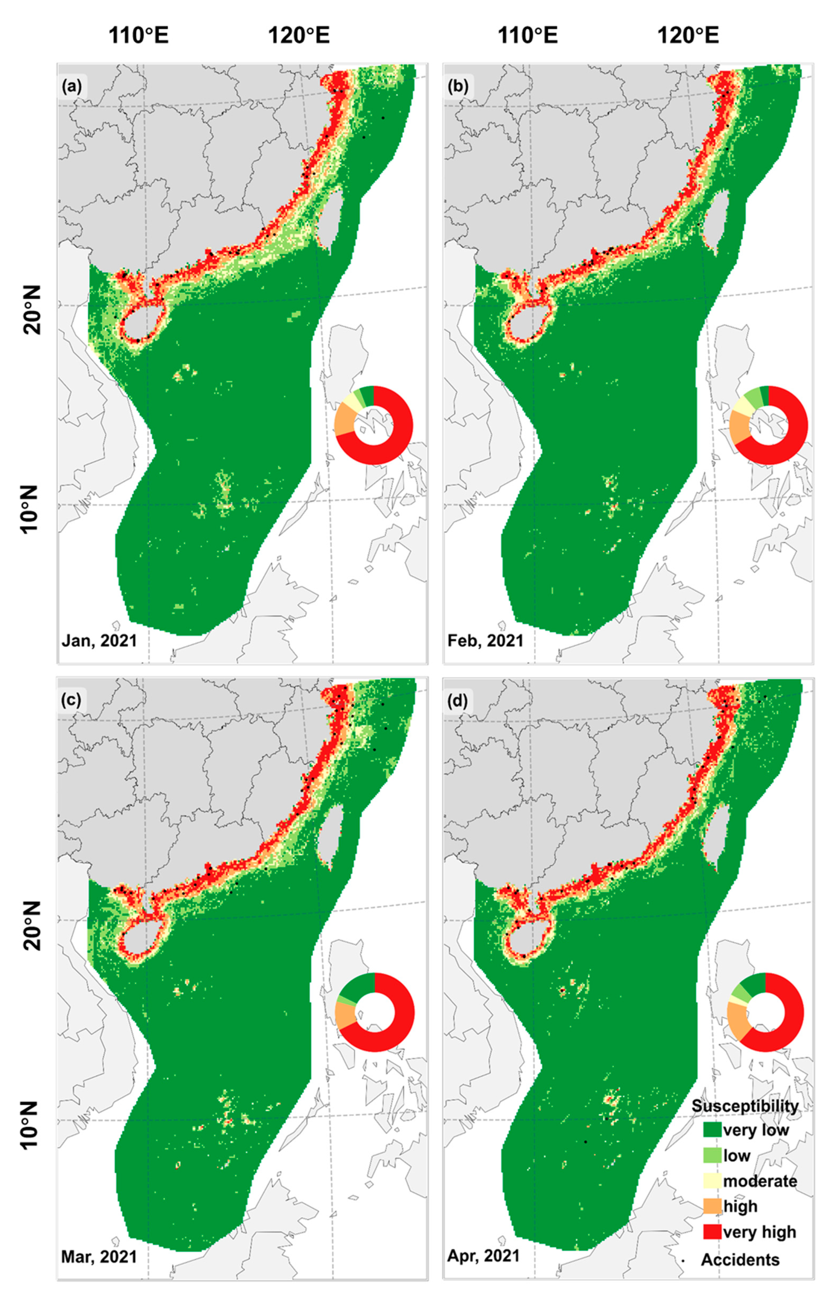
4.3.1. Generation of Accident Susceptibility Maps
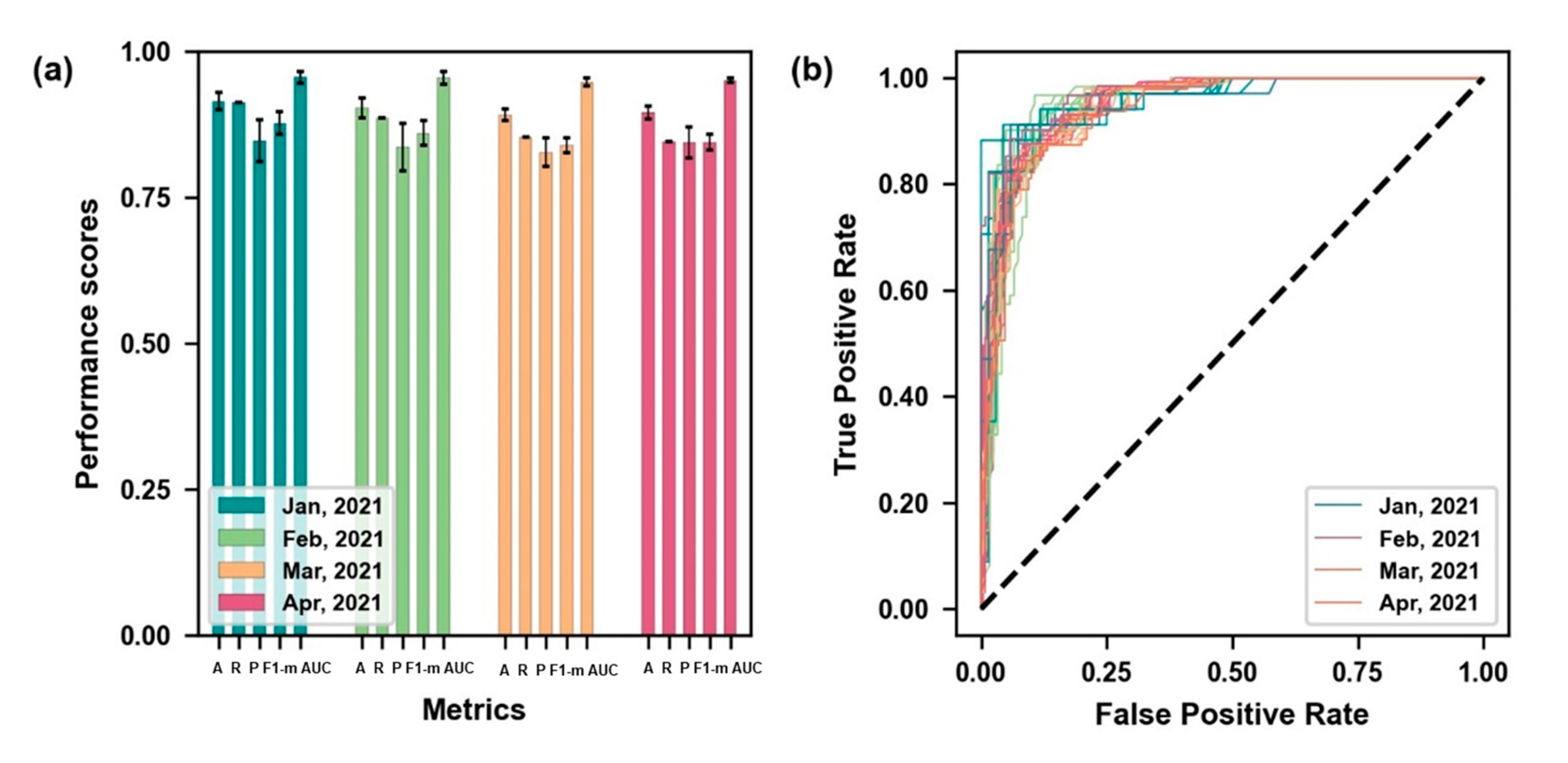
4.3.2. Generation of Accident Susceptibility for Blind Data
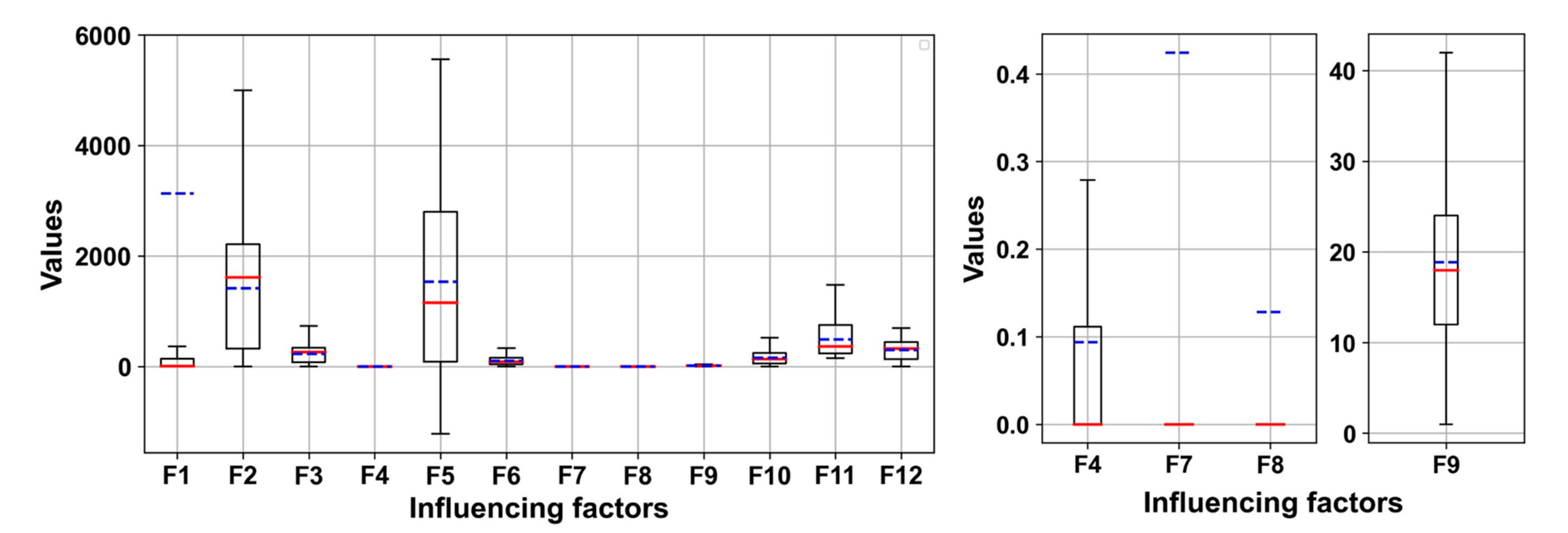
4.4. Influencing Factor Analysis
5. Discussion
5.1. Cost–Benefit Analysis
5.2. The Limitations of This Study
6. Conclusions
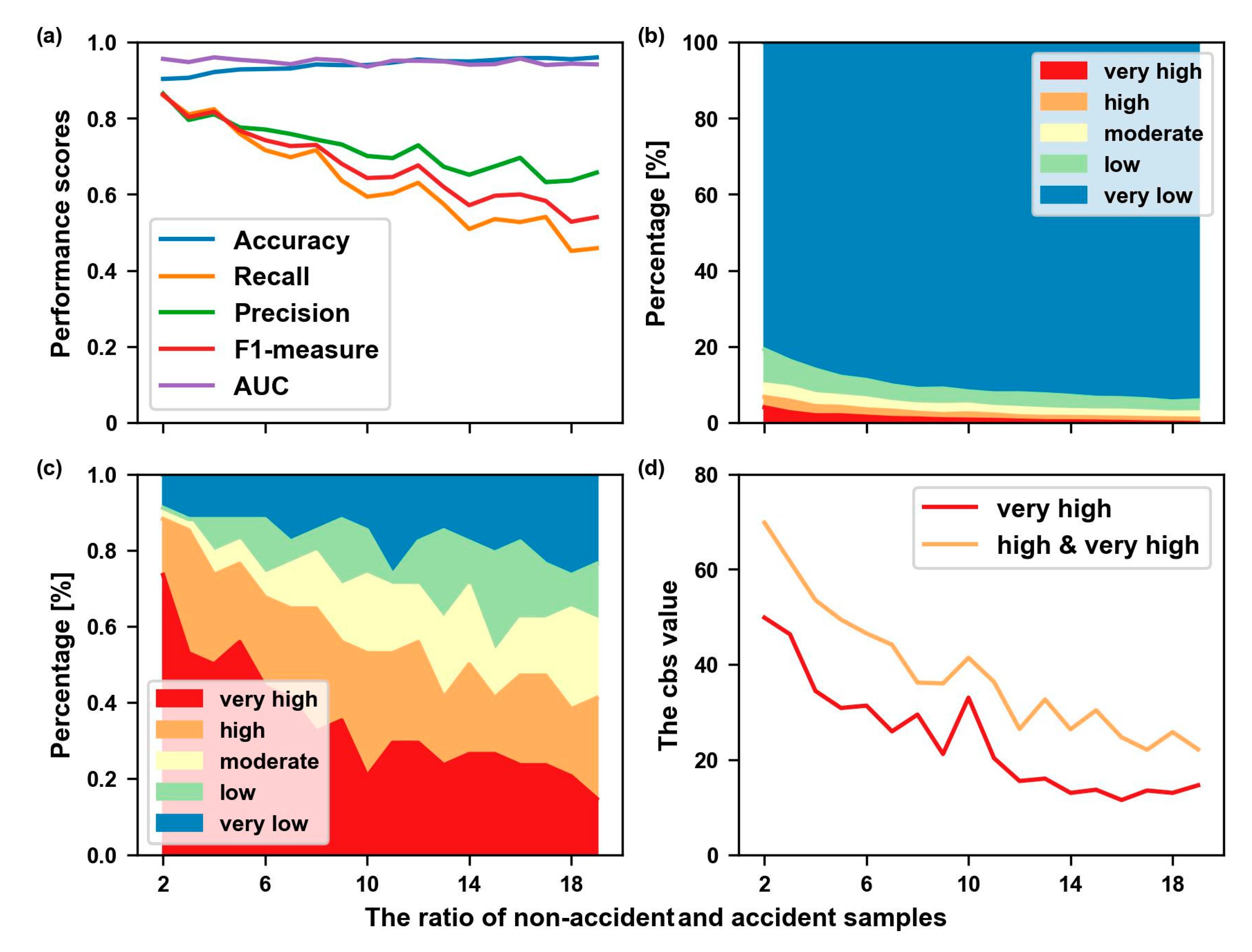
- The results showed good performances according to the accuracy, recall, precision, F1- measure, ROC, and AUC values in the testing data and blind data;
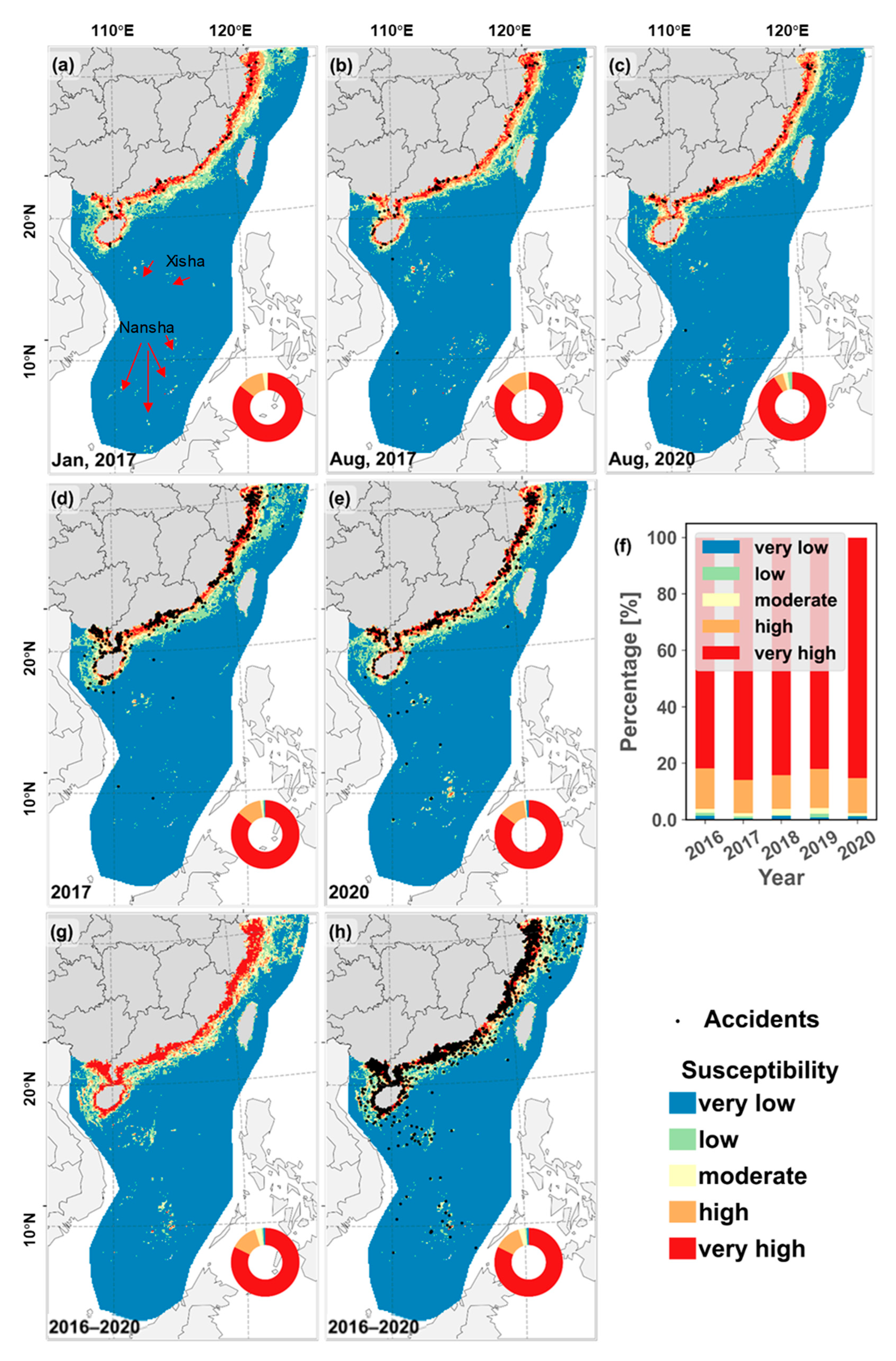
- In addition, the monthly, yearly, and five-yearly susceptibility maps show similar patterns. The high-susceptibility areas are close to the shore, especially from the Shanghai shore to the Guangxi shore;
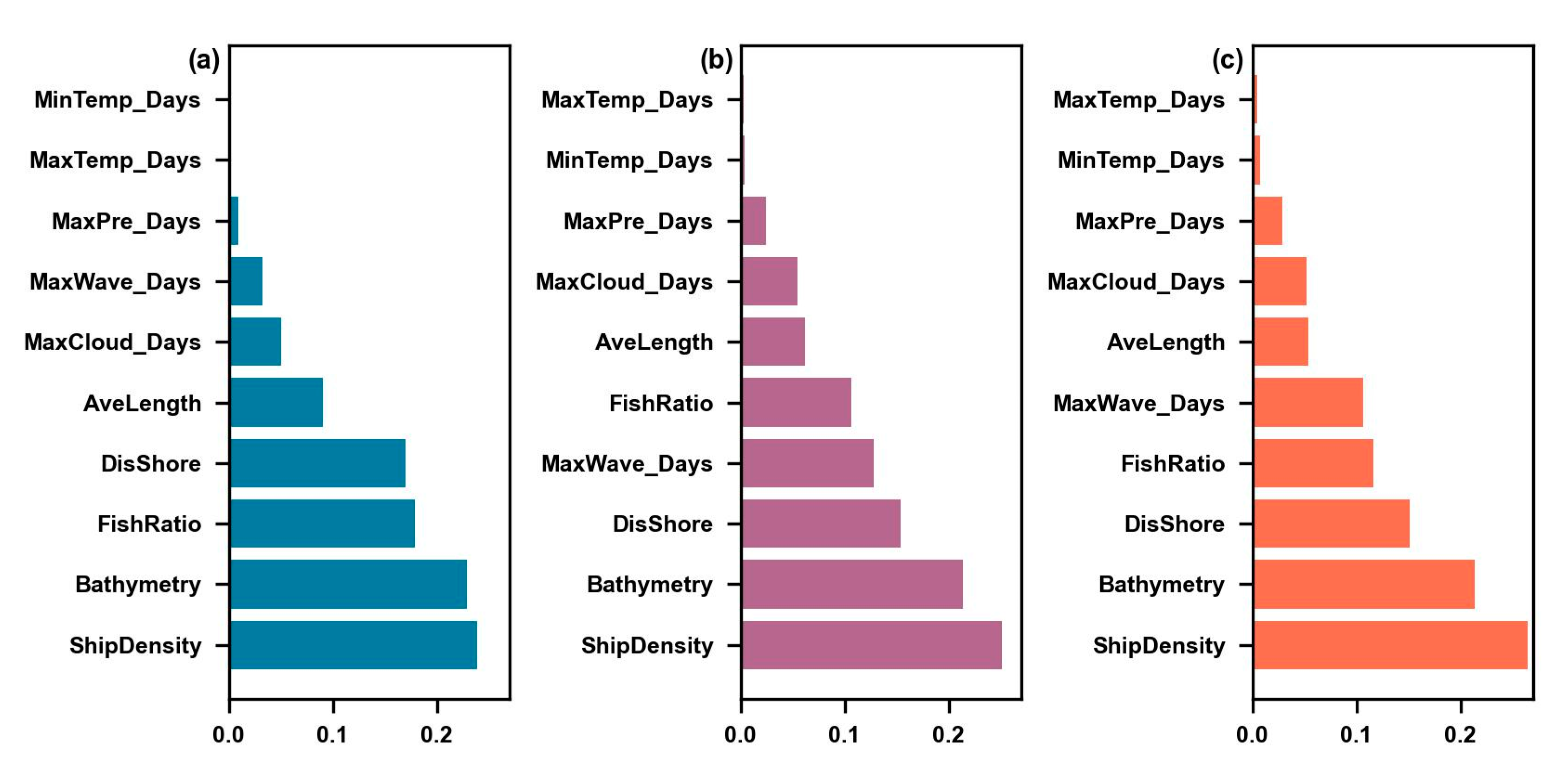
- Meanwhile, the conditioning factors in the three models had similar sorting. The ship density and bathymetry were the most critical factors in the three models, contributing around 25% and 20% of the total information.
Author Contributions
Funding
Institutional Review Board Statement
Informed Consent Statement
Data Availability Statement
Conflicts of Interest
Appendix A

| Variable | Description |
|---|---|
| AIS | Automatic Identification System |
| RF | Random forest |
| A | Accuracy metric |
| R | Recall metric |
| P | Precision metric |
| F1-m | F1-measure metric |
| ROC | Receiver operating characteristic curve |
| AUC values | Area under the ROC curve |
| MMAP | Monthly maritime accident prediction model |
| YMAP | Yearly maritime accident prediction model |
| M-YMAP | Multi-yearly maritime accident prediction model |
| VTS | Vessel Traffic Service |
| pyais PyPI | Python Pyais package |
| MSA | Maritime Safety Administration |
| Influencing factor | |
| Influencing factor | |
| The correlation coefficient between factor and factor | |
| The mean value of factor | |
| The mean value of factor | |
| The sample standard deviations of factor | |
| The sample standard deviations of factor | |
| The number of samples | |
| The sample, k = 1, 2, 3, …, . | |
| TP | True positive |
| TN | True negative |
| FP | False positive |
| FN | False negative |
| H-class | Very high–high-susceptibility class |
| cbr | Cost–benefit ratio |
| Susceptibility class s | |
| Cost–benefit ratio of susceptibility class s | |
| The number of accidents in class s | |
| The number of non-accident grids in class s | |
| Acc | Accident |
| F1–F12 | The abbreviations for influencing factors, which can be found in Table 1 |
| Month | Others | Collision | Sank | Stranding | Fire and Explosion | Touch Rocks | Wind | Touch | Damage by Waves | Operational Pollution |
|---|---|---|---|---|---|---|---|---|---|---|
| 1 | 108 | 48 | 38 | 38 | 21 | 11 | 3 | 4 | 2 | 1 |
| 2 | 83 | 27 | 28 | 31 | 22 | 10 | 0 | 3 | 1 | 0 |
| 3 | 98 | 69 | 34 | 46 | 24 | 16 | 1 | 10 | 0 | 2 |
| 4 | 108 | 66 | 41 | 35 | 10 | 16 | 7 | 8 | 0 | 1 |
| 5 | 98 | 38 | 32 | 26 | 18 | 7 | 3 | 2 | 1 | 1 |
| 6 | 105 | 24 | 28 | 35 | 12 | 7 | 1 | 3 | 2 | 2 |
| 7 | 125 | 25 | 43 | 44 | 18 | 16 | 21 | 4 | 9 | 2 |
| 8 | 161 | 66 | 37 | 42 | 27 | 23 | 32 | 5 | 3 | 2 |
| 9 | 126 | 70 | 42 | 51 | 28 | 25 | 9 | 4 | 5 | 0 |
| 10 | 150 | 61 | 56 | 50 | 24 | 23 | 15 | 3 | 3 | 2 |
| 11 | 100 | 53 | 44 | 30 | 20 | 11 | 2 | 3 | 4 | 1 |
| 12 | 144 | 50 | 51 | 31 | 11 | 23 | 3 | 5 | 3 | 1 |
References
- UNCTAD. Review of Maritime Transport 2022. Available online: https://unctad.org/rmt2022 (accessed on 10 August 2023).
- Rawson, A.; Brito, M.; Sabeur, Z.; Tran-Thanh, L. A Machine Learning Approach for Monitoring Ship Safety in Extreme Weather Events. Saf. Sci. 2021, 141, 105336. [Google Scholar] [CrossRef]
- Yang, Y.; Shao, Z.; Hu, Y.; Mei, Q.; Pan, J.; Song, R.; Wang, P. Geographical Spatial Analysis and Risk Prediction Based on Machine Learning for Maritime Traffic Accidents: A Case Study of Fujian Sea Area. Ocean Eng. 2022, 266, 113106. [Google Scholar] [CrossRef]
- Ministry of Transport (MOT), Measures for the Statistics of Maritime Accidents; 2021. Available online: https://www.gov.cn/zhengce/2021-09/01/content_5711528.htm (accessed on 19 May 2023).
- Yang, S. Analysis of Water Traffic Safety Situation in China; 2019 China International Ship Technology and Safety Forum, Beijing, China, 2019. Available online: https://www.cnss.com.cn/html/cnss/20190716/329008.html (accessed on 20 May 2023).
- Cao, Y.; Wang, M.; Liu, K. Wildfire Susceptibility Assessment in Southern China: A Comparison of Multiple Methods. Int. J. Disaster Risk Sci. 2017, 8, 164–181. [Google Scholar] [CrossRef]
- Van Dorp, J.R.; Merrick, J.R.W. On a Risk Management Analysis of Oil Spill Risk Using Maritime Transportation System Simulation. Ann. Oper. Res. 2011, 187, 249–277. [Google Scholar] [CrossRef]
- Huang, X.; Wen, Y.; Zhang, F.; Han, H.; Huang, Y.; Sui, Z. A Review on Risk Assessment Methods for Maritime Transport. Ocean Eng. 2023, 279, 114577. [Google Scholar] [CrossRef]
- Lois, P.; Wang, J.; Wall, A.; Ruxton, T. Formal Safety Assessment of Cruise Ships. Tour. Manag. 2004, 25, 93–109. [Google Scholar] [CrossRef]
- Mentes, A.; Akyildiz, H.; Yetkin, M.; Turkoglu, N. A FSA Based Fuzzy DEMATEL Approach for Risk Assessment of Cargo Ships at Coasts and Open Seas of Turkey. Saf. Sci. 2015, 79, 1–10. [Google Scholar] [CrossRef]
- Aydin, M.; Arici, S.S.; Akyuz, E.; Arslan, O. A Probabilistic Risk Assessment for Asphyxiation during Gas Inerting Process in Chemical Tanker Ship. Process Saf. Environ. Prot. 2021, 155, 532–542. [Google Scholar] [CrossRef]
- Faghih-Roohi, S.; Xie, M.; Ng, K.M. Accident Risk Assessment in Marine Transportation via Markov Modelling and Markov Chain Monte Carlo Simulation. Available online: http://worldcat.org/issn/00298018 (accessed on 11 August 2023).
- Hänninen, M.; Valdez Banda, O.A.; Kujala, P. Bayesian Network Model of Maritime Safety Management. Expert Syst. Appl. 2014, 41, 7837–7846. [Google Scholar] [CrossRef]
- Wang, L.; Yang, Z. Bayesian Network Modelling and Analysis of Accident Severity in Waterborne Transportation: A Case Study in China. Reliab. Eng. Syst. Saf. 2018, 180, 277–289. [Google Scholar] [CrossRef]
- Chang, Z.; He, X.; Fan, H.; Guan, W.; He, L. Leverage Bayesian Network and Fault Tree Method on Risk Assessment of LNG Maritime Transport Shipping Routes: Application to the China–Australia Route. J. Mar. Sci. Eng. 2023, 11, 1722. [Google Scholar] [CrossRef]
- Cem Kuzu, A.; Akyuz, E.; Arslan, O. Application of Fuzzy Fault Tree Analysis (FFTA) to Maritime Industry: A Risk Analysing of Ship Mooring Operation. Ocean Eng. 2019, 179, 128–134. [Google Scholar] [CrossRef]
- Wang, Y.; Fu, S. Framework for Process Analysis of Maritime Accidents Caused by the Unsafe Acts of Seafarers: A Case Study of Ship Collision. J. Mar. Sci. Eng. 2022, 10, 1793. [Google Scholar] [CrossRef]
- Rawson, A.; Brito, M.; Sabeur, Z. Spatial Modeling of Maritime Risk Using Machine Learning. Risk Anal. 2022, 42, 2291–2311. [Google Scholar] [CrossRef]
- Nourmohammadi, Z.; Nourmohammadi, F.; Kim, I.; Park, S.H. A Deep Spatiotemporal Approach in Maritime Accident Prediction: A Case Study of the Territorial Sea of South Korea. Ocean Eng. 2023, 270, 113565. [Google Scholar] [CrossRef]
- MSA, Maritime Safety Administration of the People’s Republic of China. Available online: https://www.msa.gov.cn/ (accessed on 15 August 2023).
- Breiman, L. Random Forests. Mach. Learn. 2001, 45, 5–32. [Google Scholar] [CrossRef]
- Stumpf, A.; Kerle, N. Object-Oriented Mapping of Landslides Using Random Forests. Remote Sens. Environ. 2011, 115, 2564–2577. [Google Scholar] [CrossRef]
- He, Q.; Wang, M.; Liu, K. Rapidly Assessing Earthquake-Induced Landslide Susceptibility on a Global Scale Using Random Forest. Geomorphology 2021, 391, 107889. [Google Scholar] [CrossRef]
- Li, B.; Liu, K.; Wang, M.; He, Q.; Jiang, Z.; Zhu, W.; Qiao, N. Global Dynamic Rainfall-Induced Landslide Susceptibility Mapping Using Machine Learning. Remote Sens. 2022, 14, 5795. [Google Scholar] [CrossRef]
- Du, G.; Zhang, Y.; Iqbal, J.; Yang, Z.; Yao, X. Landslide Susceptibility Mapping Using an Integrated Model of Information Value Method and Logistic Regression in the Bailongjiang Watershed, Gansu Province, China. J. Mt. Sci. 2017, 14, 249–268. [Google Scholar] [CrossRef]
- Tien Bui, D.; Tuan, T.A.; Klempe, H.; Pradhan, B.; Revhaug, I. Spatial Prediction Models for Shallow Landslide Hazards: A Comparative Assessment of the Efficacy of Support Vector Machines, Artificial Neural Networks, Kernel Logistic Regression, and Logistic Model Tree. Landslides 2016, 13, 361–378. [Google Scholar] [CrossRef]
- Marceau, L.; Qiu, L.; Vandewiele, N.; Charton, E. A Comparison of Deep Learning Performances with Other Machine Learning Algorithms on Credit Scoring Unbalanced Data. arXiv 2020, arXiv:1907.12363. [Google Scholar]
- Merghadi, A.; Yunus, A.P.; Dou, J.; Whiteley, J.; ThaiPham, B.; Bui, D.T.; Avtar, R.; Abderrahmane, B. Machine Learning Methods for Landslide Susceptibility Studies: A Comparative Overview of Algorithm Performance. Earth-Sci. Rev. 2020, 207, 103225. [Google Scholar] [CrossRef]
- Lv, P.; Zhuang, Y.; Yang, K. Prediction of Ship Traffic Flow Based on BP Neural Network and Markov Model. MATEC Web Conf. 2016, 81, 04007. [Google Scholar] [CrossRef]
- Kashyap, A.A.; Raviraj, S.; Devarakonda, A.; Nayak K, S.R.; Venkata, S.K.; Bhat, S.J. Traffic Flow Prediction Models—A Review of Deep Learning Techniques. Cogent Eng. 2022, 9, 2010510. [Google Scholar] [CrossRef]


| No. | Data | Resolution (Original) | Unit | Description | Source |
|---|---|---|---|---|---|
| F1 | ShipDensity | - | pc | The number of ships in a unit | https://www.msa.gov.cn/ (accessed on 20 March 2023) |
| F2 | AveLength | - | m | The average length in a unit | https://www.msa.gov.cn/ (accessed on 20 March 2023) |
| F3 | AveWidth | - | m | The average width in a unit | https://www.msa.gov.cn/ (accessed on 20 March 2023) |
| F4 | FishRatio | - | ratio | The ratio of fishing vessels in a unit | https://www.msa.gov.cn/ (accessed on 20 March 2023) |
| F5 | Bathymetry | 1′ (~2 km) | m | The bathymetry of the grid | https://www.ngdc.noaa.gov/mgg/global/etopo5.HTML (accessed on 23 March 2023) |
| F6 | DisShore | - | km | The distance from shore | https://gadm.org/download_world.html (accessed on 24 March 2023) |
| F7 | MaxTemp_Days | 0.25° (~27 km) | °C | The number of days of temperatures exceeding 35 °C | https://cds.climate.copernicus.eu/portfolio/dataset/reanalysis-era5-single-levels (accessed on 28 March 2023) |
| F8 | MinTemp_Days | 0.25° (~27 km) | °C | The number of days of temperatures lower than 0 °C | https://cds.climate.copernicus.eu/portfolio/dataset/reanalysis-era5-single-levels (accessed on 28 March 2023) |
| F9 | MaxPre_Days | 0.25° (~27 km) | mm | The number of days of precipitation exceeding 50 mm | https://cds.climate.copernicus.eu/portfolio/dataset/reanalysis-era5-single-levels (accessed on 28 March 2023) |
| F10 | MaxWind_Days | 0.25° (~27 km) | m/s | The number of days of the wind speed exceeding 17.2 m/s | https://cds.climate.copernicus.eu/portfolio/dataset/reanalysis-era5-single-levels (accessed on 28 March 2023) |
| F11 | Maxcloud_Days | 0.25° (~27 km) | ratio | The number of days of the cloud height exceeding 0.8 | https://cds.climate.copernicus.eu/portfolio/dataset/reanalysis-era5-single-levels (accessed on 28 March 2023) |
| F12 | MaxWave_Days | 0.25° (~27 km) | m | The number of days of the wave height exceeding 2.5 m | https://cds.climate.copernicus.eu/portfolio/dataset/reanalysis-era5-single-levels (accessed on 28 March 2023) |
Disclaimer/Publisher’s Note: The statements, opinions and data contained in all publications are solely those of the individual author(s) and contributor(s) and not of MDPI and/or the editor(s). MDPI and/or the editor(s) disclaim responsibility for any injury to people or property resulting from any ideas, methods, instructions or products referred to in the content. |
© 2023 by the authors. Licensee MDPI, Basel, Switzerland. This article is an open access article distributed under the terms and conditions of the Creative Commons Attribution (CC BY) license (https://creativecommons.org/licenses/by/4.0/).
Share and Cite
Zhu, W.; Wang, S.; Liu, S.; Yang, L.; Zheng, X.; Li, B.; Zhang, L. Dynamic Multi-Period Maritime Accident Susceptibility Assessment Based on AIS Data and Random Forest Model. J. Mar. Sci. Eng. 2023, 11, 1935. https://doi.org/10.3390/jmse11101935
Zhu W, Wang S, Liu S, Yang L, Zheng X, Li B, Zhang L. Dynamic Multi-Period Maritime Accident Susceptibility Assessment Based on AIS Data and Random Forest Model. Journal of Marine Science and Engineering. 2023; 11(10):1935. https://doi.org/10.3390/jmse11101935
Chicago/Turabian StyleZhu, Weihua, Shoudong Wang, Shengli Liu, Libo Yang, Xinrui Zheng, Bohao Li, and Lixiao Zhang. 2023. "Dynamic Multi-Period Maritime Accident Susceptibility Assessment Based on AIS Data and Random Forest Model" Journal of Marine Science and Engineering 11, no. 10: 1935. https://doi.org/10.3390/jmse11101935
APA StyleZhu, W., Wang, S., Liu, S., Yang, L., Zheng, X., Li, B., & Zhang, L. (2023). Dynamic Multi-Period Maritime Accident Susceptibility Assessment Based on AIS Data and Random Forest Model. Journal of Marine Science and Engineering, 11(10), 1935. https://doi.org/10.3390/jmse11101935