Article

Magnetic Gradient Tensor Positioning Method Implemented on an Autonomous Underwater Vehicle Platform

1
School of Mechanical Engineering, Hangzhou Dianzi University, Hangzhou 310018, China
2
Ocean Technology and Equipment Research Center, Hangzhou Dianzi University, Hangzhou 310018, China
3
School of Electronics and Information Engineering, Hangzhou Dianzi University, Hangzhou 310018, China
4
Tianjin Huiyang Intelligent Equipment Co., Ltd., Tianjin 300384, China
*
Authors to whom correspondence should be addressed.
J. Mar. Sci. Eng. 2023, 11(10), 1909; https://doi.org/10.3390/jmse11101909
Submission received: 11 September 2023 / Revised: 27 September 2023 / Accepted: 29 September 2023 / Published: 2 October 2023
(This article belongs to the Section Physical Oceanography)

Abstract

:
Underwater magnetic surveying serves as the fundamental prerequisite for detecting sensitive underwater targets and magnetically susceptible submerged objects. However, when utilizing magnetic gradient tensor measurements for underwater positioning, the stability of the measurement apparatus can be significantly affected by hydrodynamic disturbances in the underwater environment, thereby having a substantial impact on data quality. Autonomous Underwater Vehicles (AUV) are unmanned underwater robots designed to independently perform various tasks and operations in underwater environments. In order to ensure the quality of data collection, this paper proposes a structure utilizing an Autonomous Underwater Vehicles platform equipped with a three-component magnetic gradiometer. This structure employs second-order tensor positioning algorithms and vertical gradient positioning algorithms, coupled with the Autonomous Underwater Vehicles’s inherent vertical profile motion, to effectively achieve the precise positioning of underwater cables. Simulation results indicate that, in the absence of geomagnetic background noise, both horizontal and vertical structures yield favorable positioning results. However, when introducing background noise of 40,000 nT, the horizontal structure exhibits larger positioning errors, whereas the vertical structure demonstrates smaller errors. Experimental results show that in near-field scenarios, both structures achieve relatively similar positioning accuracy. Nevertheless, under identical distances in the far field, the vertical structure reduces errors by a minimum of 30.78% compared to the horizontal structure, thereby confirming the feasibility of integrating magnetic gradient tensor measurement structures with Autonomous Underwater Vehicles platforms.

1. Introduction

Currently, undersea cables are primarily used for transoceanic power transmission and transoceanic communication. However, geological activities and marine life can pose a certain level of damage to these cables. If undersea optical cables are seriously damaged, it can result in incalculable losses to national economic activities. Therefore, it is crucial to have a fast cable repair mechanism [1]. Additionally, rapid cable location can significantly improve the efficiency of cable maintenance. Furthermore, the development of marine resources [2] has always been an important issue that plays a significant role in economic development. However, traditional optical methods have substantial limitations [3], such as color distortion and low visibility. Hence, there is an urgent need in related fields for an effective means of detecting underwater resources. In the vicinity of ferromagnetic materials and energized underwater cables [4], specific magnetic fields are generated. The characteristics of these magnetic fields are influenced by the objects’ geometric properties, material composition, frequency attributes of the current, magnitude, and orientation. Consequently, it is possible to deduce various types of information about the target objects from these magnetic fields, including details about their position, orientation, and structural attributes. Underwater magnetic field environments are generally more stable compared to those on land, making magnetic exploration techniques more reliable and stable for underwater applications. Compared to the currently prevalent acoustic detection methods, which exhibit a higher susceptibility to false positives in specific environments [5], magnetic exploration techniques have been gaining increasing attention for detecting submerged magnetic targets due to their fundamental resistance to the influence of factors like water bodies and sedimentary materials [6]. Magnetic anomaly detection involves the collection of magnetic field information within a localized area using sensors, followed by the analysis of magnetic anomaly signals. This process aims to identify a range of magnetic targets [7,8,9]. Magnetic anomaly detection can be divided into two approaches: incorporating digital signal processing methods into magnetic anomaly data processing, such as detection algorithms based on standard orthogonal basis function decomposition [10], and introducing magnetic gradient tensor matrices, which is currently a hot topic in this research field. Previous studies have mostly focused on the utilization of the magnetic gradient tensor matrix itself and the matrix’s eigenvalues and eigenvectors. The magnetic gradient tensor refers to the first-order gradient tensor of the three components of the magnetic field vector in three-dimensional space [11]. Relative to magnetic field scalar and vector measurements, the magnetic gradient tensor contains more comprehensive magnetic field information and can effectively mitigate background noise from the Earth’s magnetic field, thus offering distinct advantages in magnetic anomaly measurements [12]. Currently, research based on the magnetic gradient tensor is primarily applied to the identification, detection, and localization of underwater mineral deposits and sensitive underwater targets [13,14,15].
For the localization of underwater magnetic targets, when the relative distance between the magnetic target and the magnetic sensor array is greater than 2.5 times, the magnetic target can be approximated as a magnetic dipole [16]. Current positioning algorithms can be broadly categorized into two approaches: magnetic localization based on single-point magnetic data acquisition and iterative estimation of position vectors using multi-point magnetic data, yielding an approximate solution. Building upon the magnetic dipole model, Nara [17] introduced a positioning method based on the magnetic gradient tensor. This approach involves computing the magnetic gradient tensor matrix of the sensor array along with the three components of the magnetic field. By performing these calculations, the relative position information between the magnetic source and the sensor array can be determined. As a derivative, WANG [18] discovered that measurement calculation errors of the magnetic gradient tensor matrix affect positioning errors and made certain corrections to it, achieving good results to some extent. Although this algorithm can directly solve for position information during the computation, it incorporates the Earth’s geomagnetic background field. If the magnetic anomaly generated by the magnetic target due to magnetization by the geomagnetic field is smaller than or close to the noise of the geomagnetic background field, the accuracy of this computational model’s localization can be significantly impacted. In practical applications, it is challenging to extract the three-component magnetic field and total field information of target objects from acquired magnetic field data unless the background magnetic field within the measurement area is known in advance. Hence, future research efforts will primarily focus on mitigating the influence of the background magnetic field. Wiegert [19] designed a magnetic gradiometer structure. This structure measures three magnetic gradient components, and by comparing their magnitudes, it estimates the approximate direction of the target object. However, the presence of ellipsoid errors has led to less-than-ideal results in terms of accuracy and performance. G. Iacca and G. YIN [20,21] proposed a multi-point iterative positioning algorithm in their computational model. In this computational model, the influence of the geomagnetic field is eliminated through multiple points, but solving for position information requires the use of iterative algorithms [22,23] to solve nonlinear equations. Liu [24] introduced magnetic moment constraints to the multi-point iterative positioning algorithm. By adding a penalty coefficient to the objective function, this approach can ensure positioning accuracy even when sensor accuracy is low. However, positioning accuracy is somewhat related to the penalty coefficient, resulting in some degree of uncertainty. The multi-point iterative algorithm consumes a significant amount of time in computation, and in practical applications, there may be some latency. It can be challenging to meet real-time requirements in certain specific applications that demand high real-time performance. Li [25] proposed a positioning algorithm based on the eigenvalues and eigenvectors of the magnetic gradient tensor. However, this method can yield four possible target position vectors in a single measurement, requiring additional error elimination techniques. YU ZH T [26] introduced a positioning algorithm involving the first-order differentiation of the magnetic gradient along the Z-axis direction. This model includes the first-order tensor of the magnetic field’s gradient along the vertical direction and the first-order differentiation of the magnetic gradient tensor along the vertical direction. Importantly, this model excludes the geomagnetic background field, and the impact of geomagnetic noise on this computational model is relatively minor. However, this model utilizes the second-order component of the geomagnetic field along the Z-axis, imposing strict requirements on the measurement device’s structural design.
During the process of practical detection, the instability of the hydrodynamic environment in the ocean, both in terms of time and space, poses a significant challenge to maintaining the orientation stability of the underwater magnetic measurement apparatus. This vulnerability results in a sharp deterioration in the quality of collected data. Moreover, potential interference from other magnetic sources within the magnetic surveying environment can further compound these challenges. Consequently, there is a strong demand for ensuring the stability of the measurement system’s orientation and minimizing the impact of external magnetic interference during magnetic surveys. With the evolution of underwater vehicles, their inherent characteristics of stability and autonomous operation have found widespread application in the field of underwater exploration [27]. Equipping underwater vehicles with arrays of three-component fluxgate magnetometers ensures range measurements while minimizing orientation errors. This approach guarantees high-quality data acquisition by addressing both stability and interference issues simultaneously.
Building upon the aforementioned research, this paper proposes a modification to the original algorithm. By taking advantage of the AUV’s vertical motion capabilities [28,29], the regular hexahedral array is transformed into a triangular array, which is more feasible to implement on an AUV. Additionally, a planar array is dynamically utilized to achieve a three-dimensional array configuration, meeting the differentiation requirements along the z-axis [30,31]. As a result, compared to the original algorithm, this modification aims to minimize the attitude errors introduced by manual manipulation and reduce interference from other magnetic sources [32], thereby enhancing the quality of data collection.
The organization of this paper is as follows. Section 2 introduces the theoretical foundation of magnetic gradient tensors and presents the magnetic gradient tensor localization algorithm based on single-point measurements. It also discusses the magnetic gradient tensor localization algorithm incorporating the AUV platform’s vertical profiling capabilities. Section 3 provides simulation and experimental results and conducts an in-depth analysis of these outcomes. Section 4 discusses how to enhance the accuracy of the altitude-based positioning algorithm on the AUV platform and compares it with other algorithms. Section 5 discusses the implications of this work and outlines potential directions for future research.

2. Magnetic Gradient Tensor Localization Theory

2.1. Magnetic Gradient Tensor

The geomagnetic field consists of three component fields, with projections onto the X-axis component B x , Y-axis component B y , and Z-axis component B z and the Cartesian coordinate system, respectively:
B = B x B y B z T .
The magnetic field data collected in practical scenarios often take the form of B = B 0 + B a + φ , where B 0 represents the background magnetic field, B a signifies the magnetic anomaly field generated by ferromagnetic objects or objects capable of inducing magnetic disturbances, and φ represents the noise introduced by the onboard sensors and circuitry, along with the magnetic field fluctuations. The three components of the collected magnetic field data also adhere to the aforementioned format.
A tensor is a matrix that increases from lower dimensions to higher dimensions. The magnetic gradient tensor refers to the rate of change of the three aforementioned components along the three directions in the Cartesian coordinate system. It comprises nine elements forming a matrix known as the magnetic gradient tensor matrix. Its expression is as follows:
G = B x x B x y B x z B y x B y y B y z B z x B z y B z z .
In a source-free field, the divergence and curl of the magnetic field are both equal to zero. This can be deduced from Maxwell’s equations:
· B = δ B x δ x + δ B y δ y + δ B z δ z
× B = i j k δ δ x δ δ y δ δ z B x B y B z = 0 .
Further derivation of the above equation yields:
t r ( G ) = 0 B x y = B y x B x z = B z x B y z = B z y .
Combining Equation (5), it can be observed that out of the nine elements in the magnetic gradient tensor matrix, only five elements are independent. Consequently, Equation (2) can be transformed into:
G = B x x B x y B x z B x y B y y B y z B x z B y z ( B x x + B y y ) .

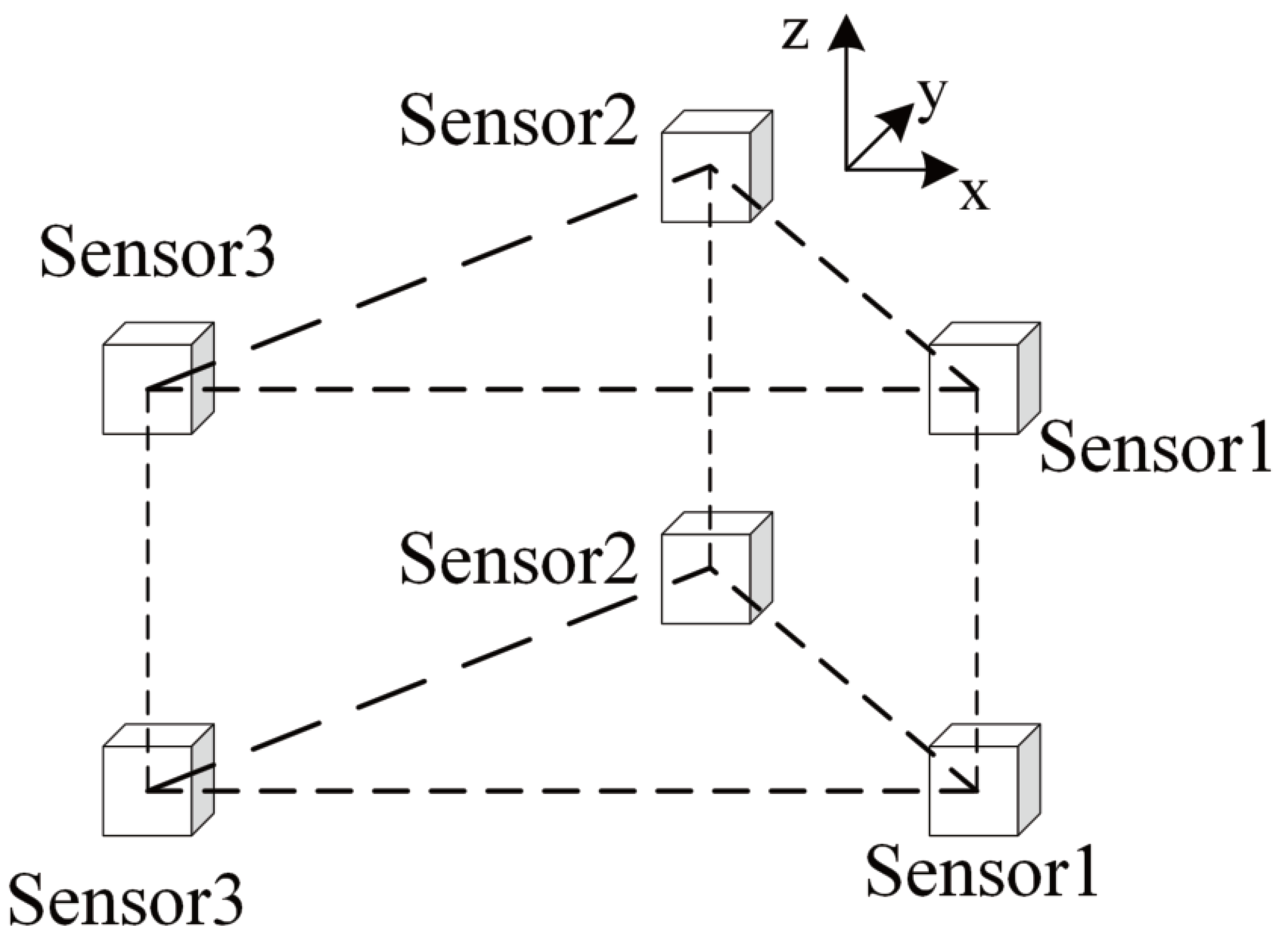
2.2. Magnetic Gradient Tensor Structure and Localization Model Based on AUV Platform

2.2.1. Horizontal Magnetic Gradient Tensor Structure and Its Localization Model

The horizontal magnetic gradient tensor structure is illustrated in Figure 1, with three fluxgate magnetometer sensors arranged horizontally on the AUV. The Y-axis of the magnetic sensor array is parallel to the AUV’s bow direction. Among them, the three-component outputs of the magnetic sensors are denoted as B i j , where it represents the sensor number. It is established that the right fluxgate magnetometer sensor is Sensor 1, the front-facing sensor is Sensor 2, and the left fluxgate magnetometer sensor is Sensor 3. j = x , y , z represents the component field of a sensor. The tensor expression for this structure at the origin can be represented in matrix form as follows:
a 11 a 12 a 13 a 21 a 22 a 23 a 31 a 32 a 33
a 11 = 1 d 1 B 1 x B 3 x
a 12 = 1 d 1 B 1 y B 3 y
a 13 = 1 d 1 B 1 z B 3 z
a 21 = 1 d 1 B 1 y B 3 y
a 22 = 1 d 2 B 2 y 1 2 ( B 1 y + B 3 y )
a 23 = 1 d 2 B 2 z 1 2 ( B 1 z + B 3 z )
a 31 = 1 d 1 B 1 z B 3 z
a 32 = 1 d 2 B 2 z 1 2 ( B 1 z + B 3 z )
a 33 = ( a 11 + a 22 ) ,
where d 1 is the distance between Sensor 1 and Sensor 3, referred to as Baseline 1; taking the midpoint between Sensor 1 and Sensor 3 as point C, d 2 is the distance be-tween Sensor 2 and point C, termed Baseline 2.
When the detection distance is more than 2.5 times the size of the magnetic target, the magnetic target under investigation can be treated as a magnetic dipole. Through the magnetic dipole model, the localization of the magnetic target can be achieved. The magnetic field intensity at a distance from the magnetic target is given by:
B = 3 μ 0 ( m · r 0 ) r 0 μ 0 m 4 π r 3 .
In the equation, m ( A · m ) represents the magnetic moment of the magnetic target; μ 0 stands for the vacuum permeability, with a magnitude of 4 π × 10 7 ( H / m ) ; r = | r | represents the distance from the magnetic target to the sensor array; r 0 is a unit vector of r .
The magnetic field B at point A can be represented as:
B = 3 μ 0 ( m · r 0 ) r 0 μ 0 m 4 π ( r + d r ) 3 .
Thus:
B B = 3 r 3 μ 0 ( m · r 0 ) r 0 μ 0 m 4 π r 3 d r .
Furthermore:
B B = δ B x δ x δ B x δ y δ B x δ z δ B y δ x δ B y δ y δ B y δ z δ B z δ x δ B z δ y δ B z δ z · r 0 d r .
Combining Equation (10) with Equation (11), we obtain:
G r = 3 B .
Namely:
r = x y z = 3 B x x B x y B x z B y x B y y B y z B z x B z y B z z 1 B x B y B z .
Equation (13) represents the single-point localization formula based on the magnetic gradient tensor. In theory, obtaining the magnetic gradient tensor at a specific point in space and the three-component magnetic field strength should enable magnetic source localization. However, due to the relatively ideal magnetic field environment underwater, the gradient of the background field can be considered to be approximately zero. In practical measurements, there exists a certain measurement error in estimating the background field, which may result in some residual background field in Equation (13). In the near-field scenario, where the magnetic field signal generated by the target object is relatively strong and not completely submerged within the background field, the localization error can be considered reasonably reliable. However, in the far-field scenario, the signal-to-noise ratio of the data collected by sensors is relatively poor, which could lead to larger localization errors.

2.2.2. Vertical Magnetic Gradient Tensor Structure and Its Localization Model

Due to the significant error introduced by the Earth’s magnetic field in the single-point localization formula based on magnetic gradient tensor, this paper combines the characteristics of underwater cables and leverages the advantages of AUVs maintaining multiple orientations in underwater magnetic survey applications. By adopting a vertical gradient approach for positioning, as depicted in Figure 2, the magnetic field information collected by the AUV along different depth profiles is utilized to compute first-order and second-order tensors.
For Equation (12), taking partial derivatives with respect to the Z-direction on both sides of the equation yields:
δ B x x δ z r x + δ B x y δ z r y + δ B x z δ z r z + B x z δ r z δ z = 3 δ B x δ z δ B y x δ z r x + δ B y y δ z r y + δ B y z δ z r z + B y z δ r z δ z = 3 δ B y δ z δ B z x δ z r x + δ B z y δ z r y + δ B z z δ z r z + B z z δ r z δ z = 3 δ B z δ z .
Because in the above equation, the partial derivative of the Z-direction vector with respect to the Z-axis direction is a constant 1, the equation can be rewritten as:
δ B x x δ z r x + δ B x y δ z r y + δ B x z δ z r z = 4 δ B x δ z δ B y x δ z r x + δ B y y δ z r y + δ B y z δ z r z = 4 δ B y δ z δ B z x δ z r x + δ B z y δ z r y + δ B z z δ z r z = 4 δ B z δ z .
Namely,
r = x y z = 4 δ G δ z 1 δ B δ z .
Equation (16) represents the localization computation model based on the vertical gradient tensor. This algorithm replaces the significant impact of the Earth’s magnetic field with the first-order tensor of the magnetic field in the vertical direction. Where δ B δ z represents the first-order tensor of the geomagnetic field along the Z-direction, and δ G δ z stands for the second-order tensor of the geomagnetic field along the Z-direction. In the equation, δ G δ z can be obtained through the difference between the two gradient tensors collected by the AUV’s magnetic survey array during vertical ascent and descent. Let the magnetic gradient tensor of the AUV on the upper horizontal profile be G T and the magnetic gradient tensor of the AUV on the lower horizontal profile be G B , then δ G δ z = G T G B Δ z , where Δ z is the vertical baseline, calculated from the depth sensor on the AUV.

2.2.3. Overall Approach of This Study

The vertical gradient algorithm proposed in this paper is illustrated in Figure 3. This method primarily involves using the AUV’s vertical ascent and descent movements to perform two rounds of magnetic data collection. Subsequently, vertical differencing is applied to the magnetic field intensities collected by the magnetic sensors, aiming to minimize the influence of the geomagnetic field, and calculate the partial derivative along the Z-axis of the magnetic gradient tensor matrices obtained from the two acquisitions. This process allows for the determination of the position information of magnetic targets. The time complexity of the vertical structure magnetic gradient algorithm in this paper is O(1). In a horizontal structure, it is necessary to first measure the numerical value of the background magnetic field and then estimate the magnetic anomaly field of the target object before incorporating it into Equation (13) for calculation.

3. Simulation and Experimentation

3.1. Structural Simulation Comparison

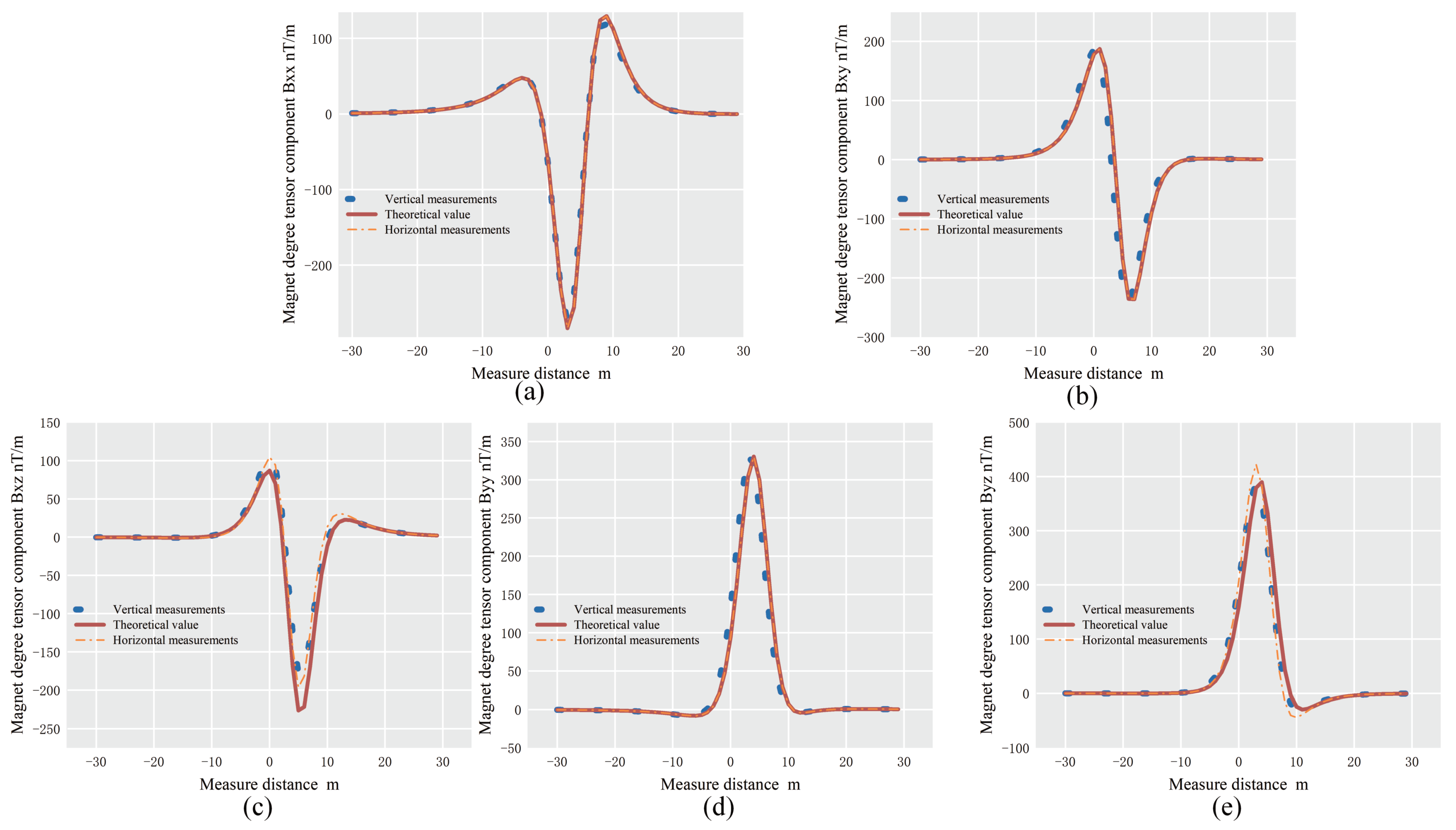
3.1.1. Comparison of Two Structural Tensor Simulations

To validate the feasibility of the horizontal magnetic gradient structure and the vertical magnetic gradient structure, gradient tensor simulations were conducted for both structures. The simulation conditions are outlined in Table 1.
The measured values of tensor components for both structures, along with the theoretical values of tensor components, are shown in Figure 4.
As shown in the figure, the measured values of both structures for each component are closely aligned with the fitted theoretical curves. Compared to the horizontal structure, the tensor measurements of the vertical gradient structure exhibit a closer alignment with the theoretical fitting curves.
In order to verify the accuracy of magnetic gradient tensor measurements for both structures, root mean square error ( R M S E ) was employed to assess the measurement results of the five tensors.
R M S E = 1 N i = 1 n ( G i T i ) 2 ( i = 1 , 2 , 3 , , N ) ,
where G i represents the gradient calculation value obtained from both structures at the same measurement point, T i is the theoretical gradient value at that point, and N is the number of measurement points.
The root mean square error data for each component is shown in Table 2. Combining the R M S E of the two structures, it can be observed that both the horizontal and vertical structures can achieve the measurement of the full gradient tensor of the magnetic field. From this analysis, it is evident that the gradient errors of the X and Y components of the vertical structure are smaller than those of the horizontal structure along the Z-axis. The remaining root mean square errors are consistent. For the horizontal structure, the R M S E value of component B x z is 14.1476, and the R M S E value of the component is B y z 18.8295. On the other hand, for the vertical structure, the R M S E value of the component is B x z 6.3973, and the R M S E value of component B y z is 9.8696. Therefore, the accuracy of the magnetic gradient tensor matrix demonstrates that the accuracy of tensor measurements in a vertical gradient structure surpasses that in a horizontal structure.

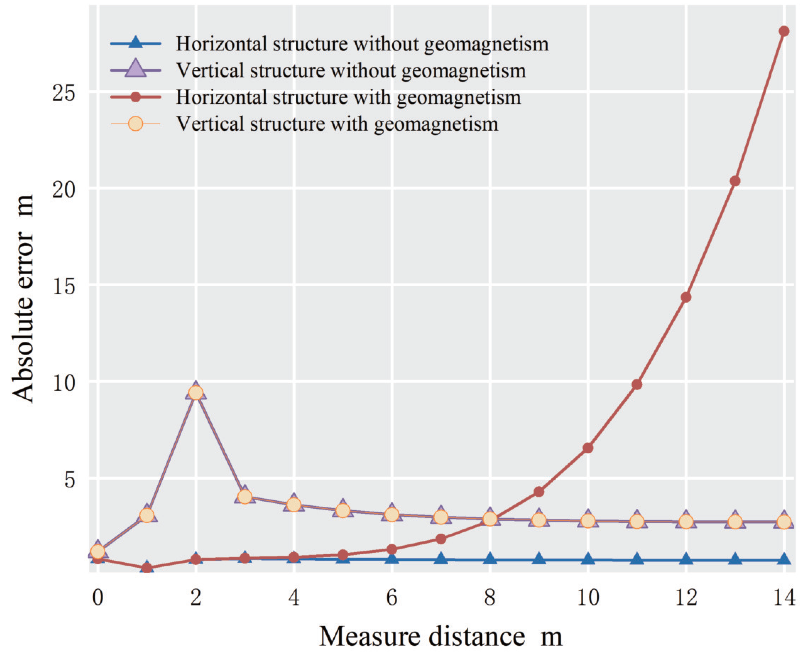
3.1.2. Comparison of Localization Accuracy between the Two Structures

The accuracy of the positioning was simulated experimentally by modeling the AUV’s movement in a fixed direction while locating a stationary target with its magnetic field generated by the magnetic dipole field model, as described in Table 3 for the simulation conditions. Due to the presence of some measurement errors in the actual background magnetic field, a 1% measurement error in the geomagnetic field was introduced during the simulation. The magnetic dipole was placed at (4, 5, 5), and the measurement system moved along the positive X-direction starting from (4, 5, 5).
The following Figure 5 illustrates a comparison of localization simulation results for the two structures. The abrupt error change at a distance of 2 m is due to the presence of specific field points around the magnetic dipole, causing the tensor matrix to become singular and resulting in the failure of the positioning method. In the absence of background magnetic field noise, both the horizontal and vertical structures demonstrate a favorable localization performance. When introducing 40,000 nT of magnetic field background noise, the horizontal structure experiences increasing positioning errors with the extension of the detection distance. In contrast, the vertical structure exhibits a superior positioning performance. Especially beyond the 8-m mark, the horizontal structure positioning method is significantly affected by the background magnetic field, and its performance deteriorates sharply. The vertical structure positioning algorithm described in this paper, on the other hand, does not directly utilize the measured magnetic field intensity data in the position vector calculation. Instead, it uses the data of its vertical differences. As a result, even in distant scenarios, it can still effectively extract the magnetic anomaly information generated by the magnetic anomaly. Therefore, it maintains good positioning accuracy in long-distance situations.

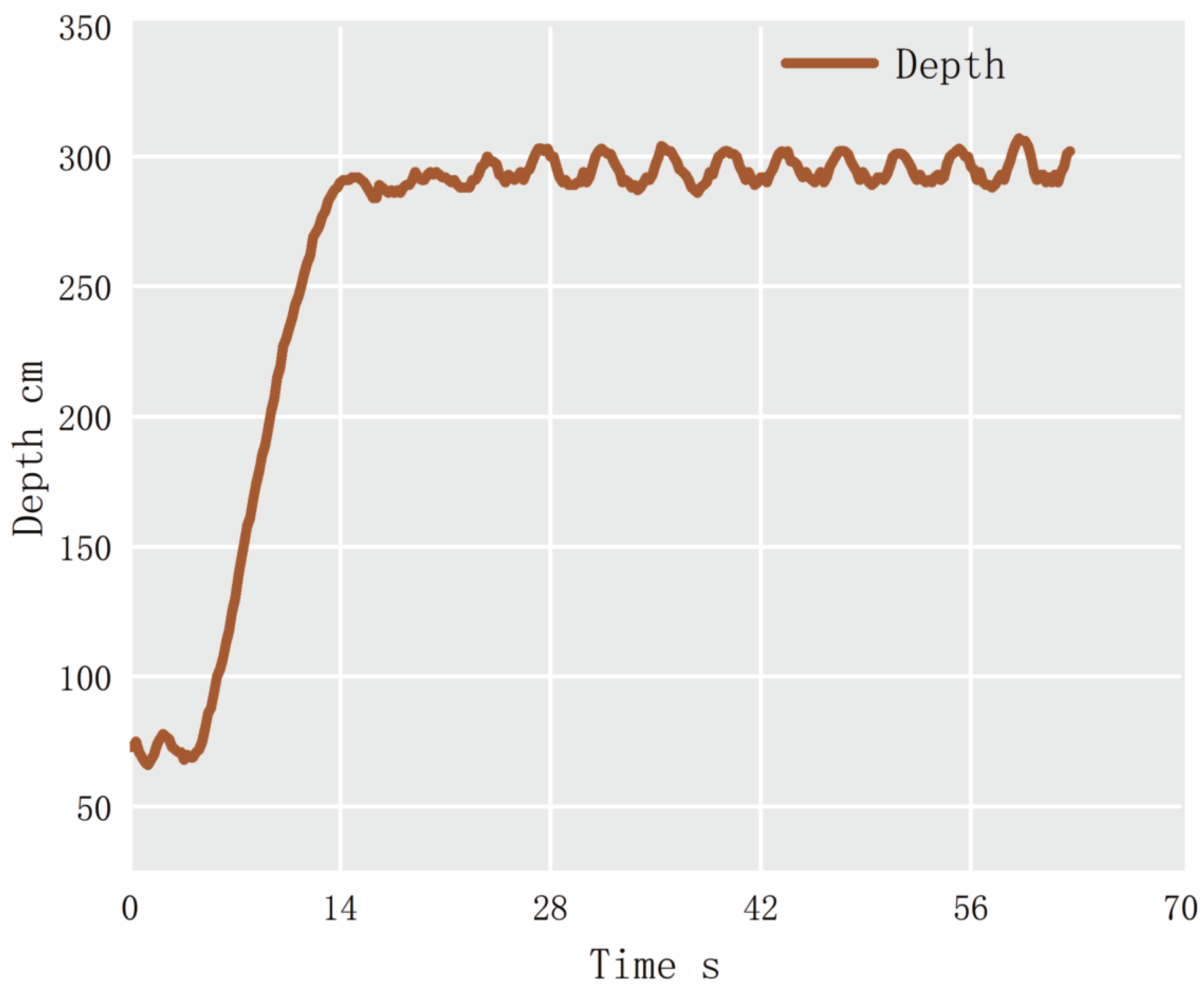
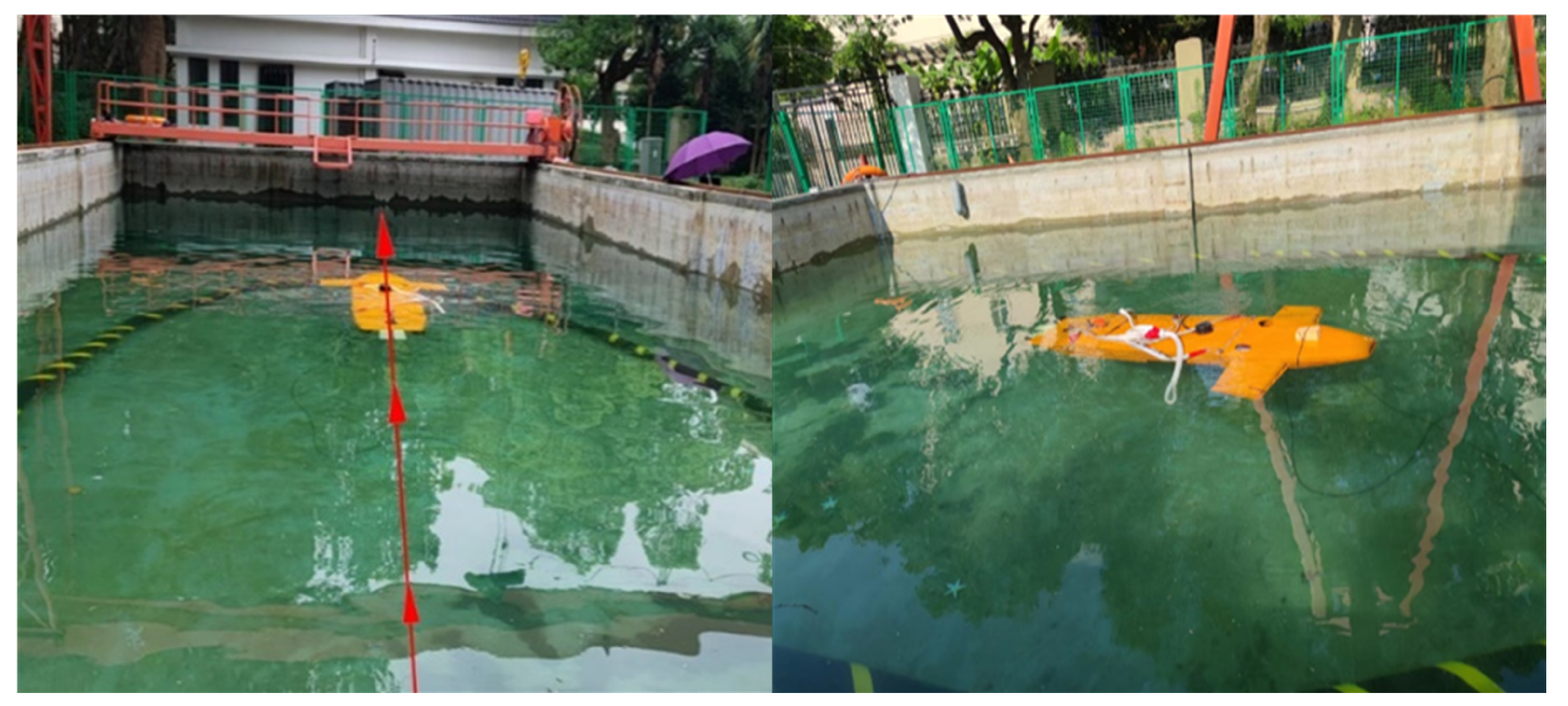
3.2. AUV Stability Experiment

To verify the excellent stability of the AUV, this paper conducted depth-keeping 3 m experiments. The actual depth was measured using a depth sensor, and the experiments were conducted in a specific nearshore area. The depth-keeping results are shown in the Figure 6.
According to Figure 6, it is evident that the AUV used in this study exhibits good stability. Therefore, using the AUV platform for magnetic anomaly localization is feasible. This implies that the AUV can provide sufficient stability when performing magnetic anomaly localization tasks, ensuring the accuracy and reliability of measurements. This is significant for magnetic anomaly research and localization.

3.3. Structural Experiment Comparison

3.3.1. Experimental Conditions

In this paper, three magnetic flux gate sensors are combined into a magnetic gradient array mounted on the AUV. The layout of the magnetic flux gate sensors is shown in Figure 1, with array baseline 1 measuring 1.2 m, array baseline 2 measuring 0.6 m, and the vertical baseline (i.e., the altitude difference) set at 1 meter. These sensors are arranged in an isosceles triangle configuration to achieve the measurement of the magnetic gradient tensor. The magnetic flux gate sensors exhibit excellent noise performance and sensitivity, with the main parameters listed in Table 4.
The provided information describes an experiment involving a magnetic target, which is the undersea cable as shown in Figure 7. The position information for the cable is (0 m, 15 m, 0 m), and the AUV starts from the initial point (0 m, 0 m, 0 m) and moves along the Y-axis at intervals of 1 m, performing both ascent and fixed-depth operations until it reaches the endpoint (0 m, 14 m, 0 m). During this movement, magnetic field data are collected using the magnetic gradient measurement array. The data collection duration is 60 s, with a sampling frequency of 0.75 Hz. A total of 15 sets of data are collected. The background magnetic field information for the experimental site is provided in Table 5:

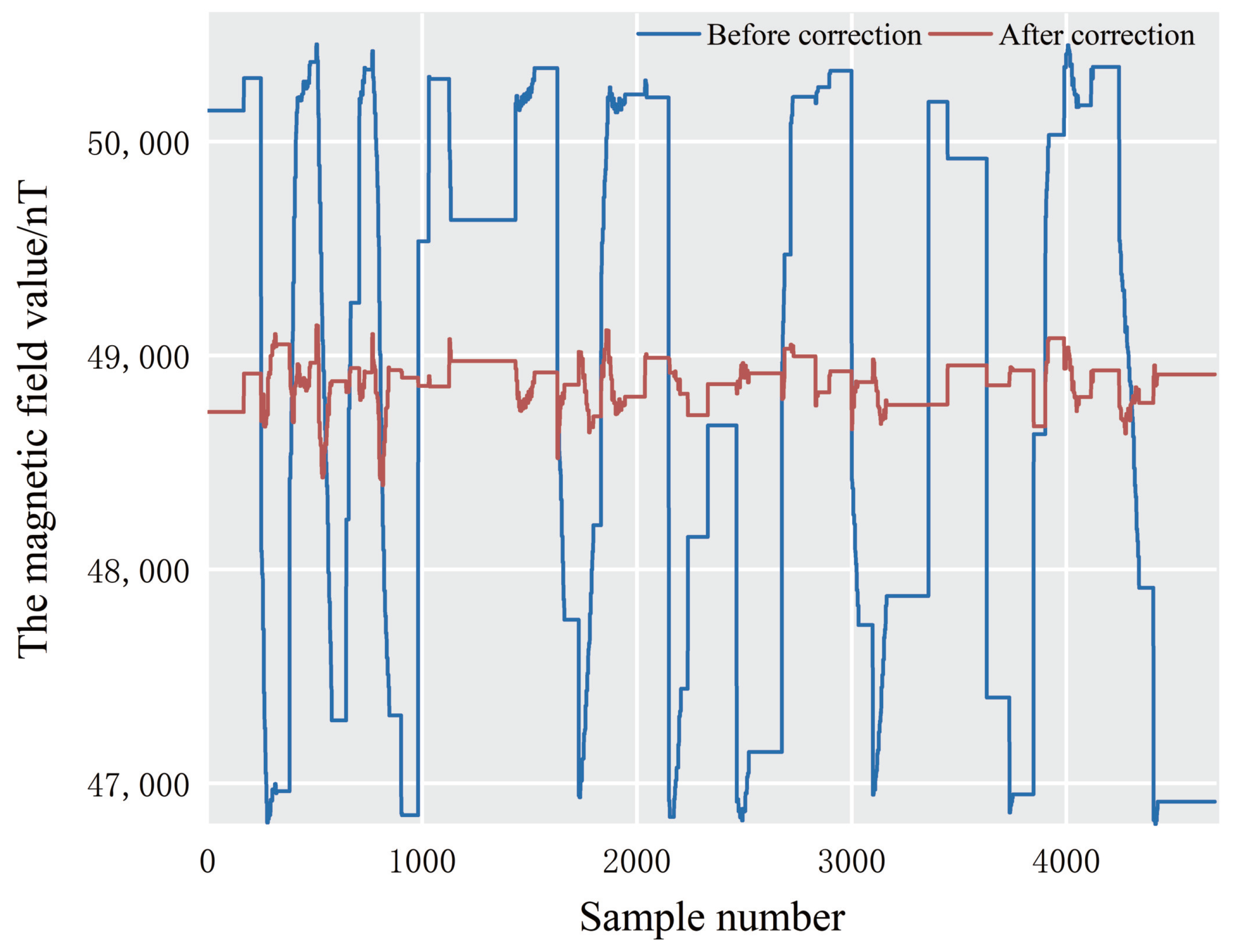
3.3.2. Analysis of Experimental Results

Due to the interference from the AUV’s own magnetic properties and time-varying noise during data collection, the measured data exhibit significant fluctuations [33,34]. The collected data are corrected using the Ocean Predator algorithm. In Figure 8, the gray line represents a set of experimental measurement data with a fluctuation range of 46.65 μ T to 50.48 μT and a variance of 1,791,836.522. The red line represents the magnetic field data after calibration using the Ocean Predator algorithm, with a fluctuation range of 48.45 μ T to 49.23 μ T and a variance of 10,894.87499. After calibration, gradient values are calculated to perform magnetic source localization.
After calibrating each set of data using the Ocean Predator algorithm, the average value of each set of data was computed to calculate the gradient values and perform magnetic source localization. The positioning error data is as shown in Table 6. The experimental results shown in Figure 9 indicate that, as the relative distance between the AUV and the underwater cable continuously increases, the localization errors of both structures and their positioning methods gradually increase with the experimental distance. In the near-field scenario (1 m to 5 m), the positioning accuracy of the two structures is quite close. The average positioning error for the horizontal structure is 1.504 m, while the average positioning error for the vertical structure is 1.476 m. In the far-field scenario (6 m to 15 m), due to the fact that in the positioning Formula (13) used for the horizontal structure, “B” actually refers to the magnetic field intensity generated by the magnetic anomaly source, not including the background field’s magnetic field intensity, the positioning accuracy of the vertical structure has consistently been superior to that of the horizontal structure. In this case, the magnetic field intensity generated by the magnetic anomaly source is already very weak in the far field and has become submerged within the background magnetic field.

4. Discussion

Based on the actual experiments, it has been observed that in the near field, the magnetic anomaly field of the target object does not become completely submerged within the background magnetic field. Traditional horizontal structure algorithms work well for positioning in the near field, but in the far field, the traditional horizontal structure positioning method cannot achieve accurate positioning for smaller-sized target objects. In subsequent simulation experiments, this paper adjusted the z-axis baseline, and the positioning error changed accordingly. When the Z-axis baseline was set to 0.5 m with the same geomagnetic field parameters as mentioned earlier, the far-field positioning error of the vertical positioning structure was much larger than that of the 1 m baseline distance. However, it is not advisable to have an excessively large vertical baseline in reality as it can affect the passage of the measuring vehicle. Due to experimental limitations, this paper did not verify the impact of changes in the Z-axis baseline on positioning errors. This is considered a potential area for future research. Furthermore, increasing the precision of the sensors can lead to a reduction in positioning errors with this algorithm. Additionally, from the simulation results of positioning accuracy, it can be observed that the algorithm exhibits a positioning error discontinuity at points where the magnetic gradient tensor matrix becomes singular. This should be actively avoided in practical applications. Therefore, one key focus of future research should be how to make the algorithm perform well at points where the magnetic gradient tensor matrix is singular.
In comparison to the vertical structure algorithm used in this paper, the current iterative positioning algorithms require relatively accurate initial values to achieve good results during iteration, and the algorithm’s time complexity is much higher than that of the algorithm used in this paper. Li’s algorithm, which is based on the eigenvalues and eigenvectors of the magnetic gradient tensor, requires prior knowledge of whether the observation system is above or below the magnetic target. It cannot uniquely solve for unknown large-scale positions or magnetic targets with vertical movement characteristics. In contrast, the algorithm in this paper does not require prior knowledge of the magnetic target’s direction and can compute a unique directional vector.
However, a limitation of this paper is that it uses a high-order and complex magnetic gradient tensor matrix, which imposes higher demands on sensor noise and errors. Additionally, compared to single-point positioning, the algorithm takes more time. At the same time, it is worth noting that AUVs are propelled by motors, and it is unavoidable that motor-generated magnetic fields are introduced during data collection. Firstly, it is essential to clarify that magnetic fields produced by underwater cables and ferromagnetic materials fall into the low-frequency range. Electric motors, however, can generate low-frequency 50 Hz magnetic fields and high-frequency magnetic fields based on 50 Hz harmonics. High-frequency magnetic fields can be filtered out using low-pass filters, while the low-frequency 50 Hz magnetic field can be mitigated by positioning magnetic sensors as far away from the propulsion system as possible. Therefore, if a magnetometer system is mounted on a drone platform, it is important to consider how to eliminate the influence of motor-generated magnetic fields.

5. Conclusions

This paper addresses underwater magnetic survey localization and accomplishes the following tasks:
  • A magnetic gradient tensor measurement device was designed and mounted on an AUV platform. Two magnetic gradient tensor measurement structures were implemented based on the AUV’s vertical ascent and descent capabilities. Comparative simulation experiments were conducted for these two structures;
  • Localization accuracy simulations were performed for the two magnetic gradient tensor structures and their corresponding positioning computation models;
  • Data collection was conducted using the AUV platform to analyze the localization performance of the two structures.
The simulation results and practical experimental results both indicate that, in the absence of geomagnetic background noise, the two methods and their positioning models yield consistent results. However, when subjected to the influence of geomagnetic background noise, the vertical structure exhibits superior long-distance positioning accuracy compared to the horizontal structure. Future work will consider further research into both structures when introducing AUV attitude errors and accounting for the impact of motor magnetic fields.

Author Contributions

Conceptualization, F.Z. and X.Z.; methodology, F.Z. and X.Z.; software, F.Z. and H.L.; validation, F.Z., X.Z. and H.L.; formal analysis, F.Z.; investigation, X.Z.; resources, X.Z.; datacuration, F.Z. and H.L. and S.Z.; writing—original draft preparation, F.Z.; writing—review and editing, F.Z. and Z.Z.; supervision, X.Z. and J.L.; project administration, X.Z. and J.L. All authors have read and agreed to the published version of the manuscript.

Funding

This research was funded by Key Research and Development Program of Zhejiang Province, grant number 2021C03013.

Institutional Review Board Statement

Not applicable.

Informed Consent Statement

Not applicable.

Data Availability Statement

Not applicable.

Conflicts of Interest

The authors declare no conflict of interest.

References

  1. Thum, G.W.; Tang, s.; Ahmad, S.A.; Alrifaey, M. Toward a Highly Accurate Classification of Underwater Cable Images via Deep Convolutional Neural Network. J. Mar. Sci. Eng. 2020, 8, 924. [Google Scholar] [CrossRef]
  2. Glaviano, F.; Esposito, R.; Cosmo, A.D.; Esposito, F. Management and Sustainable Exploitation of Marine Environments through Smart Monitoring and Automation. J. Mar. Sci. Eng. 2022, 10, 297. [Google Scholar] [CrossRef]
  3. Chen, L.; Yang, Y.; Wang, Z.; Zhang, J.; Zhou, S.; Wu, L. Underwater Target Detection Lightweight Algorithm Based on Multi-Scale Feature Fusion. J. Mar. Sci. Eng. 2023, 11, 320. [Google Scholar] [CrossRef]
  4. Luna, V.; Silva, R.; Mendoza, E.; Canales-García, I. Recording the Magnetic Field Produced by an Undersea Energy Generating Device: A Low-Cost Alternative. J. Mar. Sci. Eng. 2023, 11, 1423. [Google Scholar] [CrossRef]
  5. Pei, Y.H.; Yeo, H.G.; Kang, X.Y. Magnetic gradiometer on an AUV for buried object detection. In Proceedings of the OCEANS 2010 MTS/IEEE, Seattle, WA, USA, 20–23 September 2010. [Google Scholar]
  6. Kasaya, T.; Nogi, Y.; Kitada, K. Advanced magnetic survey system and method for detailed magnetic field mapping near the sea bottom using an autonomous underwater vehicle. Explor. Geophys. 2023, 54, 205–216. [Google Scholar] [CrossRef]
  7. Liang, K.; Xie, H.; Wang, G. Multiple Underwater Magnetic Targets Location Method Based on Neural Network. In Proceedings of the 2021 4th International Conference on Advanced Electronic Materials, Computers and Software Engineering (AEMCSE), Changsha, China, 26–28 March 2021. [Google Scholar]
  8. Chen, L.; Feng, Y.; Wu, P.; Zhu, W.; Fang, G. An Innovative Magnetic Anomaly Detection Algorithm Based on Signal Modulation. IEEE Trans. Magn. 2020, 56, 6200609. [Google Scholar] [CrossRef]
  9. Yu, H.; Bo-Wen, W.; Li-Hua, W. An Innovative heoretical Investigation on the Linear Location Algorithm of the Magnetic Gradient Tensor Ranging by Use of Cuboid Triaxial Magnetometer Array. IEEE Trans. Magn. 2021, 57, 99. [Google Scholar] [CrossRef]
  10. Zhou, J.; Wang, C.; Peng, G.; Yan, H.; Zhang, Z.; Chen, Y. Magnetic anomaly detection via a combination approach of minimum entropy and gradient orthogonal functions. ISA Trans. 2023, 134, 548–560. [Google Scholar] [CrossRef]
  11. Wynn, W.; Frahm, C.; Carroll, P.; Clark, R.; Wellhoner, J.; Wynn, M. Advanced superconducting gradiometer/Magnetometer arrays and a novel signal processing technique. IEEE Trans. Magn. 1975, 11, 701–707. [Google Scholar] [CrossRef]
  12. Sui, Y.; Leslie, K.; Clark, D. Multiple-Order Magnetic Gradient Tensors for Localization of a Magnetic Dipole. IEEE Magn. Lett. 2017, 8, 6506605. [Google Scholar] [CrossRef]
  13. Jin, H.; Guo, J.; Wang, H.; Zhuang, Z.; Qin, J.; Wang, T. Magnetic Anomaly Detection and Localization Using Orthogonal Basis of Magnetic Tensor Contraction. IEEE Trans. Geosci. Remote Sens. 2020, 58, 5944–5954. [Google Scholar] [CrossRef]
  14. Li, Q.; Shi, Z.; Li, Z.; Fan, H.; Zhang, G.; Li, T. Magnetic Object Positioning Based on Second-Order Magnetic Gradient Tensor System. IEEE Sens. J. 2021, 21, 18237–18248. [Google Scholar] [CrossRef]
  15. Deng, H.; Hu, X.; Cai, H.; Liu, S.; Peng, R.; Liu, Y.; Han, B. 3D Inversion of Magnetic Gradient Tensor Data Based on Convolutional Neural Networks. Minerals 2022, 12, 566. [Google Scholar] [CrossRef]
  16. Li, Q.; Li, Z.; Shi, Z.; Fan, H. Application of Helbig integrals to magnetic gradient tensor multi-target detection. Measurement 2022, 200, 111612. [Google Scholar] [CrossRef]
  17. Nara, T.; Suzuki, S.; Ando, S. A Closed-Form Formula for Magnetic Dipole Localization by Measurement of Its Magnetic Field and Spatial Gradients. IEEE Trans. Magn. 2006, 42, 3291–3293. [Google Scholar] [CrossRef]
  18. Wang, S.; Zhang, M.; Zhang, N.; Guo, Q. Particle Swarm Optimization with Rotation Axis Fitting for Magnetometer Calibration. J. Syst. Eng. Electron. 2018, 29, 456–461. [Google Scholar]
  19. Wiegert, R.F.; Purpura, J.W. Magnetic Scalar Triangulation and Ranging system for autonomous underwater vehicle based detection, localization and classification of magnetic mines. In Proceedings of the Oceans ’04 MTS/IEEE Techno-Ocean, Kobe, Japan, 9–12 November 2004. [Google Scholar]
  20. Iacca, G.; Bakker, F.L.; Wörtche, H. Real-time magnetic dipole detection with single particle optimization. Appl. Soft Comput. Appl. Soft Comput. 2014, 23, 460–473. [Google Scholar] [CrossRef]
  21. Yin, G.; Li, P.; Wei, Z.; Liu, G.; Yang, Z.; Zhao, L. Magnetic dipole localization and magnetic moment estimation method based on normalized source strength. J. Magn. Magn. Mater. 2020, 502, 166450. [Google Scholar] [CrossRef]
  22. Wang, M.; Song, S.; Liu, J.; Meng, M.Q.H. Multipoint Simultaneous Tracking of Wireless Capsule Endoscope Using Magnetic Sensor Array. IEEE Trans. Instrum. Meas. 2021, 70, 1–10. [Google Scholar] [CrossRef]
  23. Yang, W.; Li, Y.; Hu, C.; Song, S. A real-time tracking method for the rectangular magnet based on parallel Levenberg-Marquardt algorithm. Int. J. Appl. Electromagn. Mech. 2011, 37, 241–251. [Google Scholar] [CrossRef]
  24. Liu, H.; Wang, X.; Zhao, C.; Ge, J.; Dong, H.; Liu, Z. Magnetic Dipole Two-Point Tensor Positioning Based on Magnetic Moment Constraints. IEEE Trans. Instrum. Meas. 2021, 70, 9700410. [Google Scholar] [CrossRef]
  25. Li, Q.; Shi, Z.; Li, Z.; Mu, L.; Fan, H. Magnetic object positioning method based on tensor spacial invariant relations. Meas. Sci. Technol. 2020, 31, 115015. [Google Scholar] [CrossRef]
  26. Yuz, H.T.; Lv, J.W.; Fan, L.H.; Zhang, B.T. An improved method of target location based on magnetic gradient tensor. Syst. Eng. Electron. Technol. 2014, 36, 1250–1254. (In Chinese) [Google Scholar]
  27. Jiang, B.; Xu, Z.; Yang, S.; Chen, Y.; Ren, Q. Profile Autonomous Underwater Vehicle System for Offshore Surveys. Sensors 2023, 36, 3722. [Google Scholar] [CrossRef] [PubMed]
  28. Allen, G.I.; Sulzberger, G.; Bono, J.T.; Pray, J.S.; Clem, T.R. Initial Evaluation of the New Real-time Tracking Gradiometer Designed for Small Unmanned Underwater Vehicles. In Proceedings of the OCEANS 2005 MTS/IEEE, Washington, DC, USA, 17–23 September 2005. [Google Scholar]
  29. Allen, G.I.; Matthews, R.; Wynn, M. Mitigation of Platform Generated Magnetic Noise Impressed on a Magnetic Sensor Mounted in an Autonomous. Underwater Vehicle. In Proceedings of the MTS/IEEE Oceans, Honolulu, HI, USA, 5–8 November 2001. [Google Scholar]
  30. Pei, Y.H.; Yeo, H.G. UXO survey using vector magnetic gradiometer on autonomous underwater vehicle. In Proceedings of the OCEANS ‘09 MTS/IEEE, Biloxi, MS, USA, 26–29 October 2009. [Google Scholar]
  31. Kumar, S.; Perry, A.R.; Moeller, C.R.; Skvoretz, D.C. Real-time tracking magnetic gradiometer for underwater mine detection. In Proceedings of the Oceans ’04 MTS/IEEE, Kobe, Japan, 9–12 November 2004. [Google Scholar]
  32. Wang, S.; Zhang, M.; Zhang, N.; Guo, Q. Calculation and correction of magnetic object positioning error caused by magnetic field gradient tensor measurement. J. Syst. Eng. Electron. 2018, 29, 456–461. [Google Scholar]
  33. Faramarzi, A.; Heidarinejad, M.; Mirjalili, S.; Gandomi, S. CMarine Predators Algorithm: A nature-inspired metaheuristic. Expert Syst. Appl. 2020, 152, 113377. [Google Scholar] [CrossRef]
  34. Riwanto, B.A.; Tikka, T.; Kestilä, A.; Praks, J. Particle Swarm Optimization with Rotation Axis Fitting for Magnetometer Calibration. IEEE Trans. Aerosp. Electron. Syst. 2017, 53, 1009–1022. [Google Scholar] [CrossRef]
Figure 1. Horizontal magnetic gradient tensor structure.
Jmse 11 01909 g001
Figure 2. Vertical gradient tensor structure.
Jmse 11 01909 g002
Figure 3. Flowchart of the Vertical Magnetic Gradient Structural Algorithm.
Jmse 11 01909 g003
Figure 4. Comparison of the components of two magnetic gradient structures. (a) compares B x x solved for two magnetic gradient structures with theoretical values. (b) compares B x y solved for two magnetic gradient structures with theoretical values. (c) compares B x z solved for two magnetic gradient structures with theoretical values. (d) compares B y y solved for two magnetic gradient structures with theoretical values. (e) compares B y z solved for two magnetic gradient structures with theoretical values.
Jmse 11 01909 g004
Figure 5. Positioning accuracy of horizontal and vertical structures with and without geomagnetic field noise.
Jmse 11 01909 g005
Figure 6. AUV at 3 m depth result.
Jmse 11 01909 g006
Figure 7. Motion path of AUV acquisition data.
Jmse 11 01909 g007
Figure 8. Comparison of data before and after TMI calibration.
Jmse 11 01909 g008
Figure 9. Comparison of positioning accuracy between horizontal and vertical structures.
Jmse 11 01909 g009
Table 1. Different structure magnetic gradient tensor simulation conditions.
Parameter NameParameter
Array baseline 11.2 m
Array baseline 20.6 m
Vertical Baseline1 m
Magnetic Moment3000 A·m
Magnetic Inclination60°
Magnetic declination
Table 2. Component R M S E values of two magnetic gradient structures.
B xx B xy B xz B yy B yz
Horizontal Structure4.610218.386814.147615.743518.8295
Vertical Structure4.610218.38686.397315.74359.8696
Table 3. Positioning accuracy simulation conditions.
Parameter NameParameter
Array baseline 11.2 m
Array baseline 20.6 m
Vertical Baseline1 m
Background Magnetic Field40,000 nT
Magnetic Moment3000 A·m
Magnetic Inclination60°
magnetic declination
Table 4. Fluxgate sensor parameters.
Parameter NameParameter
Measurement Range−100 μ T +100 μ T
Resolution0.1 nT
Bandwidth0.5 dB
Linearity<0.01% FS
Noise Level<1 nT.RMS @0.1 s
Table 5. Background magnetic field information of test site.
TMIMag_DeclinationMag_Inclination
48,820.3 nt−5°57′46°1′
Table 6. Positioning error of horizontal structure and vertical structure.
Distance (m)Horizontal Structural ErrorVertical Structural Error
10.440.68
21.401.94
31.181.38
41.820.63
52.682.75
64.482.97
74.432.22
85.472.56
96.423.34
107.475.17
118.435.89
129.327.03
139.854.49
1411.317.43
1512.335.42
Disclaimer/Publisher’s Note: The statements, opinions and data contained in all publications are solely those of the individual author(s) and contributor(s) and not of MDPI and/or the editor(s). MDPI and/or the editor(s) disclaim responsibility for any injury to people or property resulting from any ideas, methods, instructions or products referred to in the content.

