Analysis of Water Hammer and Pipeline Vibration Characteristics of Submarine Local Hydraulic System

Abstract

The hydraulic pipeline vibration noise is one of the main noise sources in submarine stealth conditions. Taking the local hydraulic system of a certain type of submarine as the research object, a model is first developed to simulate water hammer pressures and to study the influence of component parameters on the generation and transmission of water hammers. Then, using the maximum water hammer as the excitation, fluid–structure interaction (FSI) vibration characteristics analysis of the pipeline is carried out. Additionally, the simulation method of clamp bolt pre-tightening is discussed. Finally, the modal test of various specifications of the pipeline is carried out. The results show that the error between the simulation and the test results is within 10%, which verifies the correctness of the model settings. On this basis, with the position of the clamp as the independent variable and the maximum stress of pipelines as the dependent variable, the optimization of pipeline passive vibration control is carried out by genetic algorithm, and the finite element verification shows that the pipeline vibration stress is effectively reduced.

1. Introduction

Hydraulic pipelines, as power and energy transmission channels for large, heavy equipment, are known as the “blood vessels” of the hydraulic system [1]. With the advancement of China’s maritime power strategy, the submarine hydraulic system is developing in the direction of high speed and high pressure. Taking a newly developed submarine as an example, its hydraulic system is gradually upgraded from the commonly used 10 MPa pressure system to the 16 MPa pressure system. This transition brings vibration and noise problems that not only reduce the reliability of the pipeline itself but also have a more significant negative impact on the acoustic hidden characteristics. Therefore, developing and applying submarine acoustic stealth technology has become a key technical means to enhance submarine survivability.

The pressure impact caused by load changes, as well as the water hammer effect caused by the opening and closing of control valves, can generate significant vibration and noise in the pipeline [2]. The ‘pipeline–clamp’ system is the main transmission path of submarine hydraulic pipeline vibration. The clamp transfers the vibration energy to the hull, resulting in unfavorable factors for stealth. Therefore, the vibration problems caused by the water hammer in the submarine hydraulic pipeline cannot be ignored. In previous studies, pipelines and clamps were usually separated for research, and clamps have been improved from the traditional all-metal components to rubber clamps, elastic components, etc., so it is necessary to carry out pipeline vibration research in the new situation.

Domestic and foreign scholars have carried out many studies on water hammers through model numerical calculation and experimental methods. Pal S [3] demonstrates that the first-order Godunov’s scheme compares favorably with the method of characteristics (MOC) in terms of accuracy and computational speed through numerical and experimental studies. With further advances in finite volume method (FVM) schemes, it can achieve faster and more accurate codes. Zhang [4] conducted research on the valve closure law under four flow characteristics based on an unsteady friction model and obtained the relationship between the valve control rate and the peak value of the water hammer. Liu [5,6] used a genetic algorithm to optimize the valve closure law for controlling the maximum peak pressure of the water hammer and trained a specific system valve closure law prediction model through the radial neural network based on a large amount of data. Chen [7] studied the dynamic structure interaction responses to water hammer in a reservoir–pipe–valve physical system and discussed hydraulic pressure, pipe wall stress, and axial motion concerning different parameters. Afshar [8] proposed an implicit method of characteristics to solve problems of transient flow caused by the closure of a valve and failure of a pump system, which alleviates the shortcomings and limitations of the most commonly used conventional MOC.

At present, a lot of research work has been carried out in fluid–structure interaction (FSI) vibration modeling, construction of clamp models, and finite element analysis of pipelines. Mikota obtained the frequency response function of the pipeline by applying the fluid excitation load and analyzed the mechanical properties of the pipeline system to obtain the natural frequency, relative vibration mode, and other mechanical properties of the pipeline system [9,10]. Hosseini [11] simulated various types of viscoelastic supports and investigated their effects on the FSI during the water hammer in straight pipeline systems. Ulanov [12,13] used ANSYS to model the pipeline and clamp, calculate the stiffness, damping, and other parameters of the clamp, and obtain the vibration response of the pipeline under the constraint of the clamp through harmonic response analysis. Chai [14,15,16] established the clamp-straight pipe dynamics model based on the six-degree-of-freedom beam element. By solving the stiffness of the double-clamp, the dynamic model of a pipeline system with a single double-clamp was established, and the influence of the clamp installation torque on the natural frequency of the pipeline was studied. However, existing analyses mostly focus on FSI mathematical models or other fields, and it is relatively rare to conduct vibration research on submarine hydraulic pipeline systems considering FSI effects.

The ultimate goal of pipeline FSI research is to reduce pipeline vibration and pipeline failure events caused by FSI. In addition to system vibration control from the perspective of fluid control, passive, active, semi-active, and hybrid control of pipeline vibration have been developed from the pipeline itself or other auxiliary equipment. Among them, the passive vibration control of the pipeline does not require external power and only relies on the vibration energy and constraints of the pipeline itself to control the vibration. Commonly used methods include installing elastic clamps, optimizing the position of the clamps, and installing dynamic vibration absorbers [17,18]. Liu analyzed the stiffness and damping characteristics of aviation pipeline clamps, gave a clear method for measuring the equivalent stiffness and damping of clamps, and studied the impact of stiffness and damping changes on pipeline vibration [19]. For vibration analysis and control of the multi-pump system, Li proposed to apply the Chaotic Swarm Particle Optimization (CPSO) algorithm to optimize the clamps’ position, and the minimum objective function decreased by 36.4% compared to the value of the original clamps’ locations [20]. Quan used sensitivity analysis and a genetic algorithm to sort the contribution of variables and optimize the support layout of multivariable pipeline systems, achieving a good vibration control effect [21]. The dynamic vibration absorber was initially proposed by Frahm [22]. After that, many scholars conducted research on the effect of introducing nonlinear damping into the dynamic vibration absorber. For example, Jiang [23] analyzed the vibration and noise caused by the onboard pipeline system and proposed a new concept, “pressure-stabilized bladder,” to reduce the vibration and noise caused by the pipeline system. Song [24] proposed the pounding tuned mass damper to mitigate the vibration of the flexible pipeline structures and verified its vibration control performance through numerical analysis and experimental research.

The structure of the paper is as follows: Firstly, the flow and pressure characteristics analysis model of the hydraulic system is established, and the influence of the reversing time on the valve-closed water hammer is studied. Afterward, the model of the pipeline–clamp system is established, and the natural frequency and response modes of the pipeline structure are obtained by modal analysis and test under the conditions of liquid filling and clamps constraint. Compared with the hammer test, the correctness of the model and simulation analysis method is verified. In the next part, taking the maximum valve-closure water hammer as the excitation, the simplified FSI analysis method is used to analyze the vibration of the pipelines in various regions. Finally, a genetic algorithm is used to optimize the passive vibration control of typical pipeline units and explore vibration control methods for submarine hydraulic pipelines.

2. Principle of Local Hydraulic System and Construction of AMESim Model

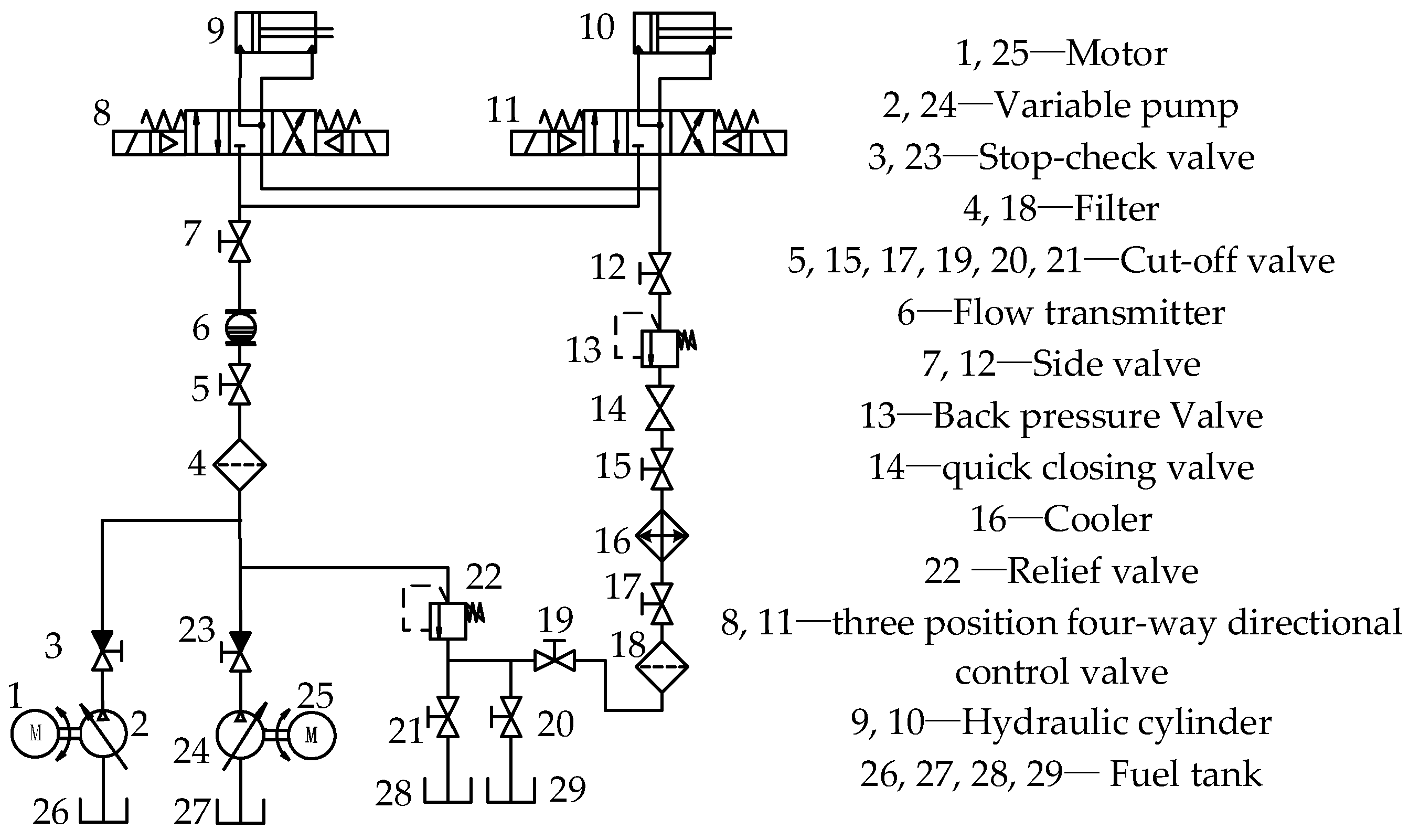
2.1. Principle of Local Hydraulic System

The schematic diagram of the local hydraulic system of a submarine is shown in Figure 1. The pressure is provided by two sets of hydraulic pump sources. Two three-position, four-way directional valves control two sets of hydraulic cylinders, respectively, which are the main action components that cause water hammer. The hydraulic cylinder is placed vertically with the load. Fast-closing valves, cut-off valves, etc. are used for safety protection. Hydraulic accessories such as filters and coolers are used to ensure oil cleaning and maintain system temperature.

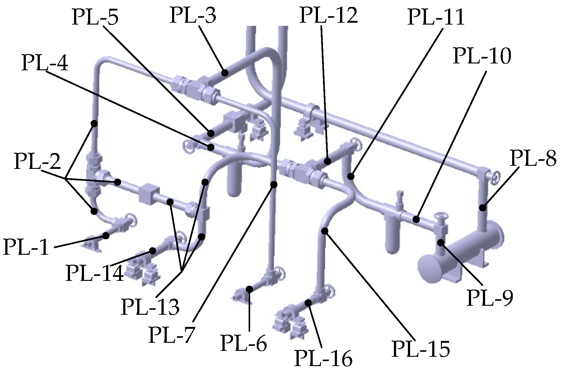
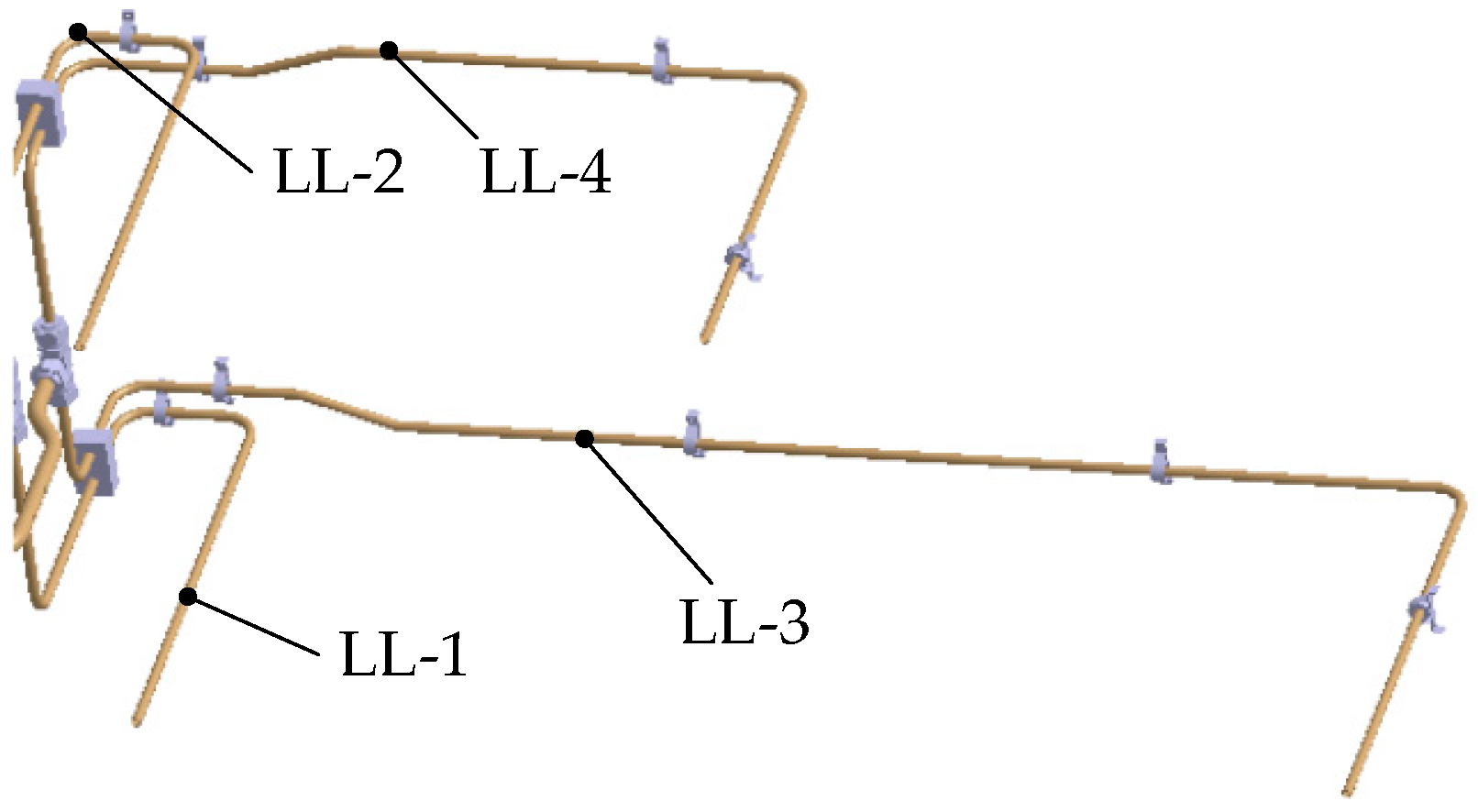
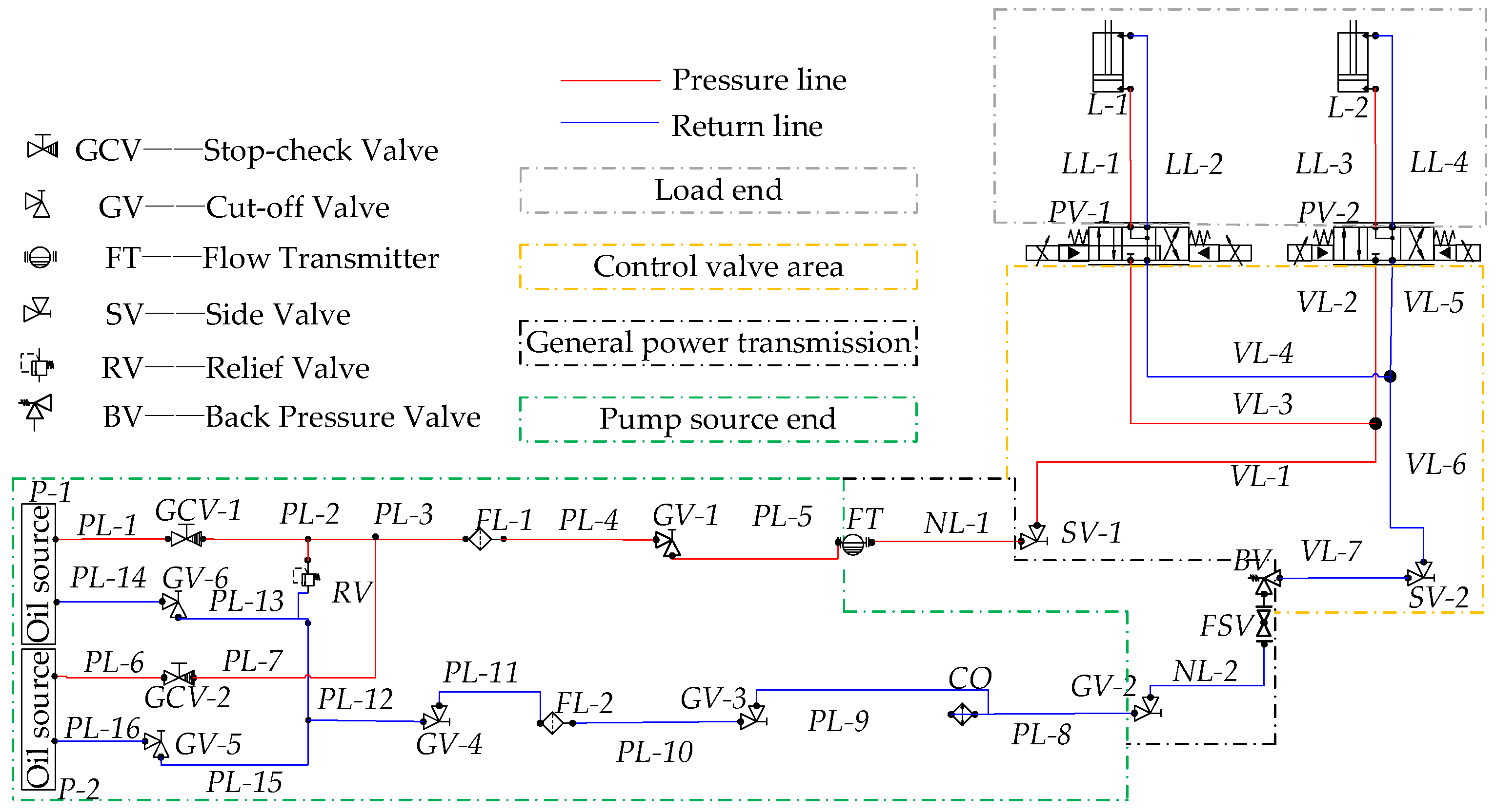
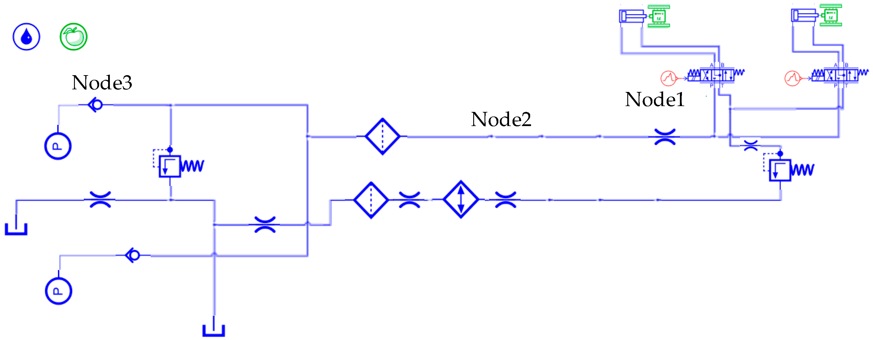
2.2. Topological Structure Division of Hydraulic Pipeline System

There are many branches in the pipelines of the local hydraulic system. The local hydraulic system is divided into four pipeline subsystems: pump source end, general power transmission, control valve area, and load end. This facilitates identifying the results of the pressure calculation of the corresponding pipelines, combined with the working principle of the local hydraulic system and pipeline excitation (pump port flow and pressure pulsation, water hammer caused by valve opening and closing, and load changes). All four subsystems include pressure and return lines. The partitioning results are shown in Figure 2.

2.3. AMESim Modeling of Local Hydraulic System

Two sets of oil sources are backed up to each other, and their parameters are shown in

Table 1. Oil Source Parameters.

Parameter Name	Value	Unit	Parameter Name	Value
rated pressure	16	MPa	rated speed r	1400 r/min
installed power	≤14	kW	outlet flow q	0–40 L/min

. The three-position, four-way directional valve is controlled by the reversing electrical signal source, which is set in three stages. The meaning of each stage is shown in

Table 2. Segmented control of Commutation electrical signal.

Phase	Time (s)	Purpose
1	0–3	system pressure reaches 16 MPa
2	3–3.03	directional valve switching, p port closed
3	3.03–6.03	p port keeps closed

.

The number of pipelines is large, and their internal flow and pressure fluctuation are the main factors to be considered in the FSI dynamics calculation. Therefore, we not only need to consider the capacitance (C) and resistance (R) of the pipeline but also its inertia (I). Capacitance mainly affects pressure calculation, resistance affects pressure loss along the way, and inertia affects the calculation of the fluctuation effect. In the specific calculation, the more detailed the pipeline model, the closer it is to the actual situation, and the calculation time also increases. In the specific calculation, the more detailed the pipeline model, the closer it is to the actual situation, but the calculation time also increases accordingly. Therefore, the pipeline sub-model is selected based on its specific location. The HL0040 pipeline sub-model is used in the front pipelines of the electromagnetic directional valve due to a strong water hammer caused by valve closure. The general power transmission pipelines have a large aspect ratio, and the pressure drop during oil transmission cannot be ignored. Therefore, the HL0010 pipeline sub-model is selected. The length of the remaining pipeline units is short, and the internal transmission of oil is not complicated. Therefore, the HL0001 pipeline sub-model is selected. The final flow and pressure calculation model of the local hydraulic system is shown in Figure 3.

3. Analysis of Water Hammer Transmission and Influence Law

3.1. Empirical Formula for Calculating Water Hammer Wave Pressure and Wave Velocity

When changing the direction of the valve, the sudden opening and closing of the valve port will generate a short and obvious water hammer effect at the valve port. The flow rate of hydraulic oil in the pipeline will change suddenly, converting liquid power energy into pressure energy in a very short period and generating water hammer waves in the pipeline. The transmission velocity of the water hammer wave is [23,24,25]:

$$a=\frac{1}{\sqrt{\rho \left(\frac{1}{K}+\frac{D}{Ee}\right)}}$$

(1)

where K is the bulk modulus of fluid, E is the elastic modulus of pipeline material, e is the wall thickness of the pipeline, and D is the inner diameter of the pipeline.

According to the law of conservation of momentum, $mv=\Delta pAt$, the pressure impact is:

ΔP × A = ρAac

(2)

where ΔP is the pressure increment generated by the water hammer, A is the cross-sectional area of the pipeline. ρ is the density of the fluid, a is the propagation velocity of the water hammer wave in the pipeline, and c is the fluid velocity.

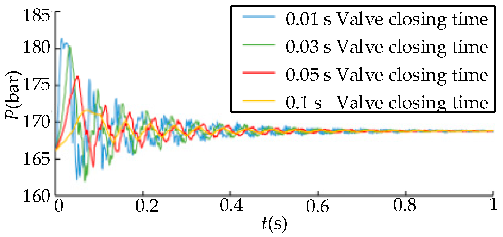
3.2. Analysis of the Influence of Valve Closing Time on Water Hammer

The closing time of the two directional valves in the system is taken as a variable to analyze the influence on the peak value and fluctuation time of the valve closing water hammer. The valve closing time is set to 0.01 s, 0.03 s, 0.05 s, and 0.1 s, respectively.

The pressure is observed at node 1 (in front of the valve), node 2 (the general long straight section), and node 3 (near the pump source) in Figure 3. At different closing times, the water hammer wave curve of node 1 is shown in Figure 4.

The overall analysis shows that the shorter the closing time of the valve, the more violent the pressure fluctuations in the hydraulic pipeline, the longer the fluctuation duration, the shorter the fluctuation period is (T_0.01 = 0.078 s, T_0.03 = 0.097 s, T_0.05 = 0.114 s, T_0.1 = 0.162 s), and the slower the attenuation. Moreover, as the valve closing time increases, the time when the pressure peak appears is relatively delayed, and the rate of pressure increase decreases. After the valve is closed, the water hammer pressure finally stabilizes at about 168.8 bar, which is about 2 bar higher than the normal working pressure. The simulation analysis shows that the larger the valve closing time, the smaller the water hammer fluctuation. However, the conclusion is no longer applicable when the valve closing time is large to a certain extent, and increasing the valve closing time will not infinitely suppress the water hammer effect. When the time is set to about 2 s, the pressure of the water hammer wave is stable near 168.8 bar, and there are no fluctuations. The result is shown in Figure 5.

For a certain system, when the valve closing time increases to a certain value, its impact on the pressure fluctuation of the system’s water hammer diminishes, and the water hammer effect no longer shows obvious oscillation attenuation characteristics. The pressure rises gently to the steady-state pressure, but the rapidity of system control decreases.

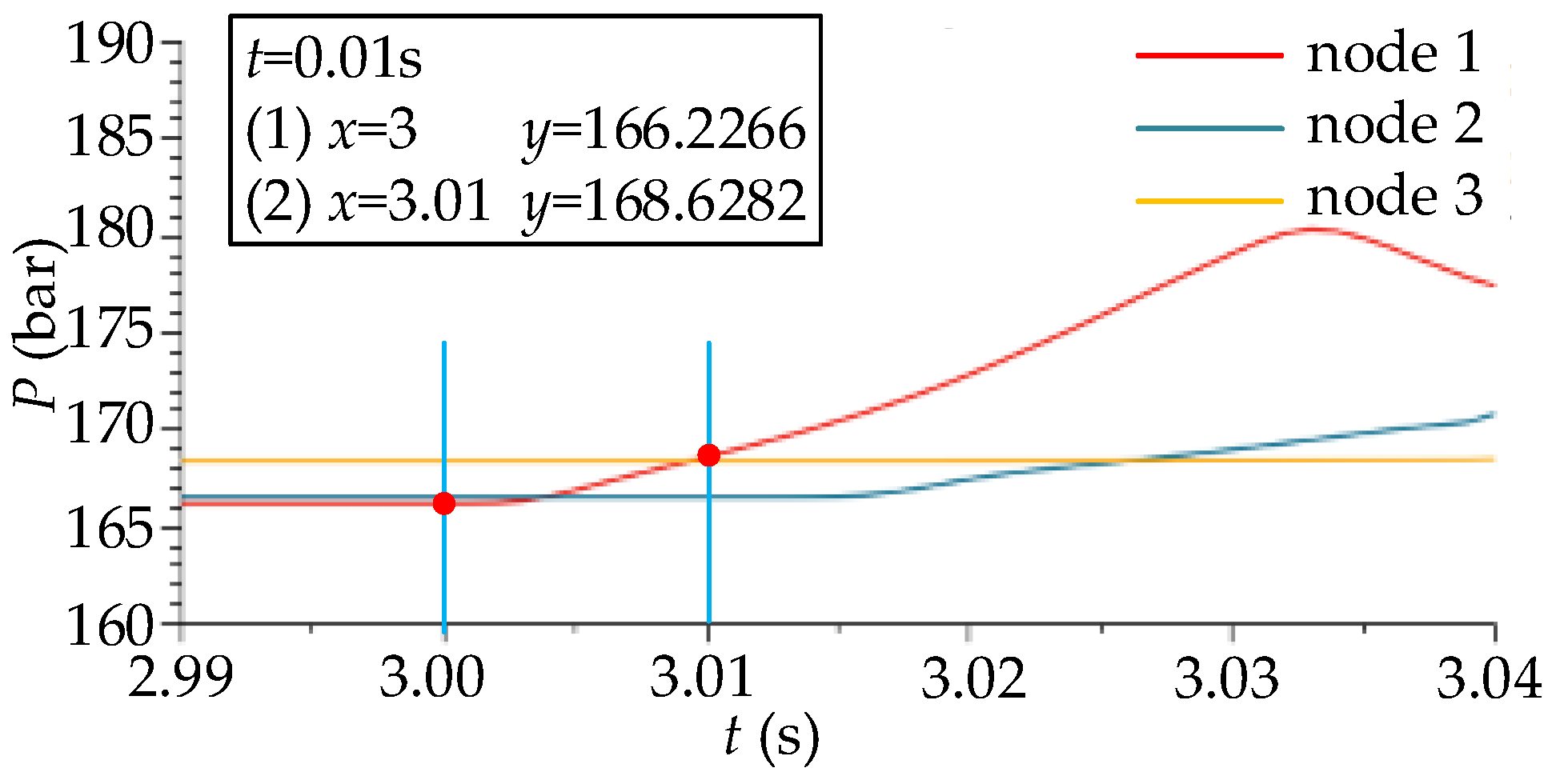
3.3. Analysis of the Transmission and Attenuation Characteristics of the Valve-Closing Water Hammer

Comparing the pressure fluctuation curves of the three nodes under each valve closing time, the results are shown in Figure 6. The peak of the water hammer wave pressure of the three nodes at each valve closing time is shown in

Table 3. Statistics of the peak pressure of a three-node water hammer at different valve closing times.

Valve Closing Time (s)	Node 1 (bar)	Node 2 (bar)	Node 3 (bar)
0.01	181.35	176.46	174.63
0.03	180.35	173.93	172.37
0.05	176.22	171.23	168.84
0.1	171.65	169.67	168.68

.

From the overall results, on the one hand, the water hammer wave has a certain time lag (manifested as the increase in pressure and the lag of peak time) when transmitting from the valve end to the pump source end. This feature shows the transmission characteristics of the water hammer wave, i.e., when it is transmitted from the valve end to the pump source end, the peak pressure appears at different times, which is related to the propagation velocity of the water hammer wave and the length of the pipeline. On the other hand, at each measuring point, the water hammer wave shows the characteristics of waveform oscillation and amplitude attenuation. The closer to the position of the valve, the more obvious the oscillation and the greater the amplitude.

The water hammer fluctuation curves of three nodes at 0.01 s valve closing time are locally enlarged, as shown in Figure 7.

It can be seen that before the valve is fully closed (3–3.01 s), the fluid pressure at nodes 2 and 3 is basically stable. In addition, the steady flow direction is positive from node 3 to node 1, and the steady-state pressure shows a trend of node 3 > node 2 > node 1. After the water hammer is generated, the water hammer wave is transmitted in a positive direction from node 1 to node 3. The peak value of the water hammer wave shows a trend of node 1 > node 2 > node 3, mainly caused by frictional head loss and local head loss in the fluid flow process. The steady-state pressure, the peak value of water hammer wave pressure, and the degree of fluctuation decrease along the forward flow direction. The water hammer wave near the pump source end is more stable, mainly because there is a stop check valve and a relief valve at the pump source end. The stop-check valve makes the oil only flow into the pipeline from the high-pressure oil of the pump source, so the water hammer wave cannot be affected by the rigid wall (the fluid is a viscoelastic medium), and the relief valve plays a good role in overflow. In the process of closing the valve (3–3.01 s), the opening and flow area of the directional valve gradually decrease, resulting in a decrease in fluid flow, which makes the system pressure increase. When the directional valve is completely closed, the system pressure gradually reaches its maximum value, and the maximum value occurs in a period after the valve is closed, which is mainly caused by the continuous supplementation and compression of subsequent fluids.

4. Vibration Characteristics Analysis of the Submarine Hydraulic Pipeline System

The hydraulic control system of the submarine adopts a local centralized layout, and the main causes of pipeline vibration include mechanical equipment vibration and flow pressure fluctuations in the pipeline. Analyzing the vibration characteristics of the local hydraulic pipeline system under the excitation of a water hammer provides the basis for the passive vibration control of the pipeline system.

4.1. Construction of FSI Vibration Model of the Submarine Hydraulic Pipeline System

4.1.1. Simplified Calculation of FSI

Due to the large wall thickness and inner diameter of the submarine hydraulic pipeline, the fluid has little effect on the deformation of the pipeline. Therefore, it is proposed to use the equivalent mass FSI method for analysis, and the excitation is the valve-closing water hammer pressure obtained from the aforementioned calculation. The fluid mass is equivalent to the wall of the pipeline, only considering its influence on pipeline vibration and ignoring the mutual coupling between the fluid and the pipeline. Assuming the density and volume of the pipeline material are ρ_g and V_g, and the density and volume of the fluid material are ρ_l and V_l, the equivalent pipeline density is [26,27]:

$$\rho =\frac{{\rho }_{\mathrm{g}}{V}_{\mathrm{g}}+{\rho }_{\mathrm{l}}{V}_{\mathrm{l}}}{V_{\mathrm{g}}}$$

(3)

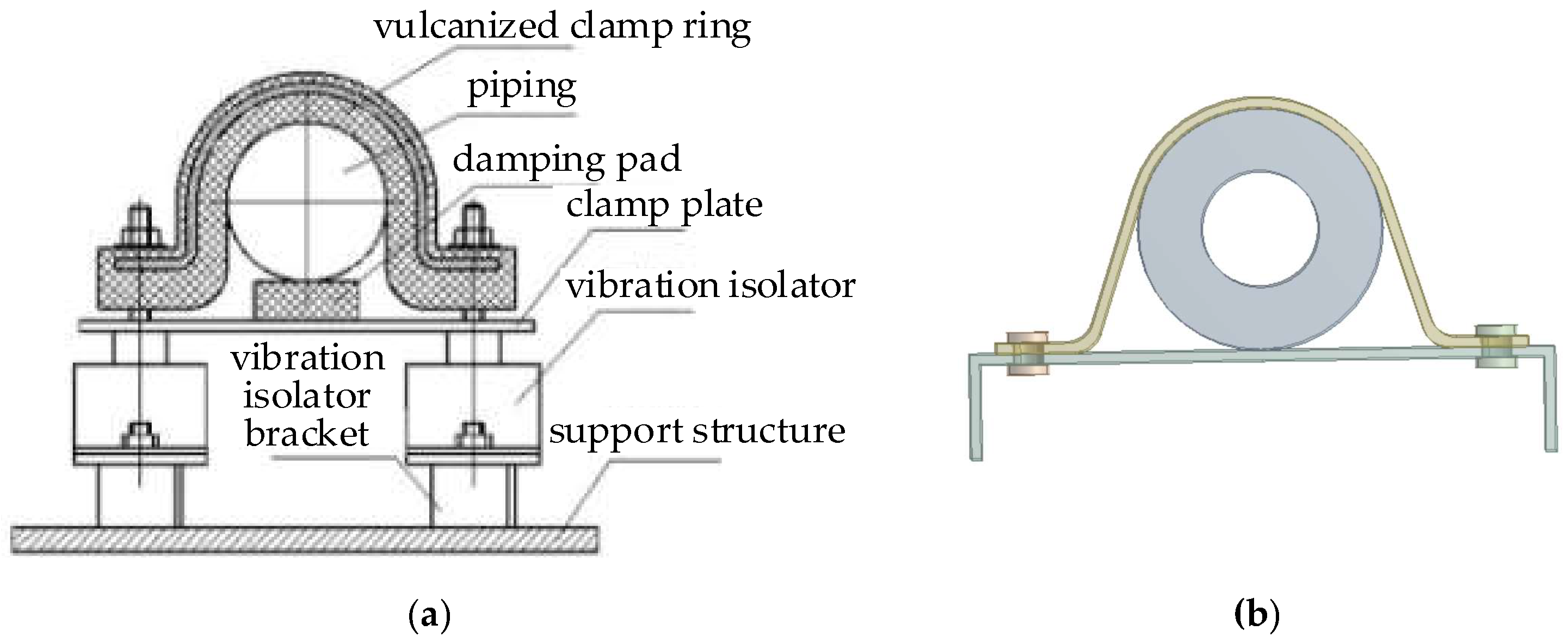
4.1.2. Establishment of a Clamp Dynamics Model for Submarine Hydraulic Pipelines

An accurate dynamic model is the key to analyzing the FSI vibration characteristics of hydraulic pipe systems. When the pipeline vibrates, the interaction between the pipeline, damping pad, clamp plate, and vulcanized clamp ring generates a reaction force, causing deformation to absorb vibration energy and suppress the pipeline vibration, as shown in Figure 8. Therefore, the accurate setting of clamp pre-tightening is crucial for simulating the “pipeline–clamps” system with assembly clearance.

In the actual pre-tightening process of the threaded connectors, the pre-stress should be less than 80% of the material yield point, and the recommended pre-tightening force of the carbon steel bolt is [28,29]:

$$F_0=(0.6~0.7){\sigma }_{\mathrm{s}}{A}_{\mathrm{s}}$$

(4)

where σ_s is the yield limit of the bolt material, (MPa), and A_s is the cross area of bolt stress [30], (mm²).

$$A_{\mathrm{s}}=\frac{\pi }{4}{(\frac{d_2+d_3}{2})}^2$$

(5)

where d₂ is the pitch diameter of the thread, (mm); d₃ is the minor diameter of the thread (d₁) minus 1/6 of the original triangle height of the thread (H), i.e., d₃ = d₁ − H/6, H = 0.866025P, and P is the bolt pitch, (mm).

T = KF₀d

(6)

where T is the torque of the torque wrench, N·m; F₀ is the pre-tightening force of the bolt, N; K is a coefficient, usually taken as 0.18 [31].

In this paper, the material of the bolt is carbon steel, the yield limit of the material is 235 MPa, the stress cross area of the bolt is 15 mm², and the allowable value of the bolt preload is calculated to be 2115~2467.5 N. In the actual pre-tightening of the clamp, the torque measured by the torque wrench is 1.2 N·m. According to Equation (6), the bolt preload is 1111 N, which is less than the maximum allowable preload.

The finite element simulation of bolt pre-tightening is carried out in ABAQUS 6.14. A torque wrench is used to pre-tighten the actual bolt. The pre-tightening torque is 1.2 N·m, and the pre-tightening load of 1111 N is applied to the bolt. Figure 9 shows the stress results of each part of the clamp and bolt.

As can be seen from the stress cloud diagram, there is no reserved gap between the clamp ring and the support in the model. Both of them are steel structures with high stiffness, resulting in the bolt pre-tightening not producing significant compression or tightening effect on the support and the clamp ring (the bolt preload is not transmitted to the external clamp ring and rubber material).

As known from the previous section, the pre-tightening of the clamp mainly reduces the gap between the support and the clamp ring through bolt pre-tightening. The final result is that the assembly gap between the support and the clamp ring is reduced. According to this analysis, based on the existing model, the support is kept in direct contact with the clamp ring, and the interference fit is set between the rubber, the clamp ring, and the support. The interference fit ultimately transfers the force of the clamp ring, compressing the rubber to the pipeline and the support. The process is also consistent with the actual installation situation.

The pre-tightening method is simulated by taking an interference amount of 1 mm, and the final stress and deformation results are shown in Figure 10.

The results show that the maximum stress occurs in the middle of the support and the clamp ring, and the maximum deformation appears at the top of the rubber ring and the two sides in contact with the clamp ring. The clamp ring compresses the rubber ring by eliminating the assembly gap and transmitting the force to the support. The whole process accords with the mechanical behavior of the actual assembly. It is feasible to use the “interference fit” method based on the existing model. Subsequently, this method will be used to construct a clamp model of the submarine pipeline system.

4.2. Modal Simulation Analysis of Pipelines in Different States

In this paper, the modal simulation of pipelines with different sizes and boundary conditions is carried out to verify the correctness of the equivalent mass FSI method and the clamp pre-tightening simulation method. The free modal simulation is mainly aimed at two types of pipelines. One is the empty pipeline without liquid filling, and the other is the liquid-filled pipeline. The simulation parameters are shown in

Table 4. Pipeline parameter settings in modal simulation analysis.

No.	Outer Diameter × Wall Thickness (mm)	Material	State
right-angle elbow 1	38 × 3.5	stainless steel	empty pipe
straight pipe 2	24 × 3	white copper	liquid-filled
straight pipe 3	25 × 3.5	stainless steel	liquid-filled
right-angle elbow 4	22 × 3	white copper	liquid-filled

. The length of both the straight and right-angle elbow is 1 m, and the elbow bends at the midpoint of the pipeline with a bending angle of 90° and a bending radius of 90 mm.

The first three-order modal simulation results of each pipeline are shown in

Table 5. Statistics of the first three natural frequencies of the pipelines.

No.	Order	Frequency (Hz)	No.	Order	Frequency (Hz)
right-angle elbow 1	1	151.08	straight pipe 2	1	98.13
	2	529.70		2	268.91
	3	577.34		3	522.69
straight pipe 3	1	132.57	right-angle elbow 4	1	72.92
	2	363.17		2	244.23
	3	705.45		3	262.57

.

The pipeline adopts a white copper pipeline with a size of 22 mm × 3 mm in the modal simulation under the constraint of clamps, and the pipeline has 2 or 3 U-shaped clamps installed, respectively. The first-order vibration mode of the pipeline system with the clamps is shown in Figure 11 and Figure 12 (in the actual modal test, the clamp has strong constraints and cannot excite higher-order modes, so only the first-order mode is verified).

It can be seen that with the increase in the number of clamps and the enhancement of the constraint, the first-order natural frequency of the system increases, which is consistent with the theoretical results. Subsequent experiments have also proven the feasibility of the bolt preload simulation method. During the simulation calculation, taking the bolt tightening direction as the z direction, the displacement of the vibration mode in this direction is relatively small under low-order modes, and the vibration deformation mainly occurs in the y direction, which is bending vibration.

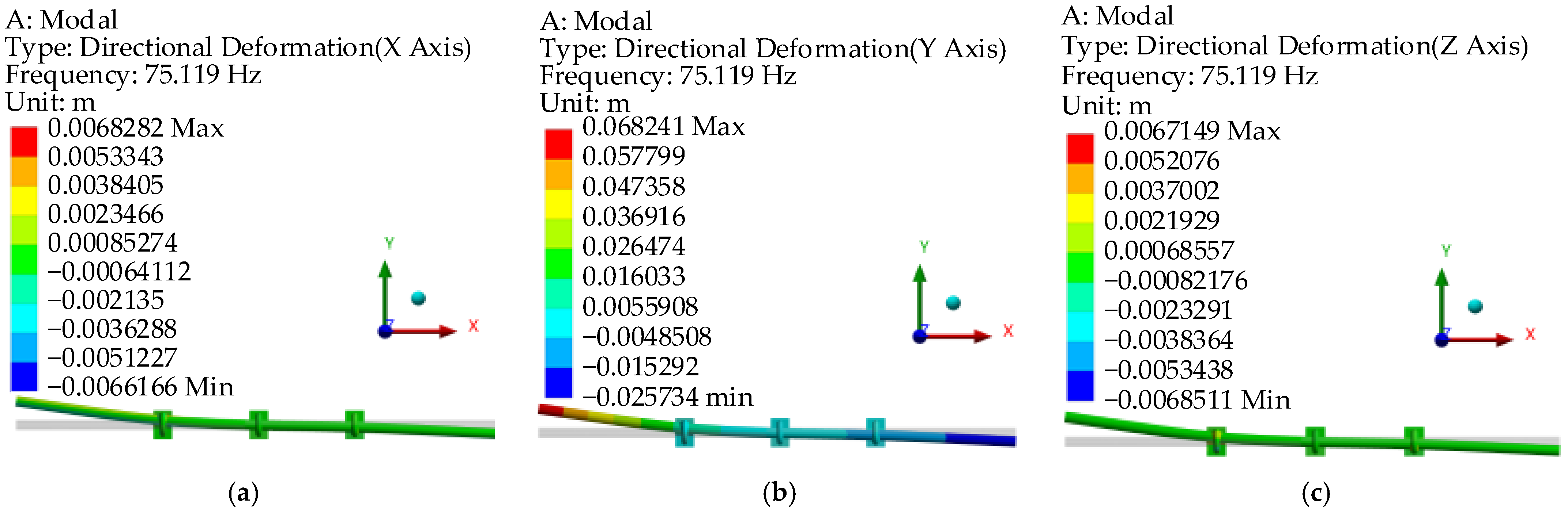
4.3. Analysis of Vibration Characteristics of Hydraulic Pipeline Systems

Due to the long length of the pipeline and the large number of node elements, to improve the calculation efficiency in vibration analysis, water hammer waves (corresponding pressure fluctuations within 0.01 s after closing the valve) during the period with significant fluctuations are used as pipeline vibration excitation.

4.3.1. Analysis of the Vibration Characteristics of the Pipelines at the Pump Source End

The piping system model at the pump source end and the corresponding piping numbers are shown in Figure 13. The pipelines at the pump source have short lengths and high stiffness, so the PL-2, PL-3, and PL-7 pipes, which are greatly affected by water hammer excitation, are selected for vibration characteristics analysis.

For the pipelines in this area, the four ports are connected to other hydraulic accessories. Therefore, the pipeline ports are constrained by fixed supports, and the pipelines and joints use a tie constraint to simulate the threaded connections. The water hammer fluctuation curve of the pipelines at the pump source end is shown in Figure 14, where the water hammer fluctuation in PL-3 and PL-7 is consistent. Under the corresponding water hammer excitation, the stress, deformation, acceleration, and velocity cloud diagrams of the pump source-end pipelines are shown in Figure 15.

Extracting the maximum value of the instantaneous response of the pipelines at the pump source end, the maximum stress is 121.84 MPa, the maximum deformation is 0.085 mm, the maximum vibration acceleration is 179.54 m/s², and the maximum vibration velocity is 0.098 m/s. Among them, the maximum stress appears at the connection between the PL-2 pipeline and the pipe joint, showing a ring stress concentration zone. The occurrence time is consistent with the peak time of water hammer pressure, and the maximum stress is less than the yield strength of stainless steel material. This part is the transition part between the pipe joint and the pipeline, so it bears a large shear stress. The PL-3 pipeline has a larger inner diameter and a variable spatial configuration. The maximum deformation, maximum vibration acceleration, and velocity of the pipelines all appear in the bending part of the pipelines, and the deformation gradient along the pipeline axis is relatively large, indicating that changes in spatial configuration have a significant impact on the deformation.

Through the vibration velocity and acceleration time history curve, it is found that as the water hammer fluctuation gradually decreases, the maximum acceleration and maximum velocity are also gradually decreasing. When the water hammer fluctuation is very small and almost stable, the acceleration and velocity are also close to 0, and the vibration trend is consistent with the water hammer fluctuation trend. The fixed constraint of the pipeline reduces its vibration response and effectively suppresses the pipeline vibration, but increases the stress amplitude and increases the risk of pipeline rupture. In this analysis, the support of the pipeline intersection and tee joint is set as fixed support constraints, which is equivalent to a completely fixed state. Hence, the vibration acceleration and velocity are relatively small. However, it is also found that if it is in a free-floating connection state, the results are exactly the opposite, showing strong vibration acceleration and velocity, which propagate along the pipeline.

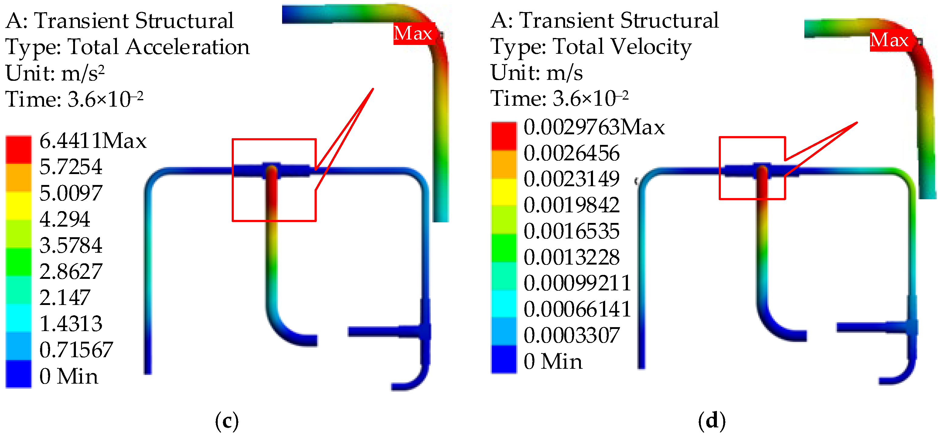
4.3.2. Analysis of the Vibration Characteristics of the Pipelines at the Load End

The pipeline model at the load end model is shown in Figure 16. It includes two sets of identical pressure pipelines and return pipelines and selects pressure pipeline LL-2 for vibration characteristic analysis. When the directional valve is closed, the pressure fluctuation curve of the pressure pipeline after the valve is shown in Figure 17. At the moment of valve closing, the actuator tends to rise under the action of hydraulic force, but there is no hydraulic oil supply, so the pressure in the pipeline decreases in a short time. However, due to gravity, the actuator falls naturally in the opposite direction, compressing the fluid and causing the final pressure to increase and stabilize around 131 bar.

Under the above excitation, the stress, deformation, acceleration, and velocity response cloud diagram of the pressure pipeline at the load end are shown in Figure 18.

Under fluid excitation, the maximum stress of the pipeline is 40.87 MPa, the maximum deformation is 0.109 mm, the maximum vibration acceleration is 74.6 m/s², and the maximum velocity is 0.046 m/s. The maximum vibration response occurs near the location where the spatial configuration of the pipeline changes, and the position is in the middle of the clamps. It can be seen that the vibration response has a maximum value at the bend and gradually decreases on both sides. The vibration response has a large gradient of change along the axial direction of the pipeline.

The above analysis is carried out under the “tie” constraint of the clamps, and it can be seen that the maximum vibration response of the pipeline is concentrated in the bent part. To check the influence of the clamp on the vibration response of the pipeline when the bolt assembly clearance is reduced to achieve the purpose of pre-tightening, the clamp model in this area is re-established. The vibration response of the clamp to the pipeline is mainly reflected in the deformation, and the maximum value of other vibration responses should still appear in the pipeline. This conjecture is also proved in the actual calculation, so only the vibration deformation results are given in Figure 19.

Under the pre-tightening state, the maximum deformation still appears at the bending of the pipeline. However, the current maximum deformation appears in the clamp, and the maximum deformation is 0.33 mm. Under the action of bolt preload, the assembly clearance between the clamp ring and the support is reduced, and the clamp ring compresses the rubber to achieve the constraint effect on the pipeline. After setting the assembly clearance and adding the bolt pre-tightening force, the deformation of the previous maximum deformation position of the pipeline is controlled. The maximum deformation in this area appears on the clamp, and the pre-tightening and constrict effects of the clamp are obvious.

5. Modal Experimental Study on Pipeline Units

This article uses an equivalent quality method for the fluid–structure interaction analysis. Therefore, the pipeline modal test is carried out and compared with the finite element simulation results to verify the correctness of the simulation model.

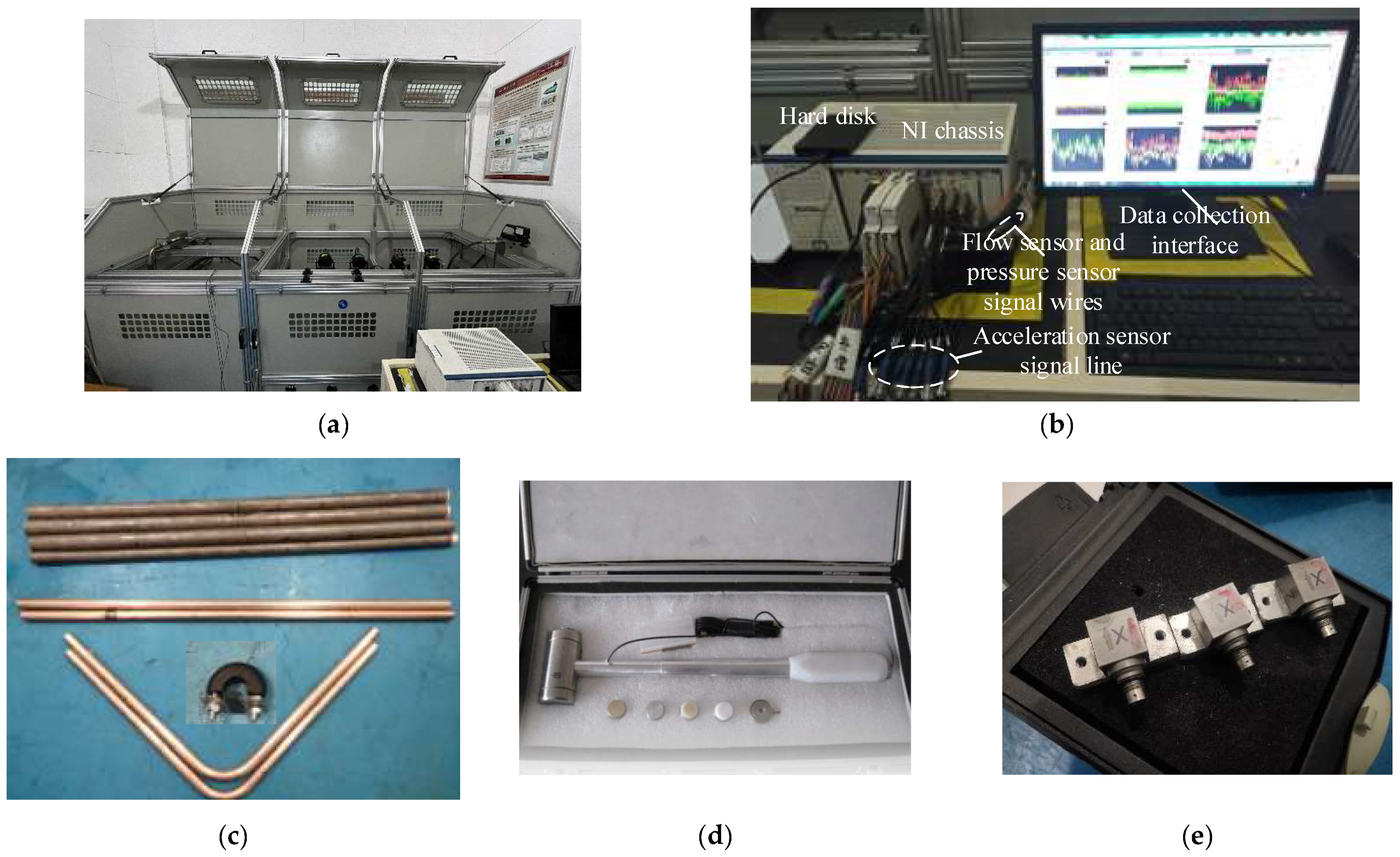
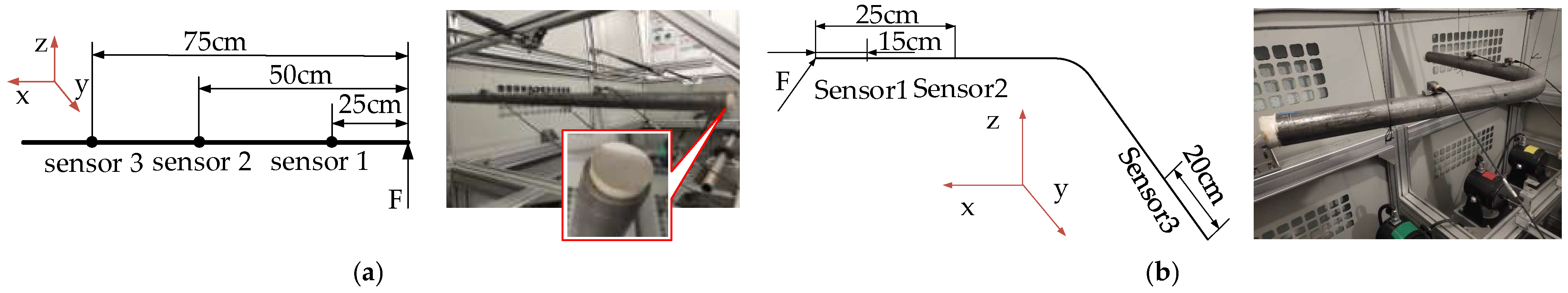
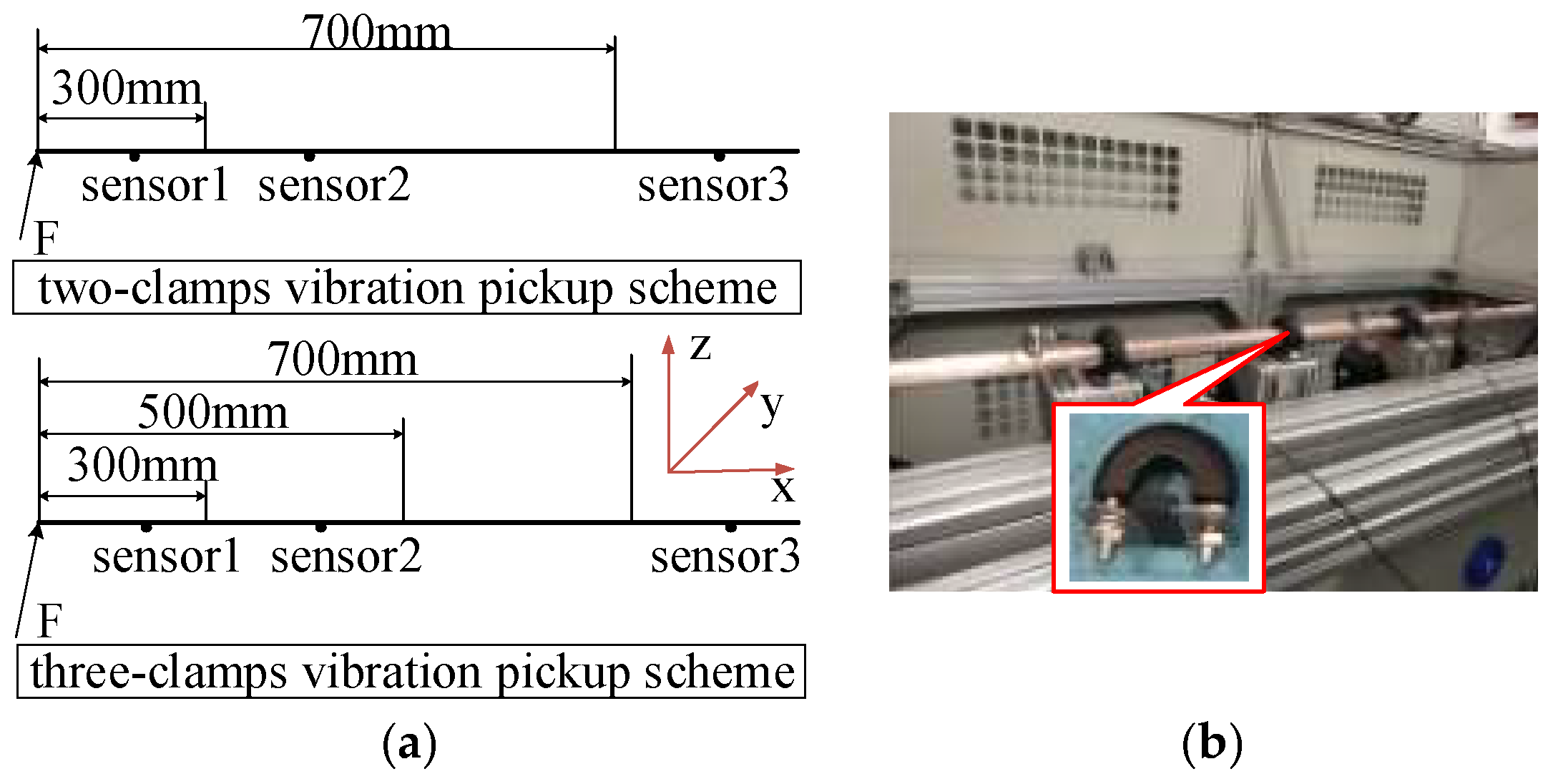
5.1. Construction of Pipeline Modal Test Bench

The modal test object is the pipeline in Table 4. The test bench and measurement system are shown in Figure A1 (Appendix A), and the parameters are shown in

Table A1. The specification of the experimental apparatus and measurement system.

Item	Manufacturer/Type	Performance
Hammer	YDL-2	Charge sensitivity: 4.00 PC/N
		Measuring range: 50 kN
		Linearity: 0.83%
		Natural frequency: 40 kHz
		Resolution ratio: 0.025 N
		Insulation resistance: >1012 Ω
Accelerometer	B&K BK4525-B-001	Measuring range: ±700 m/s2
		Frequency range: 0–20 kHz
		Sensitivity X-axis: 97.04 mV/g Y-axis: 97.21 mV/g Z-axis: 99.00 mV/g
PXIe chassis	National Instruments PXIe-1078	9 AC hybrid slots System slot bandwidth: 250 MB/s System bandwidth: 1 GB/s
PXIe controller	National Instruments PXIe-8820	Dual-core processor (2.2 GHz) System slot bandwidth: 250 MB/s System bandwidth: 1 GB/s
Analog output card	National Instruments PXI-6723	32 analog output channels Conversion rate: 10 kHz Maximum sampling rate: 800 kS/s
Data acquisition card	National Instruments PXI-6221	16 AI channels 2 AO channels Maximum sampling rate: 250 kS/s
Vibration acquisition card	National Instruments PXIe-4497	24 resolution 24 channels Maximum sampling rate: 204.8 kS/s

(Appendix A). The installation of the texted straight pipe is shown in Figure 20.

A single clamp is not enough to fix the pipeline, so in the constraint modal verification test, 2 and 3 clamps are installed separately for analysis. Using an LC-2 hammer to perform fixed-point excitation on one end of the pipeline, the excitation direction is from the outside to the inside along the pipe. Three acceleration sensors are used to collect signals to obtain the vibration acceleration response of the measuring point. The installation of the tested pipeline and the layout of the acceleration sensors are shown in Figure 21.

5.2. Analysis of Modal Verification Test Results for Hydraulic Pipelines

The vibration data of each pipeline are collected, and the time-domain data are Fourier transformed by MATLAB to obtain the frequency response curve of each test piece. The natural frequency value of each pipeline is compared with the simulated value of the finite element method, and the results are shown in

Table 6. Comparison of free-mode natural frequency test values and finite element simulation values.

No.	Parameter	1st-Order	2nd-Order	3rd-Order	No.	Parameter	1st-Order	2nd-Order	3rd-Order
right-angle elbow 1	test value (Hz)	157.71	542.29	601.86	straight pipe 2	test value (Hz)	97.14	264.57	514.19
	simulation value (Hz)	151.08	529.7	577.34		simulation value (Hz)	98.13	268.91	522.69
	error	4.20%	2.32%	4.07%		error	1%	1.6%	1.7%
straight pipe 3	test value (Hz)	129.24	352.24	684.22	right-angle elbow 4	test value (Hz)	70.69	243.83	265.49
	simulation value (Hz)	132.57	363.17	705.45		simulation value (Hz)	72.92	244.23	262.57
	error	2.6%	3.1%	3.1%		error	3.2%	0.16%	1.1%

.

The maximum error is less than 5%. The calculation results are in good agreement with the experimental results, which verifies the correctness of the equivalent density method. This analysis method can be used to conveniently analyze the fluid–structure interaction dynamics, i.e., in some cases, the fluid mass can be equivalent to the pipeline, and the fluid pressure can be applied to the inner wall of the pipeline.

Due to the strong constraints of the clamps, it is difficult to excite multi-order modes using a force hammer. Therefore, only the first-order natural frequency is verified. Compare the first-order natural frequency of pipelines with the finite element simulation value when installing two or three clamps, and the results are shown in

Table 7. Comparison of pipeline-constrained modal tests and numerical simulation results.

Parameter	1st-Order Natural Frequency		Error
	Test Value (Hz)	Simulation Value (Hz)
two clamps	57.86	57.59	0.47%
three clamps	74.14	75.12	1.32%

.

From the final error value, it can be observed that the maximum error is not more than 2%, and the calculation results are in good agreement with the test results, which verifies the correctness of the pipeline constraint in the finite element simulation. At the same time, it can be seen that the natural frequency of the pipeline increases after the number of clamps changes from 2 to 3, which is mainly caused by the increase in constraint stiffness and conforms to the general law.

6. Optimization Analysis of Passive Vibration Control for Pipelines

The passive vibration control optimization analysis is carried out by adjusting the installation position of pipe clamps and taking some pipelines at the load end as an example.

6.1. Parametric Modeling and Co-Simulation

The experimental design is based on the central combination design method. The test results are fitted by the response surface method, and the function is applied to the genetic algorithm for optimizing the position of the clamps. It is necessary to establish a parametric pipeline model to ensure the real-time update of the assembly position of the clamp and improve computational efficiency.

Based on parameterized modeling, Solid Works (SW) and ANSYS are selected for co-simulation. ANSYS CAD Configuration Manager is used to establish an interface between the two softwares. When modeling in SW, the position of clamps is taken as a variable, and a prefix of “DS_” is added before the assembly size name to enable ANSYS to recognize the independent variable. Then, in the optimization process, ticking the target variable is sufficient to achieve real-time updates of the 3D model, greatly improving computational efficiency.

6.2. Optimizing Variables and Objectives

The main target structure of passive vibration control optimization is shown in Figure 22, which is the LL-2 pipeline unit at the load end, equipped with three clamps.

The design variables are the positions of three clamps, and the specific optimization parameter range is shown in

Table 8. Design variable values.

Design Variable	d1	d2	d3
Value range (mm)	4.5~250	4.5~860	4.5~920

.

The optimization goal is the maximum stress of the pipeline, and the ultimate goal is to reasonably optimize the position of the clamp so that the maximum stress value of the pipeline is minimal under a certain fluid excitation.

6.3. Analysis of Optimization Results

A total of 15 groups of design points are generated by the central combination design method. The corresponding clamp position and maximum stress results are shown in

Table 9. Sample points and calculation results.

Design Point	d1 (mm)	d2 (mm)	d3 (mm)	Maximum Stress (×107 Pa)
1	127.25	432.25	462.25	4.6429
2	4.5	432.25	462.25	4.6933
3	250	432.25	462.25	4.6966
4	127.25	4.5	462.25	4.6352
5	127.25	860	462.25	4.7765
6	127.25	432.25	4.5	4.749
7	127.25	432.25	920	4.6245
8	27.45	84.475	90.084	4.7115
9	227.05	84.475	90.084	4.6216
10	27.45	780.03	90.084	4.8336
11	227.05	780.03	90.084	4.7835
12	27.45	84.475	834.42	4.6575
13	227.05	84.475	834.42	4.6179
14	27.45	780.03	834.42	4.7665
15	227.05	780.03	834.42	4.6778

.

Accordingly, Kriging response surface analysis is carried out, i.e., the quadratic regression equation is used to fit the functional relationship between factors and response values. The response surface is obtained, as shown in Figure 23. The response surface reflects the quality of the fitting effect, which will directly determine the quality of the final optimization results. It can be seen from Figure 23 that most design points are located on the response surface, and the fitting results are reliable.

Taking the maximum stress of the vibration response as the optimization objective, the genetic algorithm is used to optimize the position of the clamps, and three groups of candidate points are obtained. The error in verification results is shown in

Table 10. Optimization results and verification.

Candidate Point	d1 (mm)	d2 (mm)	d3 (mm)	Maximum Stress (×107 Pa)	Verification Stress (×107 Pa)	Error/%
1	249.66	415	871.62	4.048	4.5059	10.16
2	249.85	409.87	864.98	4.182	4.5069	7.21
3	248.8	395.18	892.5	3.921	4.2078	6.82

.

The optimized candidate points are verified. The maximum error between the obtained results and the optimized prediction results is about 10%, and the error is small. Compared with the results of each design point and the maximum stress of the initial vibration of the pipeline, the maximum stress is significantly reduced; that is, the passive vibration control optimization based on the genetic algorithm plays a certain role.

After optimization, the value of d₁ is extreme. The corresponding clamp moves away from the right-angle bend of the pipeline, and within its allowable movement range, it is extremely close to the bending of the pipeline. The corresponding clamp of d₂ is finally stable in the middle of the movable range. Considering the previous vibration analysis results, the bending part of the pipeline is often the stress concentration site, and the clamp is between the two bending parts. Therefore, the clamp may be arranged in the middle to better disperse the influence of stress concentration. The final optimized position of the clamp corresponding to d₃ is at the fixed support of the pipeline, which tends to produce stress concentration, especially in the inner wall of the nearby pipeline, where the stress amplitude or stress propagation is larger and wider. From the data analysis, the stress at the fixed support is greater than the optimized stress value, so the clamp placed at the fixed support can play a role in reducing the stress concentration. Among the above three candidate points, the maximum stress of the pipeline is 41.82 MPa, which is less than the yield strength of the white copper material and meets the requirements of use.

7. Conclusions

In this paper, through theoretical analysis, simulation research, and experimental verification of the water hammer and vibration characteristics of the submarine local hydraulic system, the following conclusions can be drawn:

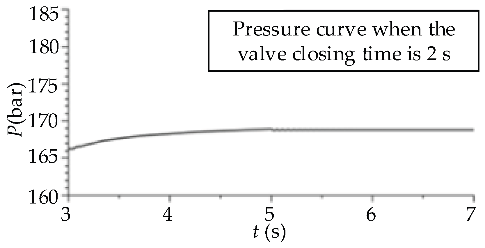
• The shorter the commutation time of the directional valve, the more severe the water hammer fluctuation is. When the commutation time is large enough, the water hammer wave will not produce intense fluctuations but will increase steadily to a higher pressure.
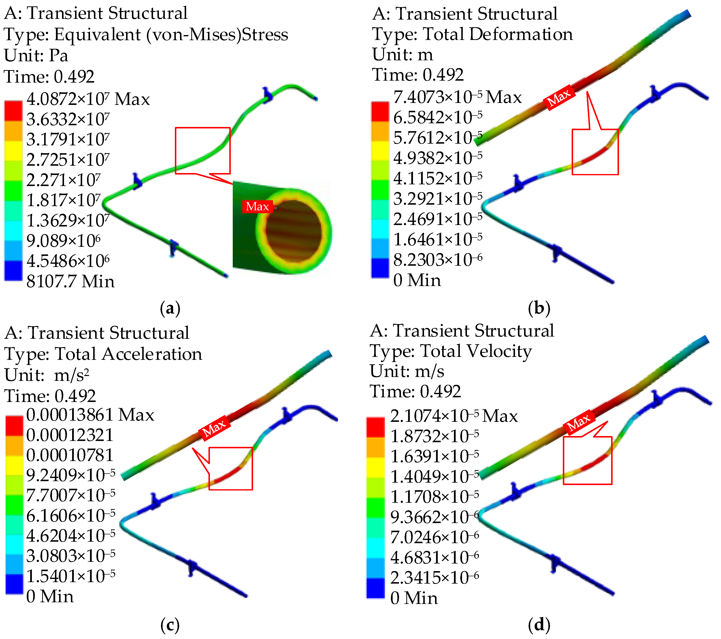
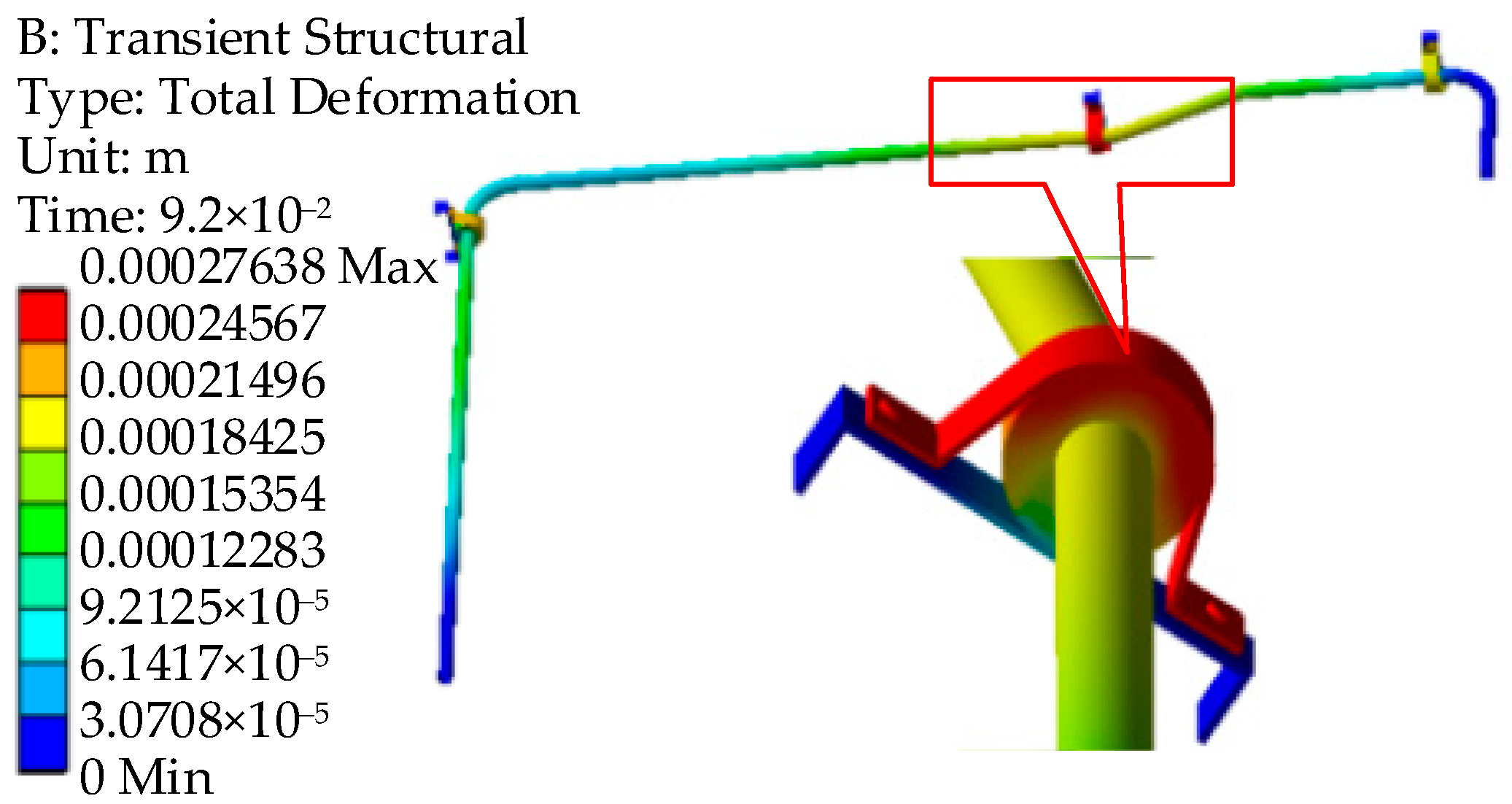
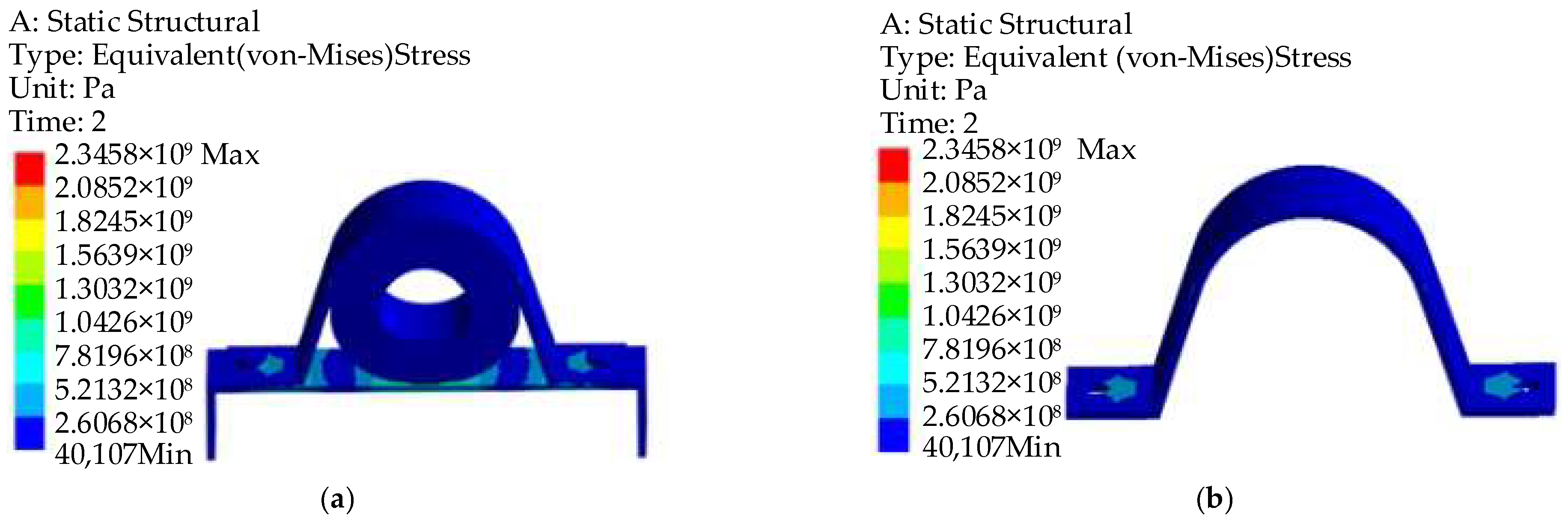
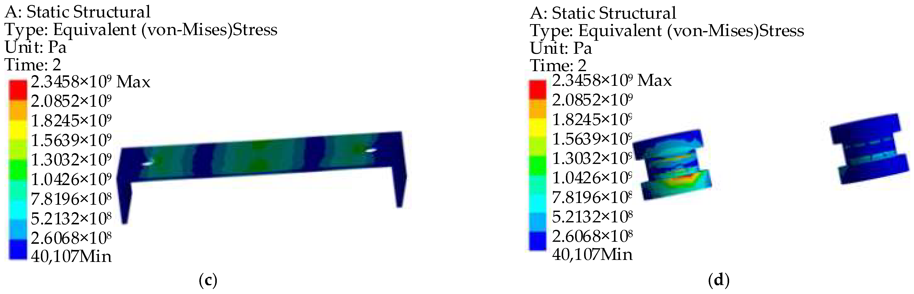
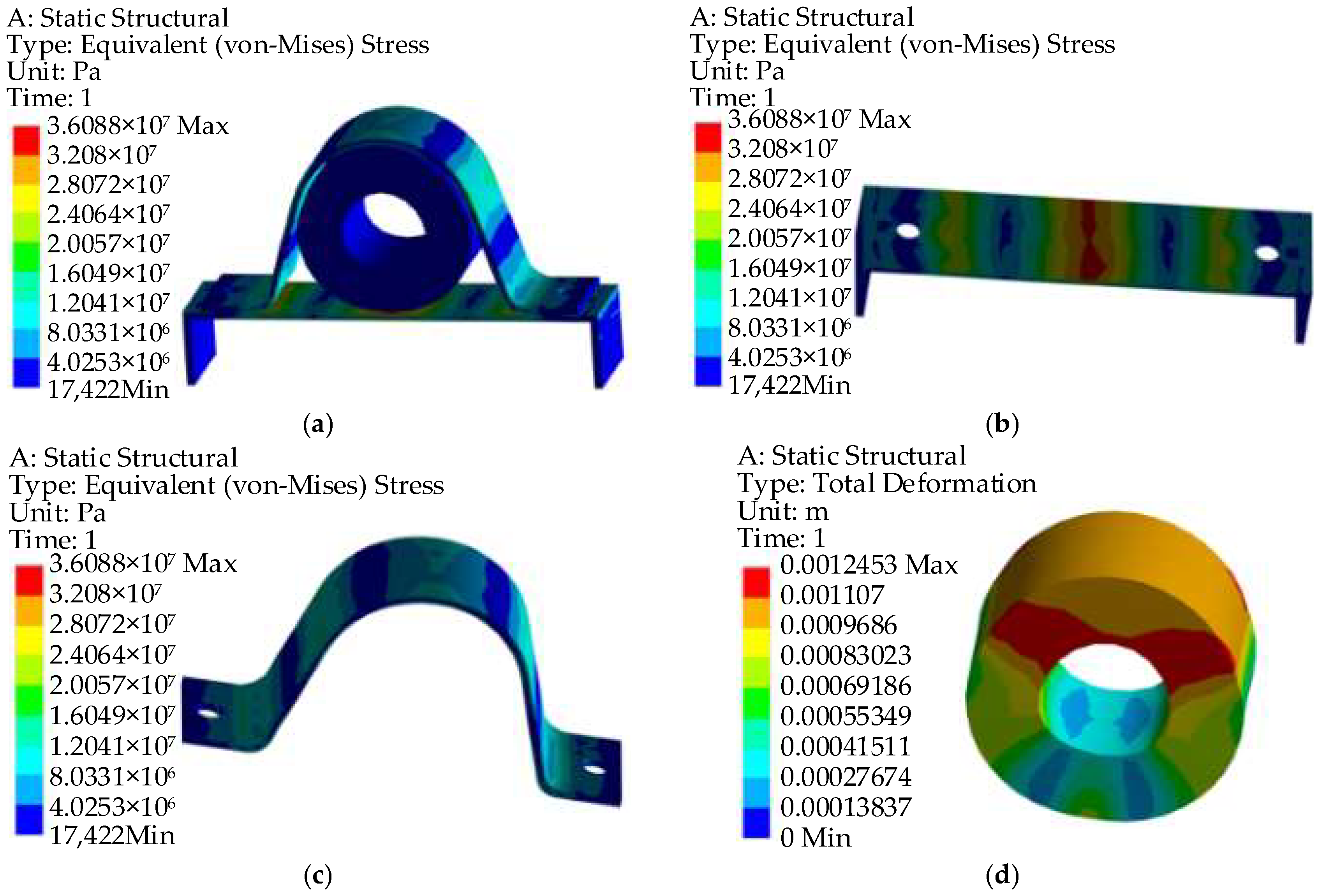
• The maximum vibration response of the pipeline under water hammer excitation mostly occurs at the position where the pipeline configuration changes, and the vibration stress has the same change trend as the fluid excitation. Under the water hammer excitation, the pipelines can meet the strength requirements.
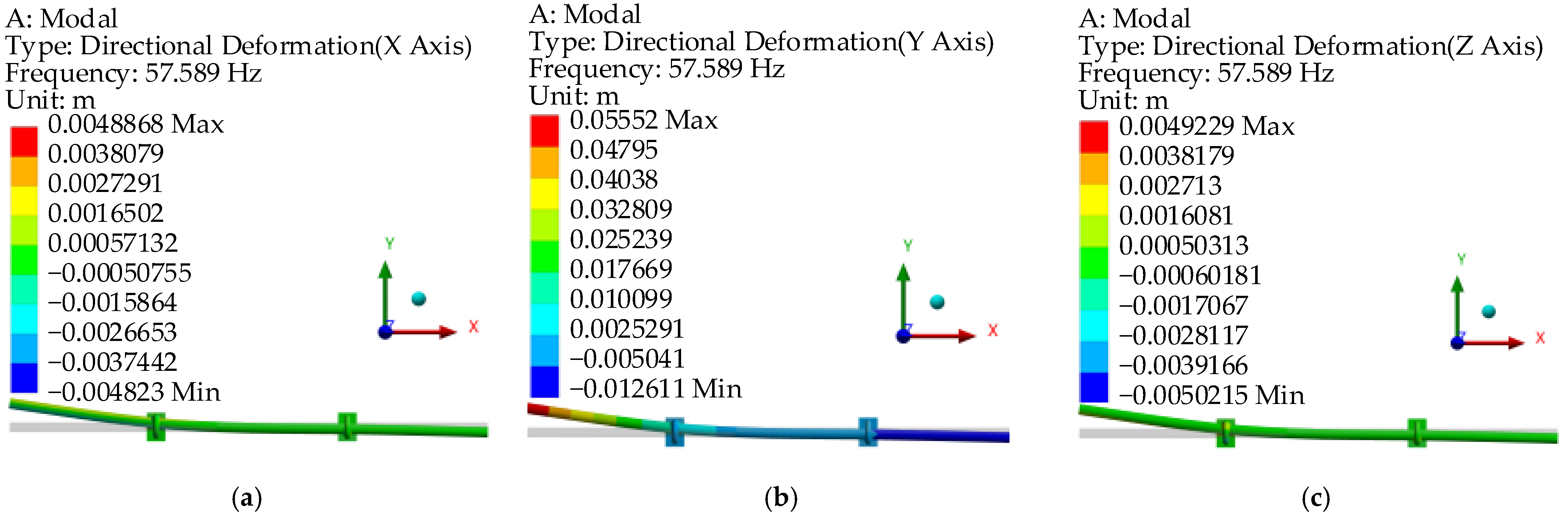
• The modal finite element analysis and experimental verification of the pipeline are carried out. The results show that the error between the finite element calculation and the experimental results is within 5%. The structural stiffness (simulating bolt pre-tightening through interference fit) and mass (fluid density equivalent) related settings that have a significant influence on the modal are preliminary verified in this paper.
• The genetic algorithm is used to optimize the clamp layout. The difference between the predicted optimization results and the actual analysis results is within 5%, indicating that the optimization analysis method is feasible. Through optimization analysis, it is determined that the arrangement of the clamps should be close to the fixed support of the pipeline to avoid small areas of stress concentration.
• In this study, vibration analysis only considers the influence of the water hammer. In future work, the multi-source vibration modeling and analysis of the submarine hydraulic pipeline system should be constructed. Additionally, the multi-source vibration superposition mechanism and transmission law of the actuator, hydraulic valve, pipeline support, and hull should be studied in depth.

References

1. Quan, L.X.; Kong, X.D.; Yu, B.; Bai, H.H. Research Status and Trends on Fluid-Structure Interaction Vibration Mechanism and Control of Hydraulic Pipeline. J. Mech. Eng. 2015, 51, 175–183. [Google Scholar] [CrossRef]
2. Cai, Y.G. Pipeline Dynamics of Fluid Transmission; Zhejiang University Press: Hangzhou, China, 1990. [Google Scholar]
3. Pal, S.; Hanmaiahgari, P.R.; Karney, B.W. An Overview of the Numerical Approaches to Water Hammer Modelling: The Ongoing Quest for Practical and Accurate Numerical Approaches. Water 2021, 13, 1597. [Google Scholar] [CrossRef]
4. Zhang, D.S. Effect of Unsteady Friction and Valve Closing Law on Water Hammer. Master’s Thesis, Xi’an University of Technology, Xi’an, China, June 2021. [Google Scholar]
5. Jiang, D.; Lu, Q.; Liu, Y.; Zhao, D. Study on Pressure Transients in Low Pressure Water-Hydraulic Pipelines. IEEE Access 2019, 7, 80561–80569. [Google Scholar] [CrossRef]
6. Liu, Y. Research on Water Hammer Suppression Method Based on Valve Closing Rule in Hydraulic Pipeline. Master’s Thesis, University of Electronic Science and Technology of China, Chengdu, China, June 2021. [Google Scholar]
7. Chen, Y.; Zhao, C.; Guo, Q.; Zhou, J.; Feng, Y.; Xu, K. Fluid-Structure Interaction in a Pipeline Embedded in Concrete During Water Hammer. Front. Energy Res. 2022, 10, 956209. [Google Scholar] [CrossRef]
8. Afshar, M.H.; Rohani, M. Water hammer simulation by implicit method of characteristic. Int. J. Press. Vessel. Pip. 2008, 85, 851–859. [Google Scholar] [CrossRef]
9. Mikota, G. Low Frequency Correction of a Multi-Degrees-of-Freedom Model for Hydraulic Pipeline Systems. IFAC-PapersOnLine 2015, 48, 435–440. [Google Scholar] [CrossRef]
10. Mikota, G.; Manhartsgruber, B.; Kogler, H.; Hammerle, F. Modal Testing of Hydraulic Pipeline Systems. J. Sound Vib. 2017, 409, 256–273. [Google Scholar] [CrossRef]
11. Sadat Hosseini, R.; Ahmadi, A.; Zanganeh, R. Fluid-Structure Interaction during Water Hammer in a Pipeline with Different Performance Mechanisms of Viscoelastic Supports. J. Sound Vib. 2020, 487, 115527. [Google Scholar] [CrossRef]
12. Ulanov, A.M.; Bezborodov, S.A. Calculation Method of Pipeline Vibration with Damping Supports Made of the MR Material. Procedia Eng. 2016, 150, 101–106. [Google Scholar] [CrossRef]
13. Bezborodov, S.A.; Ulanov, A.M. Calculation of Vibration of Pipeline Bundle with Damping Support Made of MR Material. Procedia Eng. 2017, 176, 169–174. [Google Scholar] [CrossRef]
14. Chai, Q.D.; Zeng, J.; Ma, H.; Li, K.; Han, Q.K. Dynamic Modeling Approach for Nonlinear Vibration Analysis of the L–Type Pipeline System with Clamps. Chin. J. Aeronaut. 2020, 33, 3253–3265. [Google Scholar] [CrossRef]
15. Chai, Q.D.; Fu, Q.; Ma, H.; Han, Q.K.; Zhang, D.Z. Modeling and Dynamic Characteristics Analysis for a Pipeline System with Single Double–Clamp. J. Vib. Shock. 2020, 39, 114–120. [Google Scholar]
16. Chai, Q.D.; Piao, Y.H.; Ma, H.; Wu, W.X.; Sun, W. Calculation of Natural Characteristics and Experimental Methods of the Clamp-Pipe System. J. Aerosp. Power 2019, 34, 1029–1035. [Google Scholar]
17. Gao, P.; Yu, T.; Zhang, Y.; Wang, J.; Zhai, J. Vibration Analysis and Control Technologies of Hydraulic Pipeline System in Aircraft: A Review. Chin. J. Aeronaut. 2021, 34, 83–114. [Google Scholar] [CrossRef]
18. Wang, Y.; Huang, Y.X.; Li, S.M. Vibration Analysis and Optimization of Aircraft Engine Driven Pump Outlet Pipeline. Chin. Hydraul. Pneum. 2020, 9, 115–121. [Google Scholar]
19. Liu, X.F.; Zhang, Y.L.; Zhang, D.C.; Yu, T.; Gao, P.X. Analysis and Test Verification of Stiffness and Damping Characteristics of Aviation Clamp with Cushion. J. Aerosp. Power 2022, 37, 274–282. [Google Scholar]
20. Li, X.; Li, W.H.; Shi, J.; Li, Q.; Wang, S.P. Pipelines Vibration Analysis and Control Based on Clamps’ Locations Optimization of Multi-Pump System. Chin. J. Aeronaut. 2022, 35, 352–366. [Google Scholar] [CrossRef]
21. Quan, L.X.; Zhang, Q.W.; Li, Z.C.; Sheng, S.W. Sensitivity Analysis and Optimization for Support Parameter of Aviation Hydraulic Pipeline. Chin. Hydraul. Pneum. 2017, 8, 95–99. [Google Scholar]
22. Frahm, H. Device for Damping Vibrations of Bodies. Google Patents US989958A, 18 April 1911. [Google Scholar]
23. Jiang, J.; Lou, J.; Deng, F. Control Measures about Vibration and Noise of Pipeline Onboard Marine Vessels. Vibroeng. Procedia 2015, 5, 377–382. [Google Scholar]
24. Song, G.B.; Zhang, P.; Li, L.Y.; Singla, M.; Patil, D.; Li, H.N.; Mo, Y.L. Vibration control of a pipeline structure using pounding tuned mass damper. J. Eng. Mech. 2016, 142, 4016031. [Google Scholar] [CrossRef]
25. Zhang, X.; Bian, S.; Wang, H.; Jia, X.; Wang, C. Effects of Valve Opening on Direct Water Hammer Pressure Characteristics in PMMA Pipelines. J. Braz. Soc. Mech. Sci. Eng. 2023, 45, 408. [Google Scholar] [CrossRef]
26. Arefi, M.H.; Ghaeini-Hessaroeyeh, M.; Memarzadeh, R. Numerical Modeling of Water Hammer in Long Water Transmission Pipeline. Appl. Water Sci. 2021, 11, 140. [Google Scholar] [CrossRef]
27. Ye, J.; Zeng, W.; Zhao, Z.; Yang, J.; Yang, J. Optimization of Pump Turbine Closing Operation to Minimize Water Hammer and Pulsating Pressures During Load Rejection. Energies 2020, 13, 1000. [Google Scholar] [CrossRef]
28. Liu, Z.; Wang, D.; Cheng, P.; Zang, Y. Research on Non-Contact Bolt Preload Monitoring Based on DIC. J. Phys. Conf. Ser. 2023, 1, 2528. [Google Scholar] [CrossRef]
29. Pu, L.; Ji, M. Mechanical Design, 8th ed.; Higher Education Press: Beijing, China, 2006. [Google Scholar]
30. Wang, B. Fluid-Structure Interaction Dynamic Analysis of the Typical Aircraft Hydraulic Pipeline. Master’s Thesis, Xi’an University of Technology, Xi’an, China, June 2013. [Google Scholar]
31. Thomas, P.S. Analysis of Induced Vibrations in Fully-developed Turbulent Pipe Flow Using a Coupled LES and FEA Approach; Brigham Young University: Provo, UT, USA, 2009. [Google Scholar]
Figure 1. Schematic diagram of the local hydraulic system.
Jmse 11 01885 g001
Figure 2. Topological structure division of the hydraulic system.
Jmse 11 01885 g002
Figure 3. Local hydraulic system flow and pressure calculation model.
Jmse 11 01885 g003
Figure 4. Water hammer fluctuation curve at node 1 under different valve closing times.
Jmse 11 01885 g004
Figure 5. Pressure curve when the valve closing time is 2 s.
Jmse 11 01885 g005
Figure 6. Water hammer transmission and attenuation result at different valve closing times. Water hammer curve of three nodes when the valve closing times are (a) 0.01 s; (b) 0.03 s; (c) 0.05 s; (d) 0.1 s.
Jmse 11 01885 g006
Figure 7. Correlation curve between system friction and valve closing process.
Jmse 11 01885 g007
Figure 8. Clamp structure diagram. (a) Two-dimensional drawing; (b) finite element model.
Jmse 11 01885 g008
Figure 9. Stress cloud diagram under bolt pre-tightening. (a) The overall stress cloud diagram of the clamp; (b) clamping ring stress cloud diagram; (c) support stress cloud diagram; (d) bolt stress cloud diagram.
Jmse 11 01885 g009aJmse 11 01885 g009b
Figure 10. Stress and deformation cloud diagram under interference preloading. (a) The overall stress cloud diagram of the clamp; (b) support stress cloud diagram; (c) clamping ring stress cloud diagram; (d) rubber ring deformation cloud diagram.
Jmse 11 01885 g010
Figure 11. First-order vibration mode of the pipeline with two clamps. (a) X-axis; (b) Y-axis; (c) Z-axis.
Jmse 11 01885 g011
Figure 12. First-order vibration mode of the pipeline with three clamps. (a) X-axis; (b) Y-axis; (c) Z-axis.
Jmse 11 01885 g012
Figure 13. The piping system model at the pump source end.
Jmse 11 01885 g013
Figure 14. Water hammer excitation curve in the pump source-end pipelines.
Jmse 11 01885 g014
Figure 15. Vibration response cloud diagram of pump source-end pipelines. (a)Stress cloud diagram; (b) deformation cloud diagram; (c) acceleration cloud diagram; (d) velocity cloud diagram.
Jmse 11 01885 g015aJmse 11 01885 g015b
Figure 16. The piping system model at the load end.
Jmse 11 01885 g016
Figure 17. The pressure fluctuation curve of pressure pipelines at the load end.
Jmse 11 01885 g017
Figure 18. Vibration response cloud diagram of pipelines at the load end. (a) Stress cloud diagram; (b) deformation cloud diagram; (c) acceleration cloud diagram; (d) velocity cloud diagram.
Jmse 11 01885 g018
Figure 19. The deformation results under pre-tightening assembly.
Jmse 11 01885 g019
Figure 20. Installation of the liquid-filled pipeline. (a) Installation diagram of the straight pipeline; (b) Installation diagram of the elbow.
Jmse 11 01885 g020
Figure 21. Installation of the tested pipeline in the constrained modal test. (a) Vibration pickup scheme and installation diagram; (b) actual installation diagram.
Jmse 11 01885 g021
Figure 22. LL-2 Pipeline Unit.
Jmse 11 01885 g022
Figure 23. Response surface.
Jmse 11 01885 g023