Numerical Analysis on Influences of Emergent Vegetation Patch on Runup Processes of Focused Wave Groups

Abstract

During severe weather, the runup of the devasting surges and waves can cause extensive damages to the coastal facilities and results in significant loss of life. Therefore, it becomes necessary to find reliable measures to reduce the wave runup in coastal regions. As a natural barrier to the shorelines, coastal vegetation has great potential to attenuate wave runup and to prevent the coastal communities from extreme floodings and huge land loss. This study numerically discusses the influences of the emergent vegetation patch on the runup processes of extreme wave groups by applying a nonhydrostatic flow solver. Influences of the major factors, i.e., water depth, peak wave period, significant wave height, and density and length of the vegetation patch, are analyzed in detail. Research findings indicate that the presence of the emergent vegetation patch can substantially dissipate most of the incident wave energy and effectively reduce the maximum wave runup heights of extreme wave groups at the sloped beach. It is hoped that the research results of this study will be helpful to the design of coastal soft protection measures.

1. Introduction

During severe weather events, wave runup of the devasting surges and waves can cause massive damages to the coastal facilities and results in significant loss of life [1,2,3]. Therefore, it is necessary to find reliable measures to reduce the wave runup in the coastal regions. Traditionally, hard protection measures, i.e., seawall and breakwaters, were widely constructed along coastlines to mitigate the adverse impacts of wave runup [4]. However, they are not only expensive to construct and maintain, but also tend to have negative impacts on the environment [5], i.e., deterioration of water quality and sediment deposition. As a natural barrier to the shorelines, coastal vegetation has great potential to attenuate the wave runup and to prevent coastal communities from the destructive floodings and serious land loss [6,7,8,9], which has been confirmed by many post-disaster surveys [10,11,12,13]. Meanwhile, aquatic vegetation also has positive impacts on the coastal ecological system, i.e., providing the habitat for a wide variety of organisms [14] and reducing coastal erosion [15,16]. However, due to the complexity of wave–vegetation interactions, influences of coastal vegetation on the wave runup processes of different types of incident waves have not been adequately understood.

In the past, extensive field surveys [10,11,12,13,17], theoretical analysis [18,19], laboratory experiments [20,21], and numerical simulations [22,23] were conducted to assess the wave attenuation properties of the various types of coastal vegetation, i.e., mangroves [24], saltmarshes [25], and seagrass [26]. The post-disaster investigation conducted by Kandasamy and Rajendran [10] at the southeastern coast of India after the 2004 Indian Ocean Tsunami revealed the significant importance of mangroves in reducing the extreme surges and waves. Further investigations found that coastal regions with dense mangroves suffered significantly less damage than the coastal regions without the vegetation protection [27]. By applying linear wave theory and Morrison equations [28], Dalrymple et al. [18] proposed a theoretical model to predict the wave dissipation of a vegetation patch composed of vertical vegetation cylinders. This classical theoretical model was further improved to account for the influences of wave breaking processes [29] and wave–current interactions [30] in recent years. In addition, scholars had also put forward some other theoretical models, i.e., mild-slope model [31] and spectral-action balance model [32]. Meanwhile, many laboratory experiments were carried out to study the wave attenuation of emergent vegetation under solitary waves [22,23], regular waves [33,34], and irregular waves [35]. Complicated interactions between the solitary wave and emergent vegetation patch at the seabed were experimentally analyzed by Huang et al. [22]. Based on their collected experiment data, an empirical formula was proposed to predict the drag coefficient of vegetation stem. Influences of current on the wave attenuation of real-vegetation patches were investigated by Rupprecht et al. [36]. The wave attenuation properties of the complex combination of canopy, stem, and root were systematically analyzed by He et al. [37]. Moreover, the performance of submerged vegetation patch and suspended vegetation patch in attenuating the ocean surface waves have been also extensively studied [38,39,40,41] by laboratory experiments.

In the past two decades, various types of the numerical models were applied to study the complexity of wave–vegetation interactions [24,42,43,44]. For instance, by applying an improved Boussunesq wave model, the wave attenuation properties of flexible and rigid vegetation patches were systematically analyzed by Augustin et al. [45] and Huang et al. [22]. In addition, the hydrodynamic processes of ocean surface waves in the vegetation patches were also numerically simulated by applying the shallow water equations [46,47,48]. Nevertheless, the complex flow field within the wave–vegetation interactions often contains strong vertical accelerations, which beyond the computational capability of the Boussinesq wave model and the nonlinear shallow water models [49]. In recent years, the nonhydrostatic wave models were widely applied to assess the wave attenuation properties of coastal vegetation under the solitary wave, regular waves, irregular waves, and even the real-word tsunami waves [8,9]. For instance, by applying the nonhydrostatic wave model, Suzuki et al. [50] analyzed the influences of drag and inertia forces and the porosity of vegetation on the wave attenuation. Moreover, two-phase flow models were also applied to study the turbulent dissipations in the vegetation region [51], wave breaking at the vegetated beach [52], and the wave attenuation of the submerged and emergent vegetation patches [53]. Although the previous research greatly advanced our understandings on the wave attenuation properties of coastal vegetation, the research on the influences of coastal vegetation on wave runup is inadequate. Irtem et al. [54] investigated the attenuation effects of artificial trees on the wave runup processes of a tsunami wave at a sandy beach. Effects of the open gap of the coastal vegetation on the runup of tsunami waves were analyzed by Thuy et al. [55]. Later, influences of the vegetation density on the wave runup were discussed by Iimura et al. [23] and Yao et al. [56]. By applying the shallow water model, Tang et al. [57] and Zhang et al. [58] studied the wave runup and land flooding processes at the vegetated sloped beach. The runup of real-world tsunami waves on the vegetated beach was analyzed by Sun et al. [9].

A focused wave is also an irregular wave, which contains many wave components with different amplitudes, periods, and phases. When these wave components focus together at specific locations and times, the maximum water elevations of all wave components can add up to a large wave height. In the real-harsh coastal environment, although the focused waves often occur unexpectedly, their large wave heights can cause massive damages to the coast [59] and impose huge impacting loads at coastal infrastructures, i.e., cylinders [60], seawall [61], and bridges [62]. Recently, complicated interactions between the focused wave groups and emergent rigid vegetation patch on the flat bed were investigated by Qu et al. [63]. However, influences of coastal vegetation on the wave runup processes of the focused wave group have not been well understood. In this study, effects of the emergent vegetation patch on the runup processes of the focused waves were systematically investigated using a nonhydrostatic flow solver (NHWAVE) [64]. Influences of the major factors, i.e., water depth, peak wave period, significant wave height, and density and length of the vegetation patch, are discussed in detail. The rest of this paper is organized as follows. Section 2 gives the descriptions on the numerical wave model. Section 3 introduces the generating method of the focusing wave. Definitions of some parameters related to the wave attenuation are described in Section 4. Model validations are performed in Section 5. Section 6 discusses the influences of the emergent vegetation on the runup processes of the focused wave groups. Conclusions are presented in Section 7.

2. Descriptions on Numerical Wave Model

The runup processes of focused wave groups and their complex interactions with the emergent rigid vegetation patch can be fully described by the incompressible flow, whose governing equations can be formulated as

$$\frac{\partial D}{\partial t}+\frac{\partial Du}{\partial x}+\frac{\partial Dv}{\partial y}+\frac{\partial \omega }{\partial \sigma }=0$$

(1)

$$\frac{\partial U}{\partial t}+\frac{\partial F}{\partial x}+\frac{\partial G}{\partial y}+\frac{\partial H}{\partial \sigma }=S_h+S_p+S_{\tau }+S_v$$

(2)

where $U=\left(Du,Dv,Dw\right)$, and the well-balanced fluxes are formulated as

$$F=\left(\begin{array}{c}Duu+\frac{1}{2}g{\eta }^2+gh\eta \\ Duv\\ Duw\end{array}\right)G=\left(\begin{array}{c}Duv\\ Dvv+\frac{1}{2}g{\eta }^2+gh\eta \\ Dvw\end{array}\right)H=\left(\begin{array}{c}u\omega \\ v\omega \\ w\omega \end{array}\right)$$

and the flux terms on the right side of Equation (2) are

$$S_h=\left(\begin{array}{c}gD\frac{\partial h}{\partial x}\\ gD\frac{\partial h}{\partial y}\\ 0\end{array}\right)S_p=\left(\begin{array}{c}-\frac{D}{\rho }\left(\frac{\partial p}{\partial x}+\frac{\partial p}{\partial \sigma }\frac{\partial \sigma }{\partial x}\right)\\ -\frac{D}{\rho }\left(\frac{\partial p}{\partial y}+\frac{\partial p}{\partial \sigma }\frac{\partial \sigma }{\partial y}\right)\\ -\frac{1}{\rho }\frac{\partial p}{\partial \sigma }\end{array}\right)S_{\tau }=\left(\begin{array}{c}D{S}_{{\tau }_x}\\ D{S}_{{\tau }_y}\\ D{S}_{{\tau }_z}\end{array}\right) S_v=\left(\begin{array}{c}D\left(f_{dx}+f_{vmz}\right)\\ D\left(f_{dy}+f_{vmz}\right)\\ D\left(f_{dz}+f_{vmz}\right)\end{array}\right)$$

In the above equations, $t$ is time; $x, y, \mathrm{and} z$ represent the Cartesian coordinates; $u, v, \mathrm{and} w$ are the corresponding velocities in the $x$, $y$, and $z$ directions, respectively; $\omega$ represents the velocity in the $\sigma$ coordinate, and $\sigma =\left(z+h\right)/D$. The total water depth ($D$) is calculated as $D=h+\eta$, and $\eta$ is the water elevation; $h$ is the water depth; $g$ is the acceleration of gravity; $\left|u\right|$ represents the magnitude of the velocity, and $\left|u\right|=\sqrt{u^2+v^2+w^2}$; $p$ is the pressure; $\rho$ is the density. In addition, $D{S}_{{\tau }_x}$, $D{S}_{{\tau }_y},$ and $D{S}_{{\tau }_z}$ are the diffusion source terms.

At present, there exit two main approaches to simulate the vegetation piles. For the first approach, geometries of the vegetation piles can be resolved by the high-resolution computational meshes. The other approach is to simulate the drag forces of vegetation piles, and not to resolve their exact geometries. Since the first approach is a highly computational load, the second approach is applied in this study. The drag forces of vegetation piles are modeled, and are added to the momentum equations. The combined contribution of form drag force ($f_{Fi}$) and viscous force ($f_{Vi}$) of the emergent vegetation patch can be formulated as

$$f_{di}=f_{Vi}+f_{Fi}=\frac{1}{2}{C}_D\lambda u_i\left|u\right|$$

(3)

where $C_D$ is the drag coefficient; $N_v$ represents the number of stems in a unit area; $b_v$ represents the stem diameter; $\lambda =b_v{N}_v$ is defined as the vegetation density. Within the complicated interactions between the focused waves and vegetation patch, the contribution of inertial forces cannot be ignored in the oscillatory flow, which can be formulated as

$$f_{vmi}=C_M\frac{\pi d_v^2}{4}{N}_v\frac{\partial u_i}{\partial t}$$

(4)

The eddy viscosity was calculated by the nonlinear $k$-$\epsilon$ turbulence model [65], whose governing equations can be described as

$$\frac{\partial Dk}{\partial t}+\nabla ·\left(Duk\right)=\nabla ·\left[D\left(\nu +\frac{v_t}{{\sigma }_k}\right)\nabla k\right]+D\left(P_s+C_{fk}{P}_V-\epsilon \right)$$

(5)

$$\frac{\partial D\epsilon }{\partial t}+\nabla ·\left(Du\epsilon \right)=\nabla ·\left[D\left(\nu +\frac{v_t}{{\sigma }_{\epsilon }}\right)\nabla \epsilon \right]+\frac{\epsilon }{k}D\left(C_{1\epsilon }\left(P_s+C_{f\epsilon }{P}_V\right)-C_{2\epsilon }\epsilon \right)$$

(6)

The eddy viscosity $v_t$ is determined by $v_t=C_{\mu }\frac{k^2}{\epsilon }$. ${\sigma }_k$, ${\sigma }_{\epsilon }$, $C_{1\epsilon }$, $C_{2\epsilon }$, and $C_{\mu }$ are empirical coefficients [66]. As suggested by Ma et al. [67], ${\sigma }_{\epsilon }=1.3$, ${\sigma }_k=1.0$, $, C_{\mu }=0.09,$ $C_{1\epsilon }=1.44,$ and $C_{2\epsilon }=1.92$. The drag-related coefficients $C_{fk}$ = 0.07 and $C_{f\epsilon }$ = 0.16 as recommended by Shimizu and Tsujimoto [68]. $P_s$ represents shear production. $P_V$ represents the turbulence production due to vegetation, which is formulated by considering drag force, as

$$P_V=u_i{f}_{Vi}=\frac{1}{2}{C}_D\lambda {\left|u\right|}^3$$

(7)

The combined finite volume and finite difference method [49] are applied to solve the governing equations of NHWAVE. The flux terms of the momentum equations are calculated by the classical shock-capturing Harten–Lax–van Leer total variation diminishing (HLL-TVD) scheme. Additionally, the convective flux terms of the turbulence model are approximated by the second-order hybrid linear and parabolic approximation (HLPA) method. In order to obtain second-order time marching, the two-step second-order nonlinear Runge–Kutta method is used. To satisfy the stability requirement, the time step size is determined adaptively based on the Courant–Friedrichs–Lewy (CFL) condition. For all simulations in this study, CFL number is set as 0.1. Readers can refer to [50,55] for more details of the present nonhydrostatic flow solver.

3. Wave Generation Methods

In this study, focused waves were generated by summing of the water elevations and velocities of linear wave components. The first-order water surface elevation $({\eta }_1)$ is calculated as

$${\eta }_1={\displaystyle \sum }_{i=1}^N{A}_{i}cos{\theta }_i$$

(8)

where $A_i$ represents each wave amplitude. For the focused wave, ${\theta }_i$ represents each wave phase, which can be defined as

$${\theta }_i=k_{i}x-{\omega }_{i}t-{\epsilon }_i$$

(9)

where $k_{i }$ represents each wave number. ${\omega }_i$ represents each wave angular frequency. ${\epsilon }_i$ represents each wave phase angle. To ensure that each wave component can focus at the given focusing time ($t_f$) and position ($x_f$), ${\epsilon }_i$ is determined

$${\epsilon }_i=k_i{x}_f-{\omega }_i{t}_f$$

(10)

Each wave amplitude ($A_i$) can be determined in terms of the focused wave amplitude ($A_f$) and wave spectrum ($S_i\left(\omega \right)$), as

$$A_i=A_f\frac{S_i\left(\omega \right)\Delta \omega }{{{\displaystyle \sum }}_{i=1}^N{S}_i\left(\omega \right)\Delta \omega }$$

(11)

The Pierson–Moskowitz (PM) spectrum [69] is used for the generation of the irregular waves. Within the PM spectrum, peak angular frequency (${\omega }_p$) is given as the input value.

$$S_i\left(\omega \right)={\left(\frac{{\omega }_p}{{\omega }_i}\right)}^{5}exp\left(-\frac{5}{4}{\left(\frac{{\omega }_p}{{\omega }_i}\right)}^4\right)$$

(12)

The wave energy distribution is a function of wave angular frequency (${\omega }_i$), which depends on the frequency spectrum ($S_i\left(\omega \right)$). The first-order horizontal and vertical velocities of the wave groups can be determined as the summation of each individual wave component, as

$$u_1={\displaystyle \sum }_{i=1}^N{A}_i{\omega }_i\frac{cosh\left(k_i\left(z+h\right)\right)}{sinh\left(k_{i}d\right)}cos{\theta }_i$$

(13)

$$w_1={\displaystyle \sum }_{i=1}^N{A}_i{\omega }_i\frac{sinh\left(k_i\left(z+h\right)\right)}{sinh\left(k_{i}h\right)}sin{\theta }_i$$

(14)

When the wave steepness of incident wave group is relatively high, effects of the wave–wave interactions can become noticeable [60]. At this point, the contribution of the second-order focused wave should be added, as

$$\eta ={\eta }_1+{\eta }_2$$

(15)

$$u=u_1+u_2$$

(16)

$$w=w_1+w_2$$

(17)

In this study, the second-order irregular wave theory [70] and formulations [71] were used. For more details regarding the 2nd-order wave components, readers can refer to [70,71]. In the following simulations, the number of incident irregular wave components ($N$) is kept as 50 after numerical test.

4. Energy and Wave Parameters

Due to the complicated wave–vegetation interactions, different types of wave energies can be dissipated and transferred. Similar to Qu et al. [72], the potential energy ($PE$), kinetic energy ($KE$), and total energy ($TE$) can be calculated as

$$PE=\iint \rho gz dzdx - {\left[\iint \rho gz dzdx\right]}^{t=0}$$

(18)

$$KE=\iint \rho \frac{u^2+w^2}{2}dzdx$$

(19)

$$TE=KE+PE$$

(20)

To assess the wave attenuation of the vegetation patch, the decreasing rate of the local maximum wave height at the rear side of the vegetation patch can defined as

$$D_H=\frac{H_{nonveg}-H_{veg}}{H_{nonveg}}$$

(21)

where $H_{veg}$ represents the local maximum wave height at rear side of the vegetation patch when the vegetation exists. $H_{nonveg}$ represents the local maximum wave height at the rear side of the vegetation patch when the vegetation path does not exist. In this study, the local wave height is defined as the local crest-minus-trough of the wave groups.

To evaluate the wave energy which can be dissipated by the rigid vegetation patch, the wave energy dissipation rate is calculated, as

$$D_E=\frac{E_{T,I}-E_{T,O}}{E_{T,I}}$$

(22)

where $E_{T,I}$ is the total wave energy entering the vegetation patch, $E_{T,O}$ the total wave energy leaving the vegetation patch.

5. Model Calibration

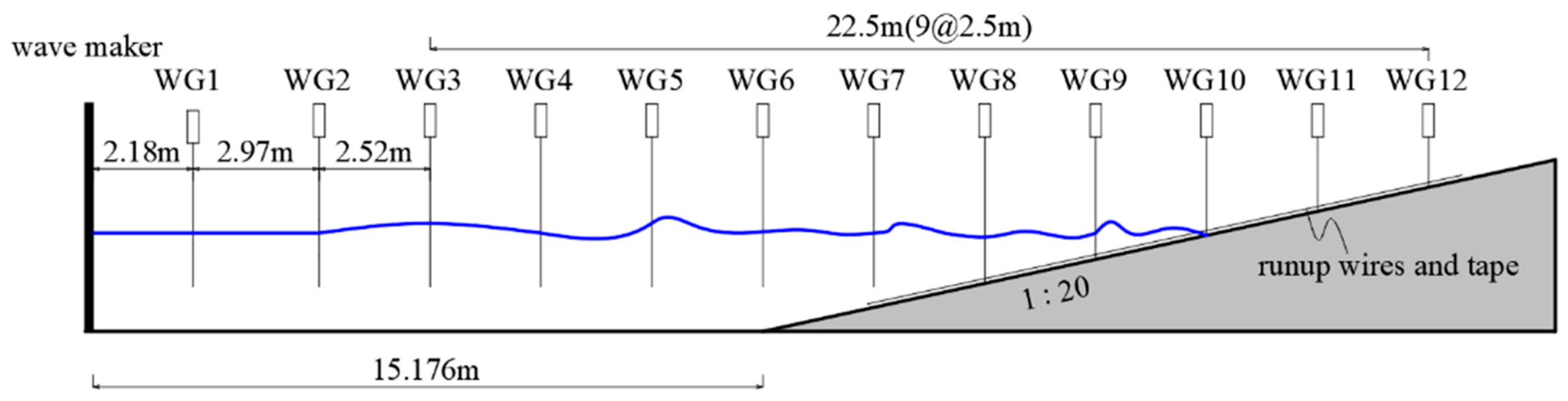
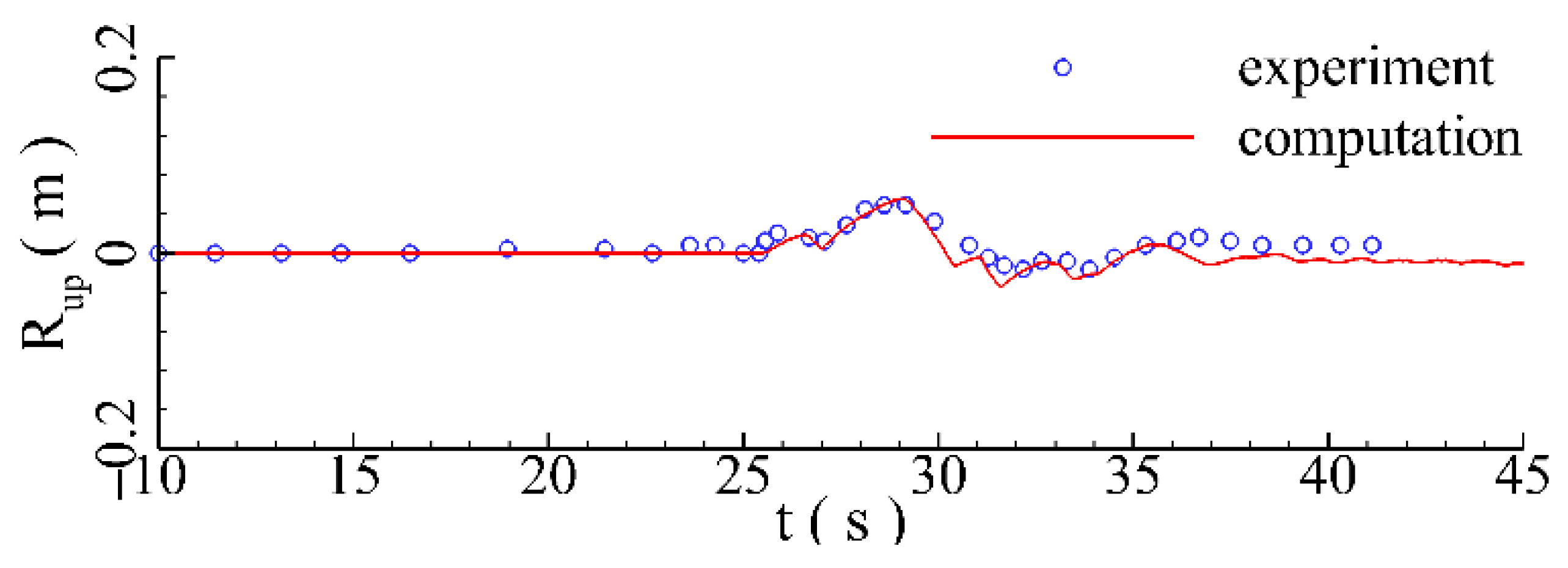
5.1. Transforming of Focused Wave Group on Sloped Beach

In this section, hydrodynamic processes of the wave generation and transformation of the focused wave group on a sloped beach are numerically simulated. The computed water elevations and wave runup height are validated by the experiment data [61]. Figure 1 shows the experimental layout. The experimental work was carried out in the laboratory flume located in COAST Laboratory at the Plymouth University, UK. The length and width of the wave flume is 35 m and 0.6 m, respectively. A 1:20 sloped beach was installed at the middle of the wave flume. The offshore water depth is 0.5 m. The sloped beach was located at 15.176 m from the wave paddle. Twelve resistance wave gauges were arranged along the flume at 2.5 m intervals to record the temporal and spatial variations of water elevations. The spacing between the first three wave gauges is different slightly, as depicted in Figure 1. The computational domain is also 35 m long. The focusing time ($t_f$) and location ($x_f$) are set as 30 s and 27.676 m. The grid resolution ($dx$) is kept as 0.01 m in the horizontal direction; 40 $\sigma$-grid layers are used in the vertical direction. Figure 2 shows the time series of water elevations at different wave gauges. Locations of the wave gauges are depicted in Figure 1. It is shown that the computed water elevations are in good agreements with the experiment data. Moreover, it is shown that the present nonhydrostatic flow solver can capture the hydrodynamic processes of the wave generation process in the offshore water region and the subsequent wave transformation on the sloped beach. The skill number proposed by Wilmott [73] is used to evaluate the degree of agreement between the predictions and experiment data. The skill numbers of water elevations at different wave height meters are greater overall than 0.83, verifying that the predicted water elevations match well with the measurements. Figure 3 depicts the temporal evolutions of wave runup height. As shown in Figure 3, the present nonhydrostatic flow solver can well capture the wave runup and descent on the sloped beach. The difference in the peak values for the wave runup height between the prediction and the experiment data is no more than 8%. As mentioned above, the computational capability of the present nonhydrostatic flow solver in predicting the hydrodynamics of a focused wave group has been well validated.

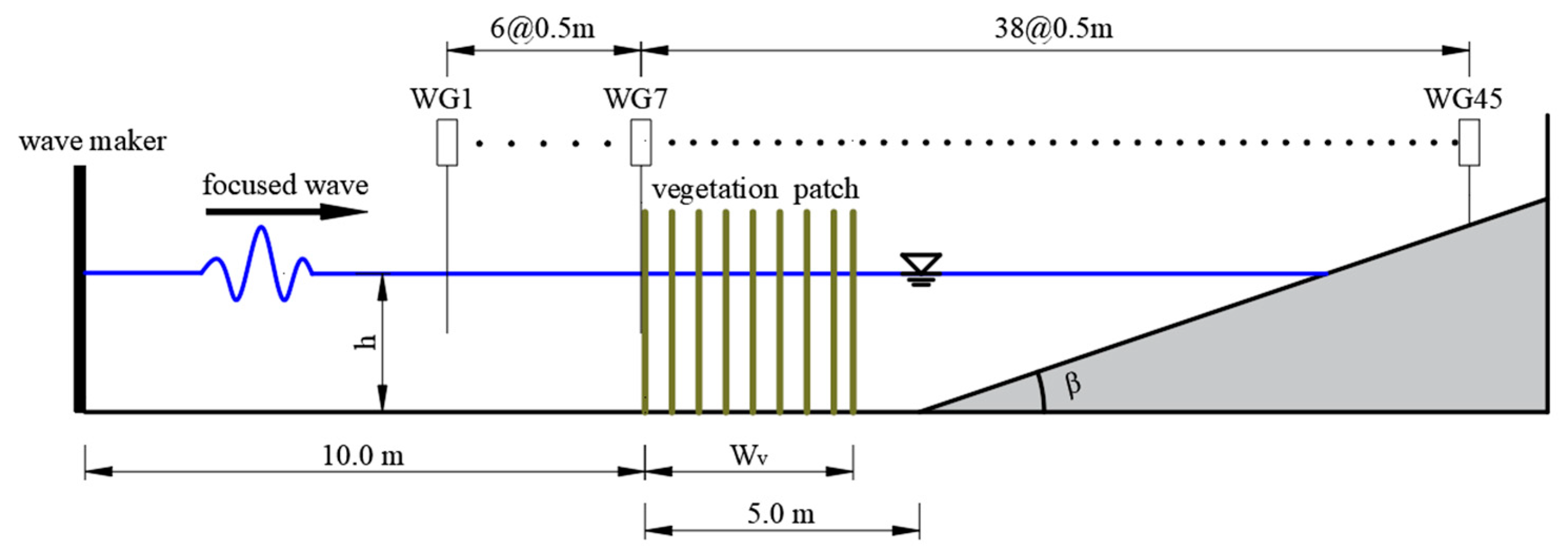
5.2. Regular Waves Propagating over Rigid Vegetation Patch

In this section, complicated interactions between the regular waves and emergent rigid vegetation patch are simulated by applying the present numerical wave model. The computed spatial distributions of wave heights are compared with the corresponding experiment data [74]. The physical experiment was carried out in a wave tank at the USDA-ARS National Sedimentation Laboratory (NSL) in Oxford. The experimental layout is depicted in Figure 4. The length and width of the wave flume are 20.6 m and 0.69 m, respectively. In the experiment, the front side of the emergent vegetation model was fixed at 11.5 m from the wave marker. The length of the vegetation patch was 3.66 m. The vegetation model was composed of a wooden cylinder, whose diameter is 9.5 mm. One wave gauge was installed at the front of vegetation patch to record the wave profile of incident waves. Four different wave gauges were laterally distributed along the vegetation patch to record the spatial variations of wave heights. Eight different experimental cases with different wave height, wave period, water depth, and vegetation density were chosen to validate the present nonhydrostatic flow solver. The parameter setups for these eight experimental cases are listed in

Table 1. Parameter setups for different experimental cases.

Case	$\mathit{h}$ (m)	$\mathit{T} \left(\mathbf{s}\right)$	$\mathit{H} \left(\mathbf{m}\right)$	${\mathit{N}}_{\mathit{v}} \left(\mathbf{stem}/{\mathbf{m}}^2\right)$
1	0.5	0.7	0.053	350
2	0.5	0.7	0.053	623
3	0.5	1.0	0.1	350
4	0.5	1.0	0.1	623
5	0.7	1.2	0.052	350
6	0.7	1.2	0.052	623
7	0.7	1.1	0.117	350
8	0.7	1.1	0.117	623

. The length of computational domain is 20 m. The grid resolution ($dx$) is 0.01 m in the horizontal direction. In the vertical direction, 40 $\sigma$-mesh layers are applied. As suggested by Jiang et al. [75] and Qu et al. [63], the drag coefficient ($C_D$) is set as 1.2 for all computational runs. Figure 5 depicts the spatial distributions of the averaged wave heights under different parameter setups. It is seen that the predicted averaged wave height within the vegetation path match well with the experiment data. The skill number proposed by Willmott [73] is used to evaluate the degree of agreement between the predictions and experiment data. All the skill numbers of averaged wave height under all parameter setups are greater than 0.86, indicating that the computational capability of present numerical wave model is reliable and the chosen drag coefficient ($C_D$) is accurate.

6. Discussions on Results

Influences of the emergent rigid vegetation patch on the runup processes of the focused wave groups are numerically investigated in the following sections. Effects of the major factors, i.e., water depth ($h$), peak wave period ($T_p$), significant wave height ($H_s$), and density ($N_v$), and length ($W_v$) of vegetation patch are discussed in detail. As in Section 5.2, the drag coefficient ($C_D$) is set as 1.2 for all computational runs. The computational layout is plotted in Figure 6. The front side of the vegetation patch is fixed at 10 m from the inlet. The slope beach is located 15 m away from the inlet.

Table 2. Parameter setups for different simulation runs.

Run	${\mathit{H}}_{\mathit{s}} \left(\mathbf{m}\right)$	$\mathit{h} \left(\mathbf{m}\right)$	${\mathit{T}}_{\mathit{p}} \left(\mathit{s}\right)$	$\mathit{t}\mathit{a}\mathit{n}\mathit{\beta }$	${\mathit{N}}_{\mathit{v}} \left(\mathbf{stem}/{\mathbf{m}}^2\right)$	${\mathit{W}}_{\mathit{v}} \left(\mathbf{m}\right)$
1	0.05	0.5	1.2	1:20	350	3.5
2	0.075	0.5	1.2	1:20	350	3.5
3	0.1	0.5	1.2	1:20	350	3.5
4	0.125	0.5	1.2	1:20	350	3.5
5	0.1	0.4	1.2	1:20	350	3.5
6	0.1	0.6	1.2	1:20	350	3.5
7	0.1	0.7	1.2	1:20	350	3.5
8	0.1	0.5	1.5	1:20	350	3.5
9	0.1	0.5	1.8	1:20	350	3.5
10	0.1	0.5	2.1	1:20	350	3.5
11	0.1	0.5	1.2	1:5	350	3.5
12	0.1	0.5	1.2	1:10	350	3.5
13	0.1	0.5	1.2	1:15	350	3.5
14	0.1	0.5	1.2	1:25	350	3.5
15	0.1	0.5	1.2	1:20	450	3.5
16	0.1	0.5	1.2	1:20	550	3.5
17	0.1	0.5	1.2	1:20	650	3.5
18	0.1	0.5	1.2	1:20	350	2.5
19	0.1	0.5	1.2	1:20	350	3
20	0.1	0.5	1.2	1:20	350	4
21	0.1	0.5	1.2	1:20	350	4.5
22	0.1	0.5	1.2	1:20	350	5

lists the parameter setups for different simulation runs. For the basic run (Run 3 in the Table 2), the density ($N_v$) and the length ($W_v$) of the vegetation patch is 350 stem/m² and 3.5 m, respectively. Meanwhile, water depth ($h$) is 0.5 m, significant wave height ($H_s$) is 0.1 m, peak wave period ($T_p$) is 1.2 s, and slope of the beach ($tan\beta$) is 1:20.

6.1. Hydrodynamic Phenomena

Complicated interactions between the focused wave group and the emergent vegetation patch and the influences of the emergent vegetation patch on the runup processes of the focused wave group are discussed in this section. Snapshots of the water velocity contours at different time moments are plotted in Figure 7. When the wave components with different wave parameters enter the computational domain, the wave profile of the focused wave group is to evolve (Figure 7a,g). High-velocity water region can be found near the peak wave crest. The incident waves are designed to focus on the front side of the vegetation patch (Figure 7b,h). Attributed to the wave attenuation effects of the vegetation patch, the peak wave crest can be significantly reduced, compared with the focused wave group without the vegetation patch (Figure 7c,i). Meanwhile, the velocity magnitude of the water body can be also greatly decreased. After the transmitted wave group leaves the vegetation patch (Figure 7d,e), the reshaped wave group is run up along the sloped beach and finally results in a lower maximum wave runup height (Figure 7f).

Figure 8 plots the water elevations at the front and rear sides of the emergent rigid vegetation patch. As depicted in Figure 8, the incident waves focus on front side of the vegetation patch for both focused wave groups with and without the emergent rigid vegetation patch. Due to the existence of vegetation patch, peak value of the water elevation of the focused wave group can be greatly reduced (about 28.1%), compared with the focused wave group without the emergent rigid vegetation patch. The spatial distribution of the local maximum wave height within the vegetation patch are plotted in Figure 9, where the local wave height represents the local wave crest minus wave trough. It clearly shows that when the focused wave group propagates within the vegetation patch, the maximum local wave height can be greatly reduced due to the combined effect of the damping effects of emergent vegetation and the bottom friction. Moreover, damping effects of the vegetation patch become dominant in reducing the local wave height of focused wave group. The maximum local wave height of focused wave group can be reduced 31.2% by the vegetation patch, compared with the focused wave group without the vegetation patch at the rear side of the vegetation patch.

Figure 10 plots the energy fluxes at the front and rear sides of the vegetation patch. Although the temporal evolutions of energy fluxes of the focused wave group with and without the vegetation patch coincide with each other at the front side of the vegetation patch, the peak value of the energy flux of the focused wave group with vegetation patch is much lower than that without the vegetation patch at the rear side of the vegetation patch (57.3% lower), indicating the wave attenuation capability of the vegetation patch. Figure 11 depicts the time series of the different kinds of water wave energies during the runup processes of focused wave groups. It is shown that once the incident waves enter the computational domain, water wave energies gradually increase. At $t$ = 10 s, the kinetic energy, potential energy, and the corresponding total wave energy of the water body approach their maximum values. When the focused wave group propagates across the emergent vegetation patch (15 < $t$ < 20 s), attributed to the significant wave damping effects of the vegetation patch, the kinetic energy, potential energy, and total wave energy of the water body can be reduced by 48.5%, 56.5%, and 51.1%, respectively, compared with the focused wave group without the vegetation patch.

Figure 12 plots the time series of the wave runup height for the focused wave group with and without the vegetation patch. As depicted in Figure 12, the temporal evolution of the wave run height is basically consistent with the temporal evolution of the focused wave profile. Attributed to the wave damping effects of the vegetation patch, the maximum value of the wave runup height of the focused wave group with the vegetation patch is about 22.0% lower than that without the vegetation patch. This further illustrates the damping effects of the emergent vegetation patch on the runup processes of the focused wave group. Through the above analysis, it is shown that the existence of the emergent vegetation patch has great effects on the hydrodynamics of wave runup processes of a focused wave group on the sloped beach. The presence of a vegetation patch can greatly reduce the wave runup height of extreme waves and effectively protect the coast.

6.2. Effects of Significant Wave Height

This section discusses the influences of the emergent vegetation patch on the runup processes of focused wave groups under different significant wave heights. Figure 13 depicts the spatial distributions of local maximum wave height within the vegetation patch under different significant wave heights. When the vegetation patch is absent, the local maximum wave height of the focused wave group can only slightly decrease because of the bottom friction and the wave profile evolutions. Once the vegetation patch is present, the local maximum wave height of the focused wave group will be significantly decreased. Moreover, difference between the local maximum wave height between the focused wave groups with and without the vegetation at the rear side of the vegetation patch gradually increases with the significant wave height. Figure 14 depicts the variation in decreasing rate of the local maximum wave height at the rear side of the vegetation patch with the significant wave height. It clearly shows that the decreasing rate of the local maximum wave height linearly increases with the significant wave height. As the relative wave height ($H_s/h$) increases from 0.1 to 0.25, decreasing rate of the local maximum wave height increase by 19.0%. Figure 15 depicts the variation in wave energy dissipation rate with the significant wave height. When the incident waves propagate within the vegetation patch, most of the incident wave energy can be dissipated. Wave energy dissipation rate gradually increases with the significant wave height. When the relative wave height ($H_s/h$) increases gradually from 0.1 to 0.25, the wave energy dissipation rate increases by 25.6%. Figure 16 depicts the variation in maximum wave runup height with the significant wave height. Maximum wave runup height almost increases linearly with the significant wave height. Since the presence of the vegetation patch can dissipate a great portion of the incident wave energy, the maximum values for the wave runup height of the focused wave group with the vegetation patch are smaller, 25% smaller on average, than that without the vegetation patch.

6.3. Effects of Water Depth

Influences of the emergent vegetation patch on the runup processes of focused wave groups under different water depths are presented in this section. Figure 17 shows the spatial distribution of local maximum wave height within the vegetation patch. Because of the frictional force at the bottom and the wave evolution process, the local maximum wave height of the focused wave group without the vegetation can only slightly decrease along the vegetation patch. When the vegetation patch is present, the local maximum wave height will decrease obviously when the focused wave group propagates within the vegetation patch. However, the decreasing rate of the local maximum wave height gradually slows down with the increasing of water depth. Figure 18 plots the variation in the decreasing rate of the local maximum wave height at rear side of the vegetation patch. As shown in Figure 18, the decreasing rate of the local maximum wave height only slightly decreases in a linear mode with the water depth. As the water depth ($h$) increases from 0.4 m to 0.7 m, decreasing rate of the local maximum wave height at rear side of the vegetation patch can only decrease by 2.8%. The variation in the wave energy dissipation rate with the water depth is plotted in Figure 19. When the water depth is less than 0.5 m, the dissipation rate of the wave energy is almost a constant and can only be slightly influenced by the water depth. Once the water depth ($h$) is greater than 0.5 m, the dissipation rate of the wave energy sharply decreases with the water depth at a high rate. As the water depth ($h$) gradually increases from 0.5 m to 0.7 m, the dissipation rate of the wave energy decreased by 23.5%. In the case of a given significant wave height, the increase in the water depth will increase the effective wavelength of the incident waves, which will lead to a gradual decrease in the magnitude of wave-induced water velocity. Finally, the energy dissipation rate is decreased. Figure 20 shows the variation in maximum wave runup height with the water depth. Given the significant wave height $H_s$ = 0.1 m, the maximum wave runup height can only slightly decrease with the water depth. As the water depth ($h$) gradually increases from 0.4 m to 0.7 m, the maximum wave runup height of the focused wave group with and without the vegetation patch can be decreased by 22.6% and 22.0%, respectively. Attributed to the damping effects of the emergent vegetation patch, maximum wave runup height of the focused wave group with the vegetation patch are always smaller than that without the vegetation patch, 21.5% smaller on average, under different water depths.

6.4. Effects of Peak Wave Period

This section analyzes the influences of the peak wave period on the wave attenuation of focused wave groups by the emergent vegetation patch. Figure 21 shows the spatial distributions of the local maximum wave height within the vegetation patch. Apparently, the local maximum wave height of the focused wave group tends to decrease along the emergent vegetation patch. Due to the extra drag force of the emergent vegetation patch, local maximum wave height of the focused wave group with the vegetation patch is always smaller than that without the vegetation patch. However, differences in the local maximum wave height of focused wave groups with and without the vegetation patch tend to decrease with the peak wave period. Figure 22 shows the variation in the decreasing rate of the local maximum wave height at the rear side of the vegetation patch with the peak wave period. As depicted in Figure 22, the decreasing rate of the local maximum wave height monotonically decreases with the peak wave period. As the peak wave period ($T_p$) gradually increases from 1.2 s to 2.1 s, decreasing rate of the local maximum wave height decreases by 12.8%. Given the significant wave height and water depth, the increase in peak wave period will enlarge the effective wavelength of incident wave components, resulting in a gradual decreasing in the magnitude of wave-induced water velocity. Hence, the energy dissipation rate decreases with the peak wave period, as depicted in Figure 23. As the peak wave period ($T_p$) increases from 1.2 s to 2.1 s, the wave energy dissipation rate of the focused wave group with the vegetation patch decreases by 9.2%. As depicted in Figure 24, the maximum wave runup height monotonically increases with the peak wave period. As the peak wave period ($T_p$) increases from 1.2 s to 2.1 s, the maximum wave runup height of the focused wave group with and without the vegetation patch increases by 40.1% and 45.6%, respectively. Attributed to the damping effects of the emergent vegetation patch, maximum wave runup height of the focused wave group with the vegetation patch are always smaller than that without the vegetation patch, 23.6% smaller on average, under different peak wave periods.

6.5. Effects of Vegetation Density

This section analyzes the influences of vegetation density on the wave runup of focused wave groups. Figure 25 shows the spatial distributions of the local maximum wave height within the vegetation patch under different vegetation densities. Attributed to the wave attenuation of the emergent vegetation patch, the local maximum wave height of the focused wave group with the vegetation patch tends to decrease along the vegetation patch. Since a higher vegetation density can enhance the wave damping effects of the vegetation patch, differences in the local maximum wave height of focused wave groups with and without the vegetation patch tend to increase with the vegetation patch. Figure 26 shows the variation in the decreasing rate of local maximum wave height at the rear side of vegetation patch. As seen in Figure 26, the decreasing rate of the local maximum wave height monotonically increases with the vegetation density. When the vegetation density ($N_v$) increases from 350 stem/m² to 650 stem/m², the decreasing rate of the local maximum wave height increases by 14.4%. The increase in vegetation density will enhance the ability of the vegetation patch to damp the incident waves. As a result, the wave energy dissipation rate monotonically increases with the vegetation density, as depicted in Figure 27. When the vegetation density ($N_v$) increases from 350 stem/m² to 650 stem/m², the wave energy dissipation rate of the focused wave group with the vegetation patch increases by 18.0%. Figure 28 plots the variation in maximum wave runup height with the vegetation density. Apparently, the maximum wave runup height monotonically decreases with the vegetation density. When the vegetation density ($N_v$) increases from 350 stem/m² to 650 stem/m², the maximum wave runup height of the focused wave group with the vegetation patch decreases by 13.7%.

6.6. Effects of Vegetation Length

This section analyzes the influences of vegetation length on the wave runup of focused wave groups. Figure 29 shows the water velocity contours under different vegetation lengths. With the increase in vegetation length, velocity magnitude of the water body decreases significantly after the focused wave group leaving the vegetation patch. Figure 30 depicts the spatial distribution of the local maximum wave height within the vegetation patch under different vegetation lengths. As shown in Figure 30, the local maximum wave height of the focused wave group tends to gradually decrease along the vegetation patch under different vegetation lengths. Attributed to the extra drag force of the vegetation patch, the local maximum wave height of the focused wave group with the vegetation patch is always smaller than that without the emergent vegetation patch. At the same time, differences in the local maximum wave height of the focused wave groups with and without the vegetation patch gradually tend to increase with the length of vegetation patch. Figure 31 shows the variation in the decreasing rate of the local maximum wave height at the rear side of the vegetation patch with the vegetation length. As shown in Figure 31, the decreasing rate of the local maximum wave height monotonically increases with the vegetation length. When the vegetation length ($W_v$) increases from 2.5 m to 5 m, the decreasing rate of the local maximum wave height increases by 13.1%. Figure 32 shows the variation in wave energy dissipation rate with the vegetation length. Obviously, the wider the vegetation patch, the more the wave energy can be dissipated when the focused wave group passes through the vegetation patch. As the peak wave period ($W_v$) increases from 2.5 m to 5 m, wave energy dissipation rate of the focused wave group by the vegetation patch increases by 18.0%. Figure 33 shows the variations in maximum wave runup height with the vegetation length. As depicted in Figure 33, maximum wave runup height decreases monotonically with the vegetation length. When the vegetation length ($W_v$) increases from 2.5 m to 5 m, maximum wave runup height of the focused wave group with the vegetation patch decreases by 12.8%.

7. Conclusions

In this study, influences of the emergent vegetation patch on the runup processes of focused waves were investigated by applying a nonhydrostatic flow solver (NHWAVE). Effects of the major factors, i.e., water depth, peak wave period, significant wave height, and density and length of the vegetation patch, are analyzed in detail. The main findings are organized as follows:

(1)

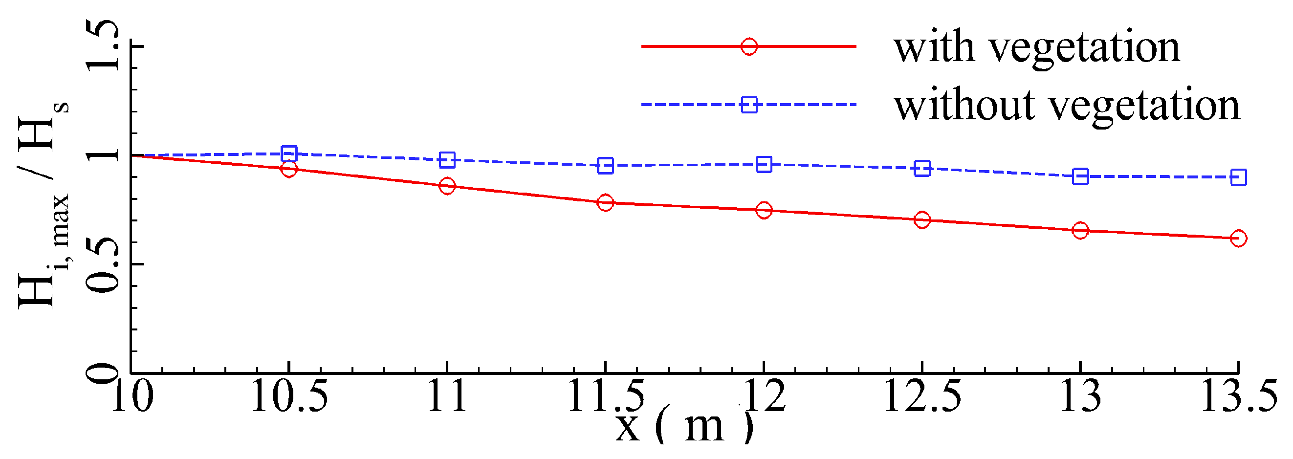
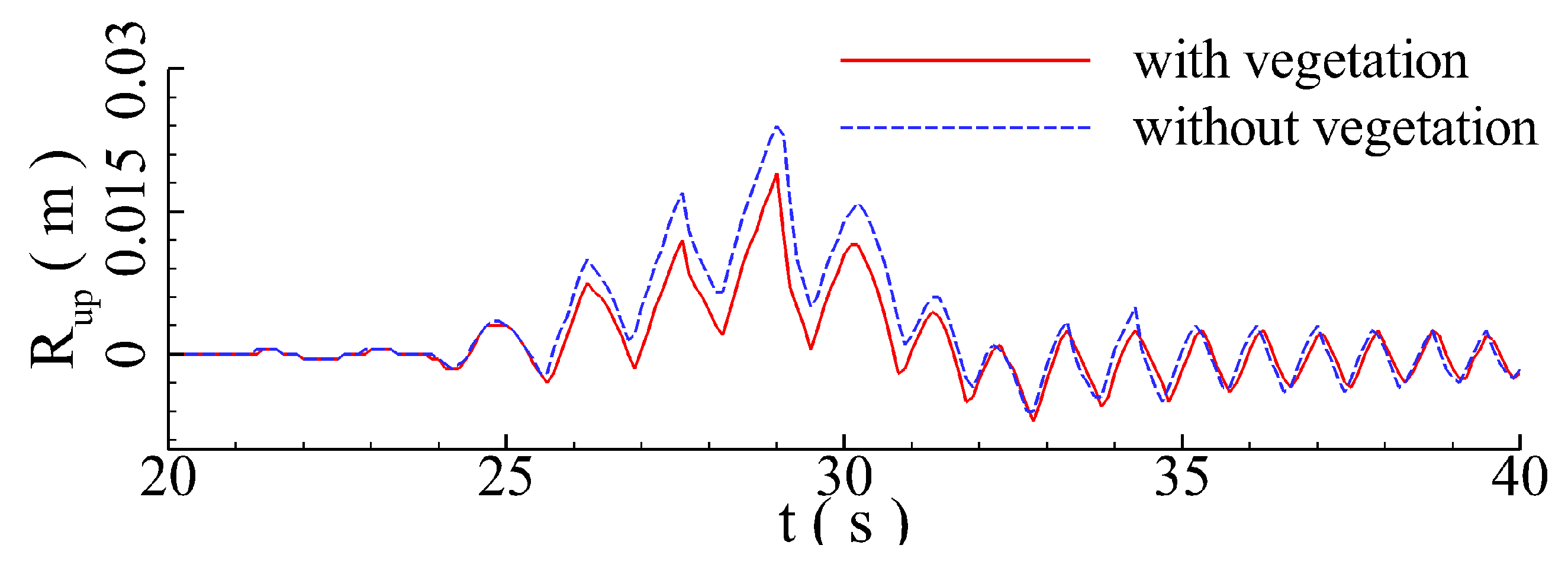
As the focused wave group propagates across the emergent vegetation patch, kinetic energy, potential energy, and total wave energy of the water body can be reduced by 48.5%, 56.5%, and 51.1%, respectively. The maximum value for the wave runup height of a focused wave group with the vegetation patch is about 22% lower than that without the vegetation patch. Hence, the presence of a vegetation patch can greatly reduce the wave runup height of extreme waves and effectively protect the coast.

(2)

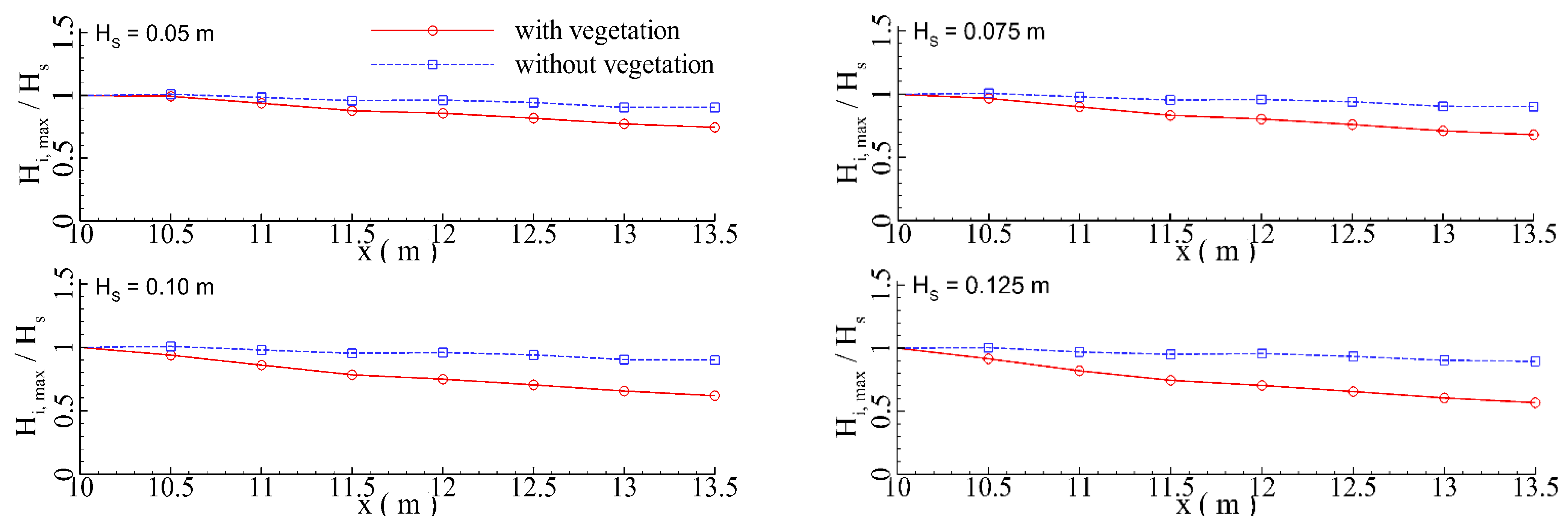
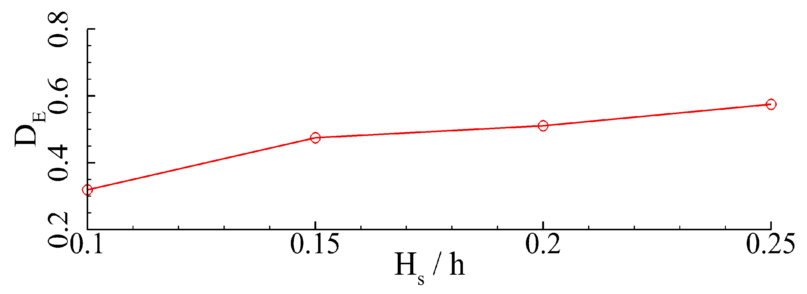
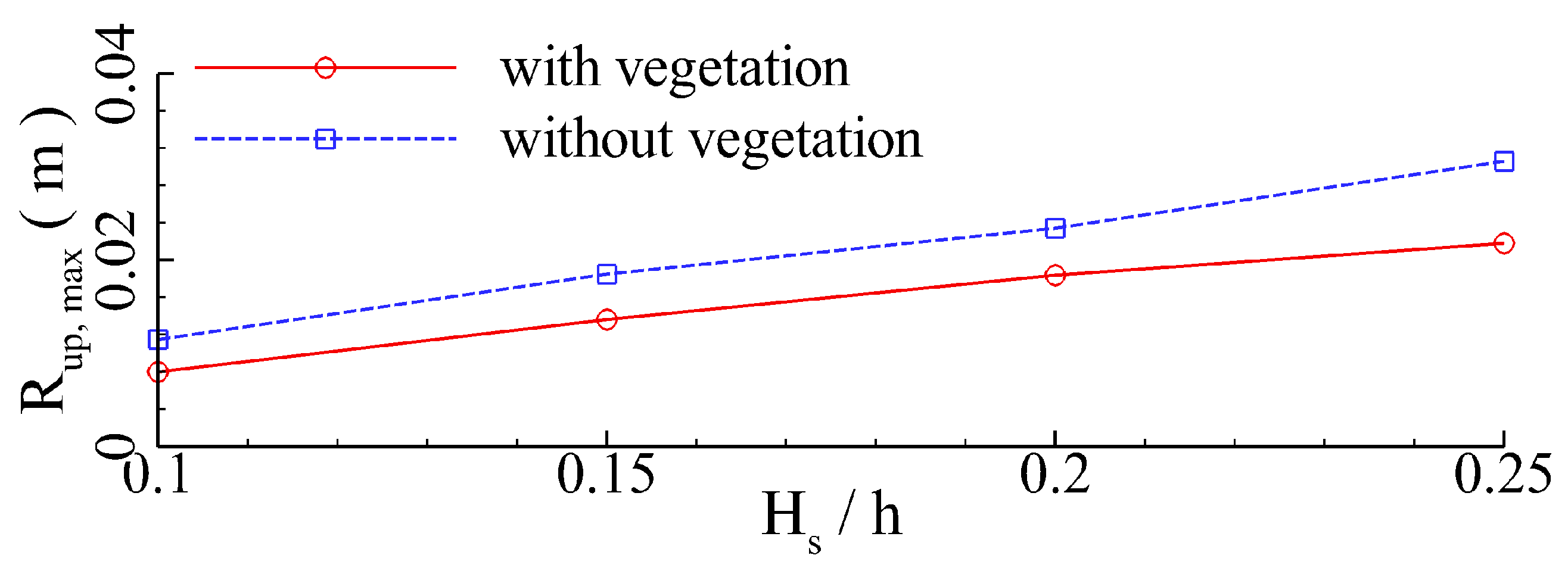
Wave energy dissipation rate gradually increases with significant wave height. As the relative significant wave height increases from 0.1 to 0.25, the wave energy dissipation rate can increase by 25.6%. The presence of the vegetation patch can dissipate a great portion of the incident wave energy. Therefore, maximum values for the wave runup height of a focused wave group with the vegetation patch are always smaller, 25% smaller on average, than that without the vegetation patch.

(3)

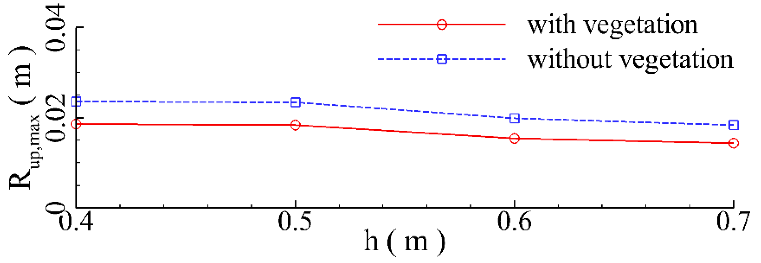
Given the specific significant wave height, the increase in the water depth will increase the effective wavelength of the incident waves, which will lead to a gradual decrease in the magnitude of wave-induced water velocity. Then, the energy dissipation rate decreases. Hence, the maximum wave runup height tends to slightly decrease with the water depth. As the water depth increases from 0.4 to 0.7 m, the maximum wave runup height of the focused wave group with and without the vegetation patch can be decreased by 22.6% and 22%, respectively.

(4)

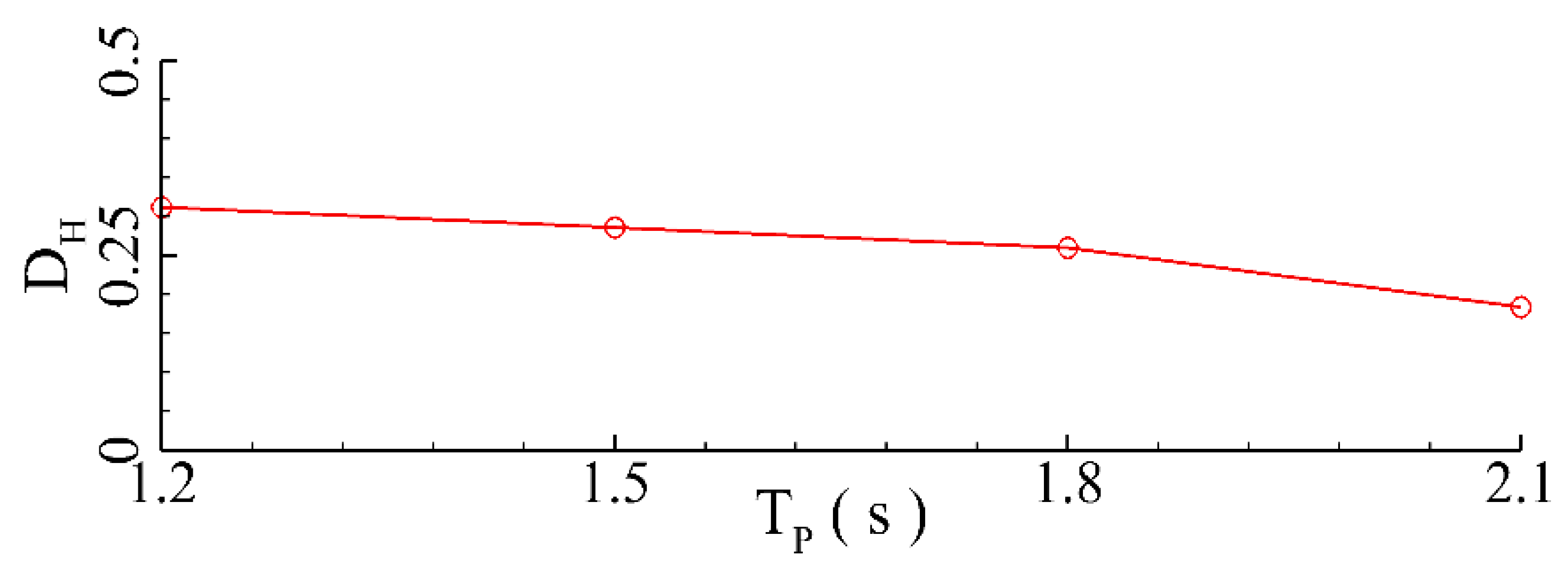
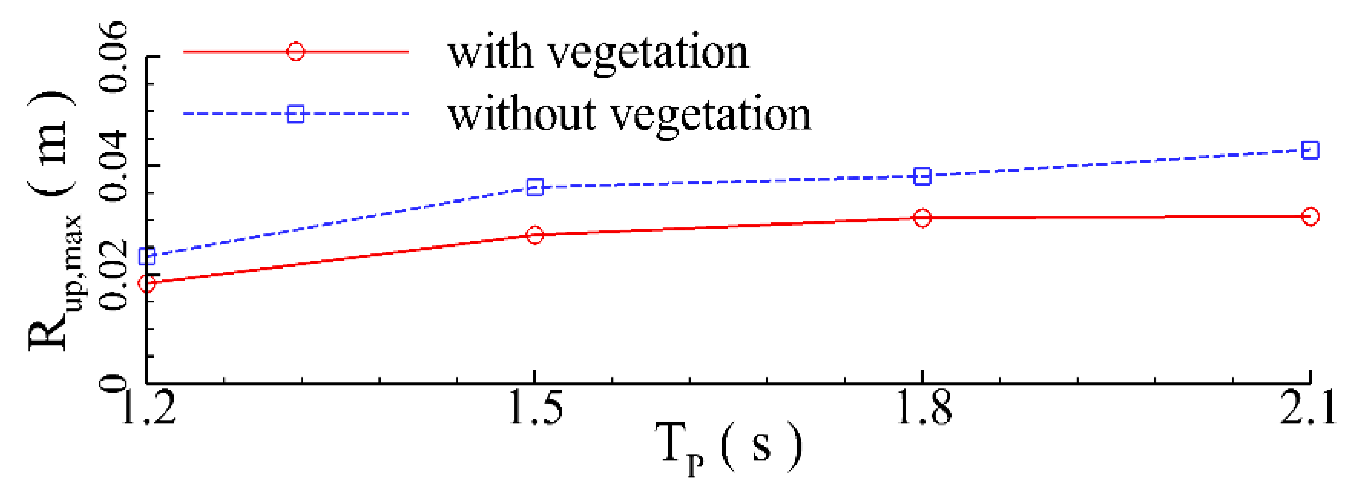
Since the increase in peak wave period can increase the effective wavelength of the incident wave components, magnitude of the wave-induced water velocity gradually decreases. Therefore, wave energy dissipation rate gradually decreases with the peak wave period, and the maximum wave runup height monotonically increases with the peak wave period. When the peak wave period increases from 1.2 s to 2.1 s, the maximum wave runup height of the focused wave group with and without the vegetation patch increases by 40.1% and 45.6%, respectively.

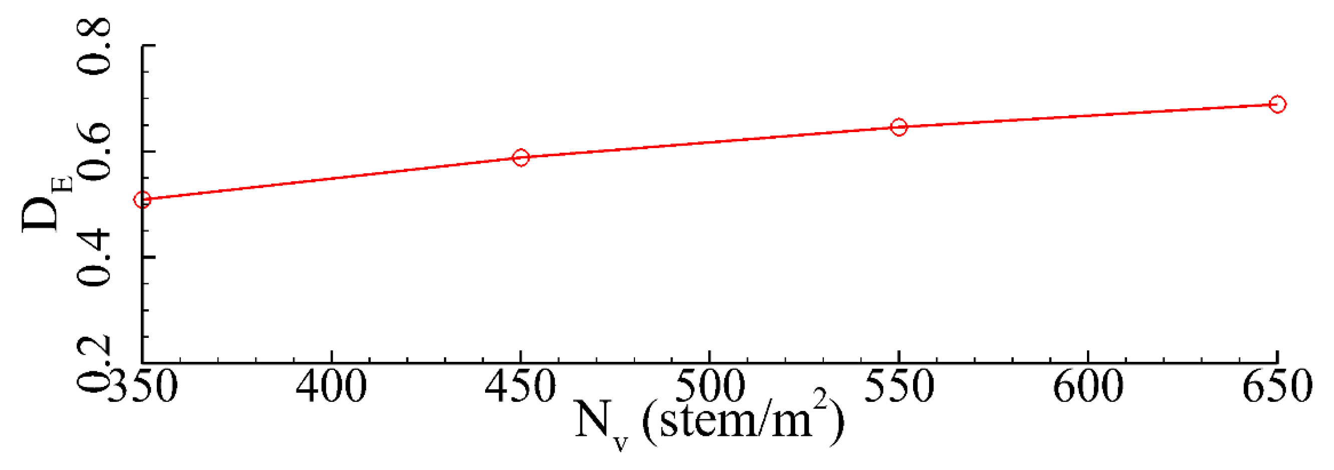
(5)

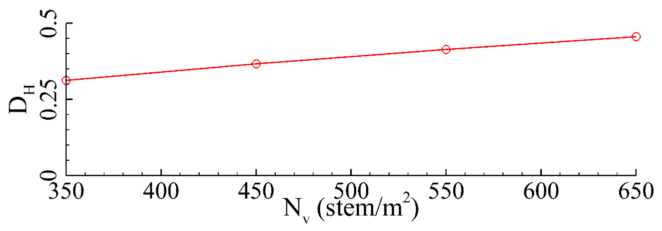
Since a higher vegetation density can enhance the wave damping effects of the vegetation patch, as the vegetation density increases from 350 stem/m² to 650 stem/m², the maximum wave runup height of the focused wave group with the vegetation patch decreases by 13.7%.

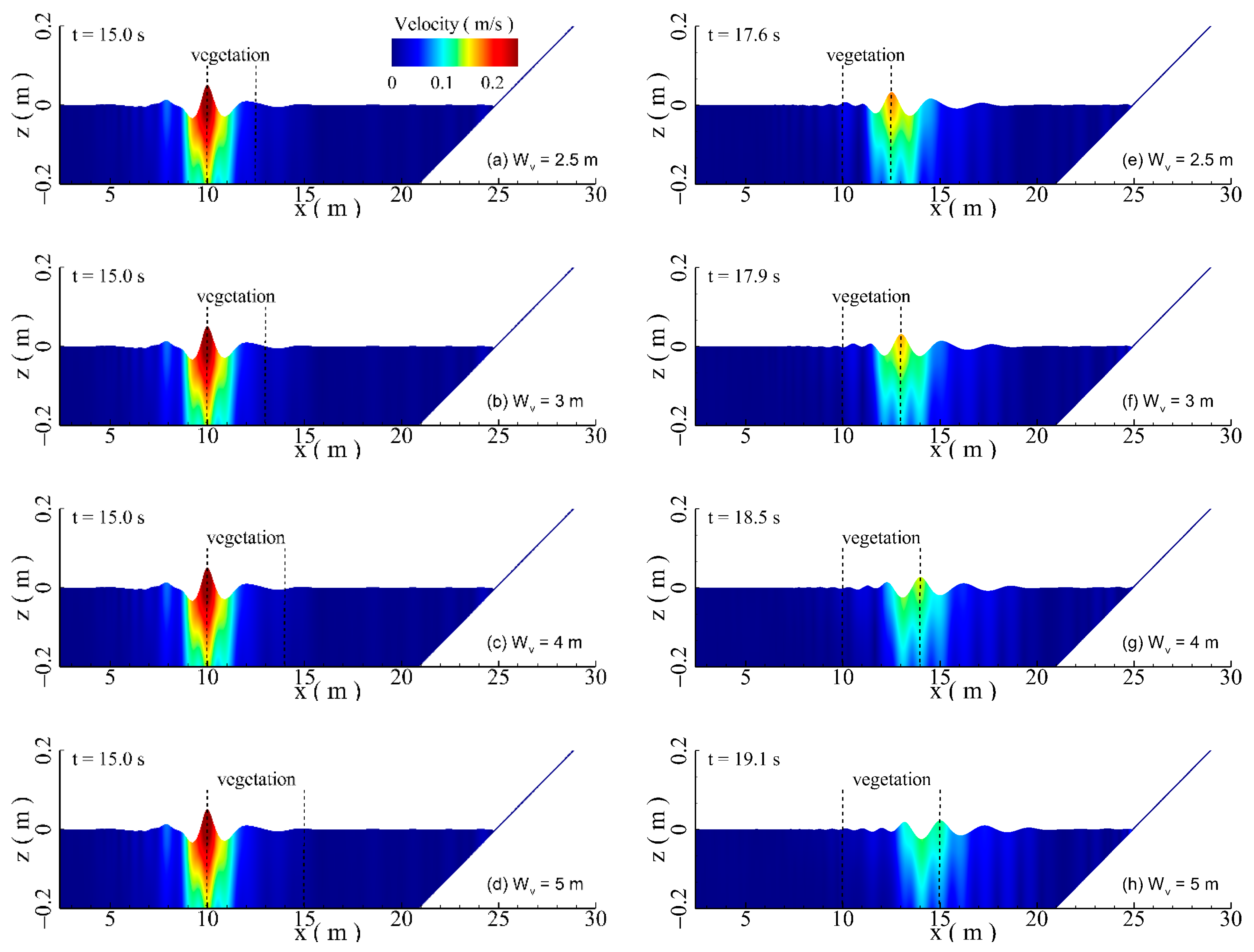
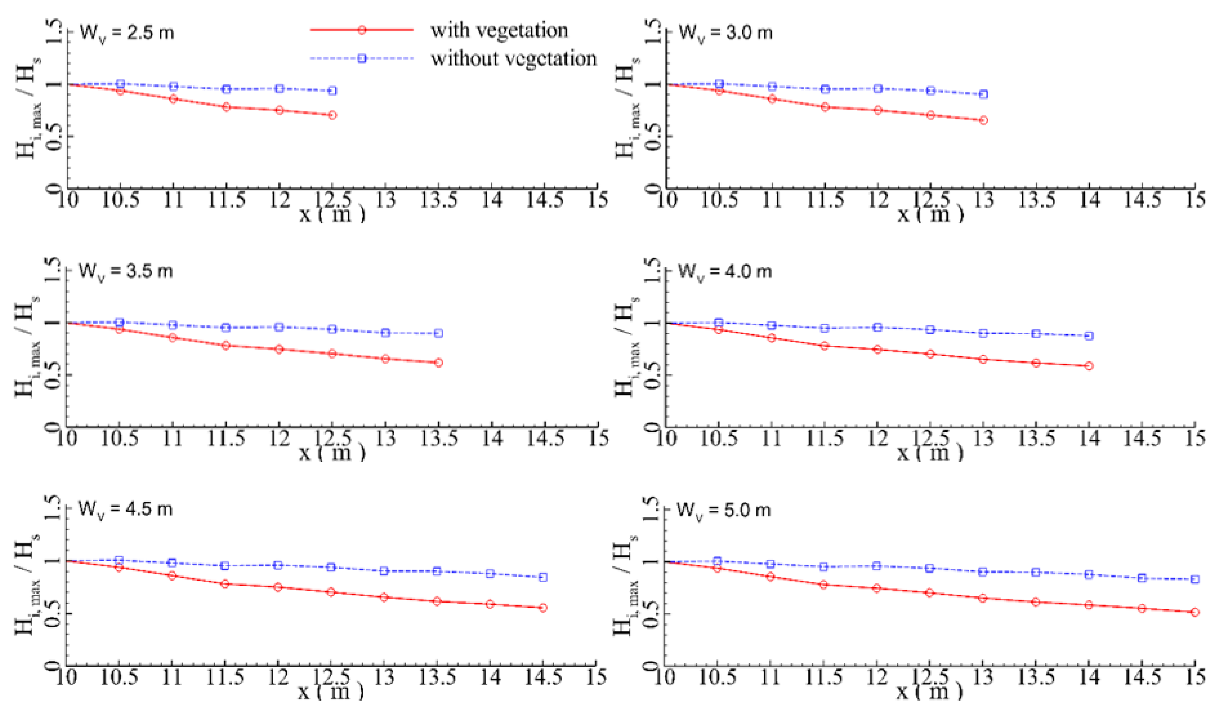
(6)

The maximum wave runup height monotonically decreases with the vegetation length. When the vegetation length increases from 2.5 m to 5 m, the maximum wave runup height of the focused wave group with the vegetation patch decreases by 12.8%.

It is expected that the present research results will have some reference significance for the design of coastal soft protection measures.

References

- Mori, N.; Takahashi, T.; Yasuda, T.; Yanagisawa, H. Survey of 2011 Tohoku earthquake tsunami inundation and run-up. Geophys. Res. Lett. 2011, 38, L00G14. [Google Scholar] [CrossRef]
- Jongman, B.; Hochrainer-Stigle, S.; Feyen, L.; Aerts, J.C.J.H.; Mechler, R.; Botzen, W.J.W.; Bouwer, L.M.; Pflug, G.; Rojas, R.; Ward, P.J. Increasing stress on disaster-risk finance due to large floods. Nat. Clim. Chang. 2014, 4, 264–268. [Google Scholar] [CrossRef]
- Qu, K.; Yao, W.; Tang, H.S.; Agrawal, A.; Shields, G.; Chien, S.I.; Gurung, S.; Imam, Y.; Chiodi, I. Extreme storm surges and waves and vulnerability of coastal bridges in New York City metropolitan region: An assessment based on Hurricane Sandy. Nat. Hazards 2021, 105, 2697–2734. [Google Scholar] [CrossRef]
- Maza, M.; Lara, J.L.; Losada, I.J. Experimental analysis of wave attenuation and drag forces in a realistic fringe Rhizophora mangrove forest. Adv. Water. Resour. 2019, 131, 103376. [Google Scholar] [CrossRef]
- Chang, C.W.; Mori, N. Green infrastructure for the reduction of coastal disasters: A review of the protective role of coastal forests against tsunami, storm surge, and wind waves. Coast. Eng. J. 2021, 63, 370–385. [Google Scholar] [CrossRef]
- Knutson, P.L.; Brochu, R.A.; Seelig, W.; Inskeep, M. Wave damping in spartina alterniflora marshes. Wetlands 1982, 2, 87–104. [Google Scholar] [CrossRef]
- Yang, S.L.; Shi, B.W.; Bouma, T.J. Wave attenuation at a salt marsh margin: A case study of an exposed coast on the yangtze estuary. Estuar. Coasts 2012, 35, 169–182. [Google Scholar] [CrossRef]
- Qu, K.; Lan, G.Y.; Kraatz, S.; Sun, W.Y.; Deng, B.; Jiang, C.B. Numerical study on wave attenuation of tsunami-like wave by emergent rigid vegetation. J. Earthq. Tsunami 2021, 15, 2150028. [Google Scholar] [CrossRef]
- Sun, W.Y.; Qu, K.; Kraatz, S.; Lan, G.Y.; Jiang, C.B. Numerical investigation of the attenuation of tsunami-like waves by a vegetated, sloped Beach. J. Earthq. Tsunami 2022, 16, 2140008. [Google Scholar] [CrossRef]
- Kathiresan, K.; Rajendran, N. Coastal mangrove forests mitigated tsunami. Estuar. Coast. Shelf Sci. 2005, 65, 601–606. [Google Scholar] [CrossRef]
- Bao, T.Q. Effect of mangrove forest structures on wave attenuation in coastal Vietnam. Oceanologia 2011, 53, 807–818. [Google Scholar]
- Jadhav, R.S.; Chen, Q.; Smith, J.M. Spectral distribution of wave energy dissipation by salt marsh vegetation. Coast. Eng. 2013, 77, 99–107. [Google Scholar] [CrossRef]
- Lee, W.K.; Tay, S.H.X.; Ooi, S.K.; Friess, D.A. Potential short wave attenuation function of disturbed mangroves. Estuar. Coast. Shelf Sci. 2021, 248, 106747. [Google Scholar] [CrossRef]
- Rozas, L.P.; Odum, W.E. Occupation of submerged aquatic vegetation by fishes: Testing the roles of food and refuge. Oecologia 1988, 77, 101–106. [Google Scholar] [CrossRef]
- Furukawa, K.; Wolanski, E.; Mueller, H. Currents and sediment transport in mangrove forests. Estuar. Coast. Shelf. Sci. 1997, 44, 301–310. [Google Scholar] [CrossRef]
- Hansen, J.C.R.; Reidenbach, M.A. Wave and tidally driven flows in eelgrass beds and their effect on sediment suspension. Mar. Ecol. Prog. Ser. 2012, 448, 271–288. [Google Scholar] [CrossRef]
- Manca, E.; Cáceres, I.; Alsina, J.M.; Stratigki, V.; Townend, I.; Amos, C.L. Wave energy and wave-induced flow reduction by full-scale model Posidonia oceanica seagrass. Cont. Shelf. Res. 2012, 50–51, 100–116. [Google Scholar] [CrossRef]
- Dalrymple, R.A.; Kirby, J.T.; Hwang, P.A. Wave diffraction due to areas of energy dissipation. J. Waterw. Port Coast. Ocean Eng. 1984, 110, 67–79. [Google Scholar] [CrossRef]
- Larson, M. Model for decay of random waves in surf zone. J. Waterw. Port Coast. Ocean Eng. 1995, 121, 1–12. [Google Scholar] [CrossRef]
- Hu, Z.; Suzuki, T.; Zitman, T.; Unittewaal, W.; Stive, M. Laboratory study on wave dissipation by vegetation in combined current-wave flow. Coast. Eng. 2014, 88, 131–142. [Google Scholar] [CrossRef]
- Hu, Z.; Borsje, B.W.; van Belzen, J.; Willemsen, P.W.J.M.; Wang, H.; Peng, Y.; Yuan, L.; De Dominicis, M.; Wolf, J.; Temmerman, S.; et al. Mechanistic modelling of marsh seedling establishment provides a positive outlook for coastal wetland restoration under global climate change. Geophys. Res. Lett. 2015, 48, e2021GL095596. [Google Scholar]
- Huang, Z.; Yu, Y.; Sim, S.Y.; Yao, Y. Interaction of solitary waves with emergent, rigid vegetation. Ocean Eng. 2011, 38, 1080–1088. [Google Scholar] [CrossRef]
- Iimura, K.; Tanaka, N. Numerical simulation estimating effects of tree density distribution in coastal forest on tsunami mitigation. Ocean Eng. 2012, 54, 223–232. [Google Scholar] [CrossRef]
- Maza, M.; Lara, J.L.; Losada, I.J. Tsunami wave interaction with mangrove forests: A 3-d numerical approach. Coast. Eng. 2015, 98, 33–54. [Google Scholar] [CrossRef]
- Möeller, I. Quantifying saltmarsh vegetation and its effect on wave height dissipation: Results from a UK east coast saltmarsh. Estuar. Coast. Shelf Sci. 2006, 69, 337–351. [Google Scholar] [CrossRef]
- Twomey, A.J.; O’Brien, K.R.; Callaghan, D.P.; Saunders, M.I. Synthesising wave attenuation for seagrass: Drag coefficient as a unifying indicator. Mar. Pollut. Bull. 2020, 160, 111661. [Google Scholar] [CrossRef]
- Tanaka, N.; Sasaki, Y.; Mowjood, M.I.M.; Jinadasa, K.B.S.N.; Homchuen, S. Coastal vegetation structures and their functions in tsunami protection: Experience of the recent indian ocean tsunami. Landsc. Ecol. Eng. 2007, 3, 33–45. [Google Scholar] [CrossRef]
- Morison, J.R.; Johnson, J.W.; Schaaf, S.A. The force exerted by surface waves on piles. J. Pet. Technol. 1950, 2, 149–154. [Google Scholar] [CrossRef]
- Mendez, F.J.; Losada, I.J. An empirical model to estimate the propagation of random breaking and nonbreaking waves over vegetation fields. Coast. Eng. 2004, 51, 103–118. [Google Scholar] [CrossRef]
- Losada, I.J.; Maza, M.; Lara, J.L. A new formulation for vegetation-induced damping under combined waves and currents. Coast. Eng. 2016, 107, 1–13. [Google Scholar] [CrossRef]
- Cao, H.J.; Feng, W.B.; Hu, Z.; Suzuki, T.; Stive, M.J.F. Numerical modeling of vegetation-induced dissipation using an extended mild-slope equation. Ocean Eng. 2015, 110, 258–269. [Google Scholar] [CrossRef]
- Suzuki, T.; Zijlema, M.; Burger, B.; Meijer, M.C.; Narayan, S. Wave dissipation by vegetation with layer schematization in swan. Coast. Eng. 2012, 59, 64–71. [Google Scholar] [CrossRef]
- Van Veelen, T.J.; Karunarathna, H.; Reeve, D.E. Modelling wave attenuation by quasi-flexible coastal vegetation. Coast. Eng. 2021, 164, 103820. [Google Scholar] [CrossRef]
- Wang, Y.X.; Yin, Z.G.; Liu, Y. Predicting the bulk drag coefficient of flexible vegetation in wave flows based on a genetic programming algorithm. Ocean Eng. 2021, 223, 108694. [Google Scholar] [CrossRef]
- Zhan, J.M.; Yu, L.H.; Li, C.W.; Li, Y.S.; Zhou, Q.; Han, Y. A 3-d model for irregular wave propagation over partly vegetated waters. Ocean Eng. 2014, 75, 138–147. [Google Scholar] [CrossRef]
- Rupprecht, F.; Möller, I.; Paul, M.; Kudella, M.; Spencer, T.; van Wesenbeeckef, B.K.; Wolterse, G.; Jensena, K.; Boumag, T.J.; Miranda-Langed, M.; et al. Vegetation-wave interactions in salt marshes under storm surge conditions. Ecol. Eng. 2017, 100, 301–315. [Google Scholar] [CrossRef]
- He, F.; Chen, J.; Jiang, C.B. Surface wave attenuation by vegetation with the stem, root and canopy. Coast. Eng. 2019, 152, 103509. [Google Scholar] [CrossRef]
- Wang, P.F.; Wang, C.; Zhu, D.Z. Hydraulic resistance of submerged vegetation related to effective height. J. Hydrodyn. 2010, 22, 265–273. [Google Scholar] [CrossRef]
- Plew, D.R. Depth-averaged drag coefficient for modeling ow through suspended canopies. J. Hydraul. Eng. 2010, 137, 234–247. [Google Scholar] [CrossRef]
- Chen, X.B.; Chen, Q.; Zhan, J.M.; Liu, D. Numerical simulations of wave propagation over a vegetated platform. Coast. Eng. 2016, 110, 64–75. [Google Scholar] [CrossRef]
- Chen, M.; Lou, S.; Liu, S.G.; Ma, G.F.; Liu, H.Z.; Zhong, G.H.; Zhang, H. Velocity and turbulence affected by submerged rigid vegetation under waves, currents and combined wave–current flows. Coast. Eng. 2020, 159, 103727. [Google Scholar] [CrossRef]
- Wang, Q.; Guo, X.Y.; Wang, B.L.; Fang, Y.L.; Liu, H. Experimental measurements of solitary wave attenuation over shallow and intermediate submerged canopy. China Ocean Eng. 2016, 3, 375–392. [Google Scholar] [CrossRef]
- Mendez, F.J.; Losada, I.J.; Losada, M.A. Hydrodynamics induced by wind waves in a vegetation field. J. Geophys. Res.-Oceans 1999, 104, 18383–18396. [Google Scholar] [CrossRef]
- Hu, Z.; Lian, S.; Zitman, T.; Wang, H.; He, Z.; Wei, H.; Ren, L.; Uijttewaal, W.; Suzuki, T. Wave Breaking Induced by opposing currents in submerged vegetation canopies. Water Resour. 2022, 58, e2021WR031121. [Google Scholar] [CrossRef]
- Augustin, L.N.; Irish, J.L.; Lynett, P. Laboratory and numerical studies of wave damping by emergent and near-emergent wetland vegetation. Coast Eng. 2009, 56, 332–340. [Google Scholar] [CrossRef]
- Kobayashi, N.; Raichle, A.W.; Asano, T. Wave attenuation by vegetation. J. Waterw. Port Coast. Ocean Eng. 1993, 119, 30–48. [Google Scholar] [CrossRef]
- Mei, C.C.; Chan, I.C.; Liu, P.L.-F.; Huang, Z.H.; Zhang, W.B. Long waves through emergent coastal vegetation. J. Fluid Mech. 2011, 687, 461–491. [Google Scholar] [CrossRef]
- Zhang, H.X.; Zhang, M.L.; Ji, Y.P.; Wang, Y.N.; Xu, T.P. Numerical study of tsunami wave run-up and land inundation on coastal vegetated beaches. Comput. Geosci. 2019, 132, 9–22. [Google Scholar] [CrossRef]
- Ma, G.F.; Shi, F.Y.; Kirby, J.T. Shock-capturing non-hydrostatic model for fully dispersive surface wave processes. Ocean Model. 2012, 43–44, 22–35. [Google Scholar] [CrossRef]
- Suzuki, T.; Hu, Z.; Kumada, K.; Phan, L.K.; Zijlema, M. Non-hydrostatic modeling of drag, inertia and porous effects in wave propagation over dense vegetation fields. Coast. Eng. 2019, 149, 49–64. [Google Scholar] [CrossRef]
- Cui, J.; Neary, V.S. LES study of turbulent flows with submerged vegetation. J. Hydraul. Res. 2008, 46, 307–316. [Google Scholar] [CrossRef]
- Zou, X.F.; Zhu, L.S.; Zhao, J. Numerical simulations of non-breaking, breaking and broken wave interaction with emerged vegetation using navier–stokes equations. Water 2019, 11, 2561. [Google Scholar] [CrossRef]
- Marsooli, R.; Wu, W.M. Numerical investigation of wave attenuation by vegetation using a 3d rans model. Adv. Water Resour. 2014, 74, 245–257. [Google Scholar] [CrossRef]
- Irtem, E.; Gedik, N.; Kabdasli, M.S.; Yasa, N.E. Coastal forest effects on tsunami run-up heights. Ocean Eng. 2009, 36, 313–320. [Google Scholar] [CrossRef]
- Thuy, N.B.; Tanimoto, K.; Tanaka, N.; Harada, K.; Iimura, K. Effect of open gap in coastal forest on tsunami run-up—Investigations by experiment and numerical simulation. Ocean Eng. 2009, 36, 1258–1269. [Google Scholar] [CrossRef]
- Yu, Y.; Du, R.C.; Jiang, C.B.; Tang, Z.J.; Yuan, W.C. Experimental study of reduction of solitary wave run-up by emergent rigid vegetation on a beach. J. Earthq. Tsunami 2015, 9, 1540003. [Google Scholar]
- Tang, J.; Shen, Y.M.; Causon, D.M.; Qian, L.; Mingham, C.G. Numerical study of periodic long wave run-up on a rigid vegetation sloping beach. Coast. Eng. 2017, 121, 158–166. [Google Scholar] [CrossRef]
- Zhang, M.L.; Ji, Y.P.; Wang, Y.N.; Zhang, H.X.; Xu, T.P. Numerical investigation on tsunami wave mitigation on forest sloping beach. Acta Oceanol. Sin. 2020, 39, 130–140. [Google Scholar] [CrossRef]
- Stansell, P. Distributions of freak wave heights measured in the north sea. Appl. Ocean Res. 2004, 26, 35–48. [Google Scholar] [CrossRef]
- Bihs, H.; Chella, M.A.; Kamath, A.A.; Arntsen, Ø.A. Numerical investigation of focused waves and their interaction with a vertical cylinder using REEF3D. J. Offshore Mech. Arct. Eng. 2017, 139, 041101. [Google Scholar] [CrossRef]
- Whittaker, C.N.; Fitzgerald, C.J.; Raby, A.C.; Taylor, P.H.; Borthwick, A.G.L. Extreme coastal responses using focused wave groups: Overtopping and horizontal forces exerted on an inclined seawall. Coast. Eng. 2018, 140, 292–305. [Google Scholar] [CrossRef]
- Qu, K.; Sun, W.Y.; Ren, X.Y.; Kraatz, S.; Jiang, C.B. Numerical investigation on the hydrodynamic characteristics of coastal bridge decks under the impact of extreme waves. J. Coast. Res. 2021, 37, 442–455. [Google Scholar] [CrossRef]
- Qu, K.; Lan, G.Y.; Sun, W.Y.; Jiang, C.B.; Yao, Y.; Wen, B.H.; Xu, Y.Y.; Liu, T.W. Numerical study on wave attenuation of extreme waves by emergent rigid vegetation patch. Ocean Eng. 2021, 239, 109865. [Google Scholar] [CrossRef]
- Ma, G.; Kirby, J.T.; Su, S.F.; Figlus, J.; Shi, F.Y. Numerical study of turbulence and wave damping induced by vegetation canopies. Coast. Eng. 2013, 80, 68–78. [Google Scholar] [CrossRef]
- Liu, P.L.-F.; Lin, P.Z.; Chang, K.-A.; Sakakiyama, T. Numerical modeling of wave interaction with porous structures. J. Waterw. Port Coast. Ocean Eng. 1999, 125, 322–330. [Google Scholar] [CrossRef]
- Rodi, W.G. Examples of calculation methods for flow and mixing in stratified fluids. J. Geophys. Res.-Oceans 1987, 92, 5305–5328. [Google Scholar] [CrossRef]
- Ma, G.; Shi, F.Y.; Kirby, J.T. A polydisperse two-fluid model for surf zone bubble simulation. J. Geophys. Res.-Oceans 2011, 116, C05010. [Google Scholar] [CrossRef]
- Shimizu, Y.; Tsujimoto, T. Numerical analysis of turbulent open-channel flow over a vegetation layer using a - turbulence model. J. Hydrosci. Hydraul. Eng. 1994, 11, 57–67. [Google Scholar]
- Judge, F.M.; Hunt-Raby, A.C.; Orszaghova, J.; Orszaghova, J.; Taylor, P.H.; Borthwick, A.G.L. Multi-directional focused wave group interactions with a plane beach. Coast. Eng. 2019, 152, 103531. [Google Scholar] [CrossRef]
- Schäffer, H.A. Second-order wavemaker theory for irregular waves. Ocean Eng. 1996, 23, 47–88. [Google Scholar] [CrossRef]
- Ning, D.Z.; Zang, J.; Liu, S.X.; Taylor, R.E.; Teng, B.; Taylor, P.H. Free-surface evolution and wave kinematics for nonlinear uni-directional focused wave groups. Ocean Eng. 2009, 36, 1226–1243. [Google Scholar] [CrossRef]
- Qu, K.; Sun, W.Y.; Deng, B.; Kraatz, S.; Jiang, C.B.; Chen, J.; Wu, Z.Y. Numerical investigation of breaking solitary wave runup on permeable sloped beach using a nonhydrostatic model. Ocean Eng. 2019, 194, 106625. [Google Scholar] [CrossRef]
- Willmott, C. On the Validation of Models. Phys. Geogr. 1981, 2, 184–194. [Google Scholar] [CrossRef]
- Wu, W.M.; Zhang, M.L.; Ozeren, Y.; Wren, D. Analysis of vegetation effect on waves using a vertical 2d rans model. J. Coast. Res. 2013, 29, 383–397. [Google Scholar] [CrossRef]
- Jiang, C.B.; Xu, J.; Deng, B.; Chen, J.; Qu, K. Numerical investigation of wave attenuation through non-submerged rigid vegetation by a nonhydrostatic model. Mar. Sci. Bull. 2019, 38, 591–600. [Google Scholar]