Communication

Persistency and Surface Convergence Evidenced by Two Maker Buoys in the Great Pacific Garbage Patch

1
The Ocean Cleanup, 3014JH Rotterdam, The Netherlands
2
WRG LLC, Clarksville, MD 21029, USA
*
Author to whom correspondence should be addressed.
J. Mar. Sci. Eng. 2023, 11(1), 68; https://doi.org/10.3390/jmse11010068
Submission received: 27 October 2022 / Revised: 15 December 2022 / Accepted: 15 December 2022 / Published: 2 January 2023

Abstract

:
The accumulation of plastic debris on land and coastlines and in waterways and garbage patches is one of the greatest ecological concerns of the 21st century. In that context, the sources and pathways of plastic marine debris (PMD) have been increasingly studied in the past ten years. The purpose of this communication was to analyze, thanks to the tracks of two drifting buoys released in May–June 2019 in the North-East Pacific, two features encountered within the Great Pacific Garbage Patch (GPGP): a surface convergence, which could lead to the formation of plastic hotspots, and the persistency of the floating material in this area of the ocean. The evolution of the distance between the buoys was compared with the local circulation field divergence, a Lagrangian plastic dispersal model and sea-level anomalies (SLAs). These analyses highlighted the link between the converging behavior of the drifters and a persistent negative velocity divergence as well as a higher than average-encountered modelled plastic surface density (MPSD). The persistence of the material within the GPGP was observed thanks to the trajectory of the longest persisting drifter in comparison with the trajectory of the GPGP center and extent.

1. Introduction

In the list of concerning anthropogenic ecological threats, climate change unarguably comes first; plastic pollution is among the top issues, as illustrated by a recent United Nations publication [1]. This pollution is ubiquitous in the aquatic environment and can be found in lakes [2], waterways [3], coastlines [4] and in the open ocean [5], where plastic has been found from the Mariana trench [6] to the Antarctic [7]. Given the magnitude and intrinsic complexity of the plastic marine debris (PMD) problem, understanding the fate of PMD is no easy task and is an important research topic that involves field measurements, physical oceanography, remote sensing, polymer science, biology and computational modeling [8]. The first scientific challenge is to evaluate the sources and understand the share of pollution stemming from coasts [9], rivers [3] and fishing activities [10]. A second step is to evaluate the pathways and accumulation zones of PMD; understanding their transport is paramount [11], especially when it comes to designing systems to perform large-scale cleanups. Since 2014, The Ocean Cleanup [12] has performed numerous field sampling campaigns in garbage patches. These sampling efforts aimed to obtain a better understanding of the plastic distribution at the surface of the Great Pacific Garbage Patch (GPGP) [13,14] as well as the vertical distribution of plastics in the top 5 m of the water column in the North Atlantic Garbage Patch [15] and at greater depths in the GPGP [16]. Since 2018, test campaigns of PMD cleanup technologies have been conducted, which comprise simultaneous measurements of the behavior of the cleanup system, the environmental conditions (wind, waves and currents) and drifter tests, as detailed in [17]. Historically, GPS-tracked drifters and floats have been extensively used to improve the modeling of ocean circulation [18] thanks to international programs such as the Global Drifter Program (GDP) [19,20], giving a better understanding of the circulation close to the surface or the network of Argo floats that measure temperature and salinity, which are employed in assimilative circulation models [21]. More recently, a few drifters have been equipped with wave sensors to improve the accuracy of wave models [22]. Specific drifter deployments are also commonly used to assess smaller-scale flows in the frame of oil spill responses or search and rescue operations [23] as well as to assess transport occurring on much bigger scales such as the transport of Sargassum in the Tropical Atlantic [24]. A detailed review of the applications of surface drifters can be found in [25], where the purpose, shape and sensing capabilities of several drifters are considered. In the past ten years, the present and historical trajectories of drifters have been used in the study of PMD to model the formation and material accumulation in garbage patches [26,27], but also specific deployments have been carried out to obtain a better understanding of the dynamics of plastics from river mouths to the open ocean [28]. In the frame of the field experiments carried out by The Ocean Cleanup, most of the drifter tests focused on testing the relative displacements between the cleanup systems and drifters of different shapes and windages [29], aimed at tracking the top 50 cm of the water column. In addition, two of those drifters were permanently deployed in the GPGP. In this work, their trajectories are analyzed and illustrate two phenomena, convergence and persistency, which are important features when addressing the efficiency of conducting cleanups in garbage patches. This communication is organized as follows: first, the characteristics of the drifters and the deployments are presented along with the method used to analyze the resulting trajectories; second, the results of the analysis are presented and discussed in the last section.

2. Materials and Methods

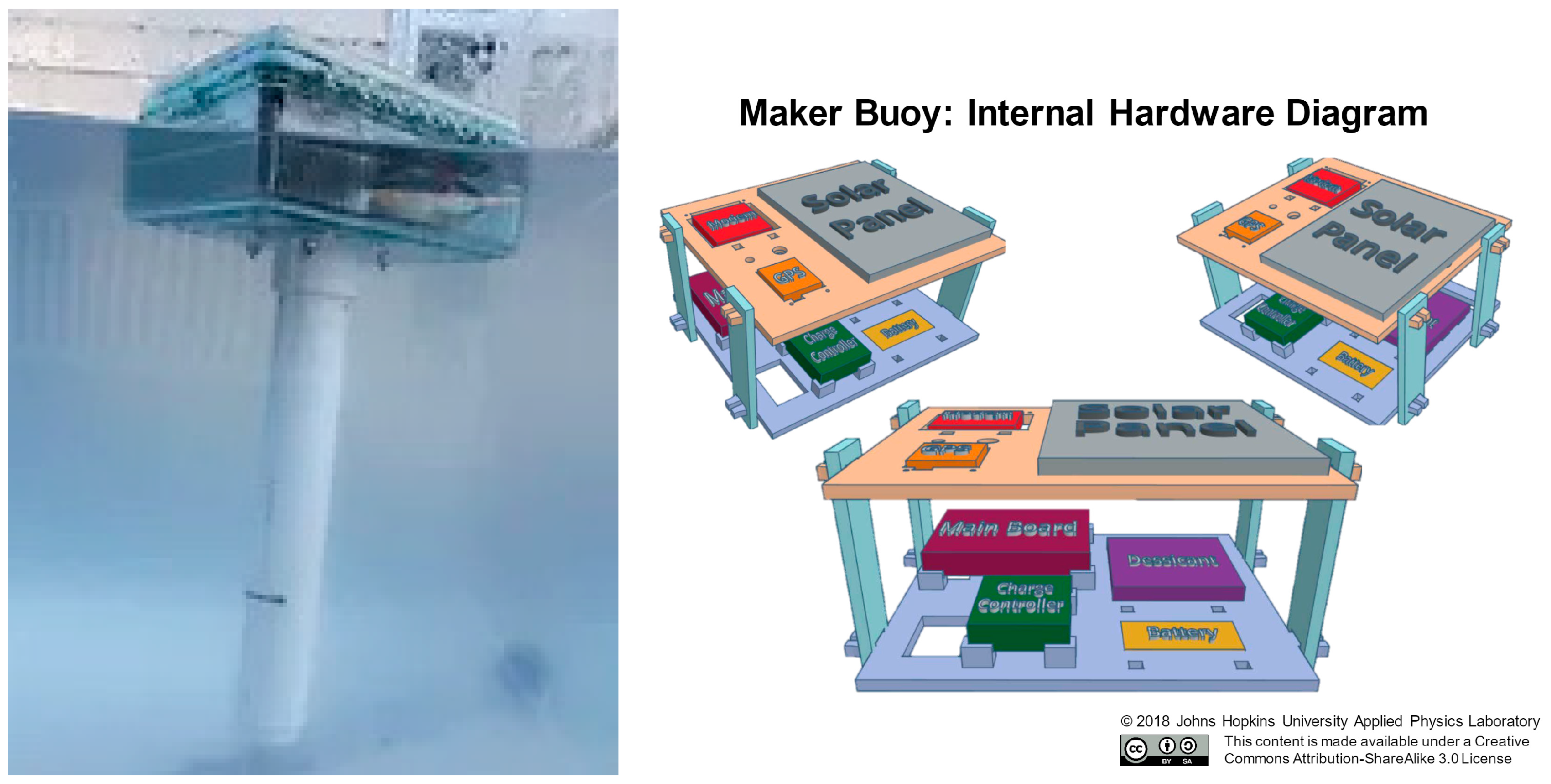
2.1. Characteristics of the Drifters and Trajectory Mapping

The drifters used in this study were low-cost “Maker Buoy” floating drifters based on an open-source hardware platform under a Creative Commons license by Johns Hopkins University Applied Physics Laboratory [30]. These drifters were designed and fabricated by Wayne Pavalko, who is a co-author of this study. A picture of such a drifter is given on the left side of Figure 1. The two drifters (numbered BP002 and BP042) used in this study had the exact same properties and dimensions, which are given in Table 1. The box-shaped topside of the drifter contained the solar panel, GPS sensor, main board, iridium communication units and batteries enclosed in a watertight compartment. To compensate for the topside buoyancy, decrease the windage of the drifter and enable the self-righting mechanism of the buoys, a cylindrical ballast was mounted below the topside case. Other applications of Maker Buoys for research purposes are described in [31]. The ballast weight used for the buoys presented in this study yielded a submergence of 40 cm (5 cm submergence of the topside box).
After being used to evaluate the performance of cleanup systems S001 and S001/B between October 2018 and May 2019 as further detailed in [29], the two drifters were permanently deployed in the GPGP. BP002 was deployed from an MSS-Transporter vessel on 26 June 2019 at coordinates 142.66°W and 33.65°N. BP042 was deployed from an MSS-Transporter vessel on 15 May 2019 at coordinates 145.38°W and 31.38°N. BP002 and BP042 survived 1115 days and 622 days, respectively. The resulting tracks of the drifters are depicted in Figure 2, where the extent of the full trajectories is depicted in the left panel and a close-up view of the convergent event is given in the right panel.

2.2. Post-Processing Steps

In the first part, the convergent event was analyzed. As an initial step, the convergent behavior of the drifters was highlighted by comparing the temporal evolution of the distance between the two drifters with the along-track Eulerian 2D velocity divergence ∇.u at the surface, which was defined as:
. u = u x x + u y y ,
with the surface velocity u ( u x ,   u y ) x and y being, respectively, the zonal and meridional components extracted from an archived analysis of the Hybrid Coordinate Ocean Model (HYCOM) using the Navy Coupled Ocean Data Assimilation (NCODA) system circulation model [32] (Global Ocean Forecast System (GOFS) 3.1 and GLBy0.08 grid experiment [33] with a 0.08° resolution in the longitude, a 0.04° resolution in the latitude, a 6 h timestep and an uppermost cell resolution of 50 cm).
As the next step, the along-track modelled plastic (surface) density (MPSD) ρ p as well as the measured sea-level anomalies (SLAs) were compared during the convergent event period. The MPSD maps were obtained by binning the Lagrangian particles extracted from our operational global plastic dispersal model on a 0.08° × 0.08° resolution grid. This model used the ADVECT dispersal model [34], a 3D dispersal model using the same spatial integration procedure at the surface as [35] and the coastal sources described in the supplementary material of [13]. In short, the dispersal model worked as follows: Lagrangian particles were presumed to be continuously released from coastal-based sources, starting in January 1994 and advected until the present day with a 7 day forecast, thanks to an operational system that was used to steer the ongoing cleanup operations. The forcing used in the operational system was a reanalysis of HYCOM-NCODA data between January 1994 and December 2015 (GOFS 3.1 and GLBy0.08 experiment [36] with a 0.08° resolution in the longitude, a 0.04° resolution in the latitude between 40° S and 40° N and a 0.04° poleward resolution of these latitudes with a 3 h timestep). After December 2015, no HYCOM reanalysis products were available; thus, the dispersal model switched to using the analysis (experiment GOFS 3.1 and GLBy0.08) from January 2016 onwards. Note that this analysis product was the one also used for the divergence analysis detailed in the previous paragraph. To materialize the spatial extent of the tracks in the MPSD map during the convergent event period, the averaged density map during this period is given in Figure 3. The along-track SLA was derived from the Level 4-gridded (0.25° resolution) sea-surface height, measured by the Sentinel-3A and Jason-3A satellites provided by Copernicus Marine Service (CMEMS) [37].
In the second part, the persistency of BP002 in the GPGP was demonstrated by comparing its trajectory with that of the GPGP center. The location of the modelled GPGP center at each time step was obtained by computing the center of gravity of the 5 kg/km2 iso-contour of the 1 month moving average plastic density maps derived from the dispersal model.
Finally, to provide perspective on the significance of the observed behaviors in terms of convergence and persistency, the trajectories of the two drifters were compared with those of historical GDP drifters. The GDP units considered were the undrogued Surface Velocity Program (SVP) drifters [38].

3. Results

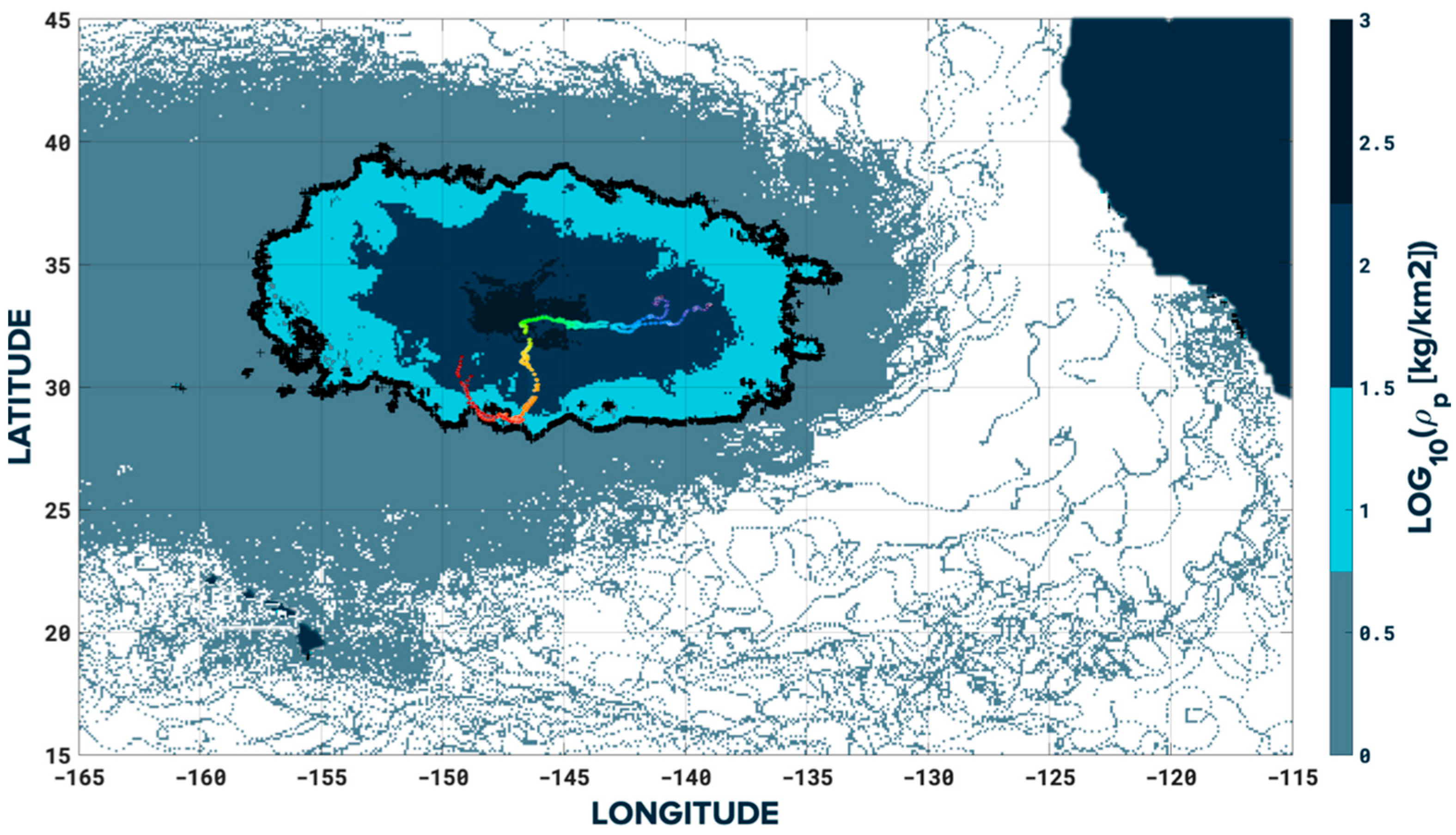
3.1. Convergent Event Analysis

The evolution of the distance between the two drifters was compared with the along-track velocity divergence (one-day rolling average) extracted from the modelled HYCOM-NCODA circulation reanalysis in Figure 4. To highlight the strength of the convergence, a semi-log scale was employed for the distance (navy blue lines). From this figure, a convergent event can be seen between 7 August 2020 and 3 September 2020, where the distance stayed below 10 km for 27 consecutive days. A minimum one-day rolling average distance of 453 m was achieved on 23 August, which also coincided with an area with a persistent negative divergence. Due to an unfortunate loss of satellite communication, no data were available on 21 August and 22 August. Note that the modeled convergence was very local and not necessarily connected to the drifter separation when they were 10–100 km apart. The sensitivity of the outcome to the velocity model was not originally investigated because the aim was to use the legacy model stack in terms of sources and the circulation model, which had been calibrated for its application to the GPGP [13]. Nevertheless, one could argue that the effect of the Stokes drift and wind could have had a significant influence on the outcome, which was not the case during the convergent event, as demonstrated in Appendix A.
Figure 5 shows the evolution of the along-track MPSD as well as the SLA to further highlight the surface convergence. In this figure, it appears that the two drifters had been circulating in areas of high density—above the average density in the GPGP—long before the convergent event (which was already hinted at, looking at Figure 3). The evolution of the encountered MPSD showed strong variations over time (like the oscillations of the divergence). During the convergent event (between the green and red lines), the MPSD reached a local maximum of over 6 times the average density; the SLA experienced a steep increase until reaching a maximum value of 19.5 cm seven days after the end of the convergent event. When comparing the geostrophic circulation quivers derived from the SLA with the trajectories of the drifters, it appeared that the lowest separation of the drifters occurred between two counter-rotating eddies (anti-cyclonic on the west and cyclonic on the east) whilst traveling south towards the outskirts of a stronger mesoscale anti-cyclonic eddy; hence, the increased SLA.
The ability of the dispersal model to capture the convergent event was assessed by first extracting the trajectories of the particles located within a 10 km radius of the mid-point between BP002 and BP042 on 7 August and 3 September, which yielded 93 and 121 tracks, respectively. In Figure 6, the median, top and bottom 5% and 25% quantiles of the daily evolution of the pairwise distance between all those particles (4278 and 7260 pairs) were plotted against 1 / T , where T was the time after (going forward in time) and before (going backward in time) the “release date”. Such a representation is commonly used to infer the diffusion experienced by Lagrangian trackers in different regimes [39]. From this representation, it appeared that the dispersal models performed well in capturing the weak convergence during the first ten days after (resp. before) the start (resp. the end) of the convergent event (top row), whereas the particles diverged before (resp. after) the start (resp. the end) (bottom row). The convergence was, however, not entirely captured, even though the 5% quantile showed a stronger convergence after the first ten days. In the bottom row, the measured data remained between the 25 and 75% quantiles most of the time, which was a good illustration of the ability of the dispersal model to capture the dynamics of the particles around those dates.

3.2. Persistency of BP002 in the GPGP

The 3-year trajectory of BP002 was compared with the trajectory and extent of the GPGP over that period (Figure 7). The GPGP extent corresponded with the limits in longitude and latitude of the 30-day rolling averaged MPSD iso-contour at 1 kg/km2 in a similar fashion as the one depicted in Figure 3 (for 5 kg/km2). The GPGP center coordinates were obtained by weight-averaging the coordinates contained within this iso-contour by the MPSD. In this figure, one can first observe that for both coordinates, they tended to stay within the GPGP boundaries during the 3 years, except for 1 month of the first year (November–December 2019) in latitude, which could be justified by the fact that the initial release location was far from the GPGP center latitude at that time. It also shows that BP002 tended to follow the same oscillations as the GPGP boundaries, but with a much larger amplitude than the GPGP center; this was reasonable, given the way the GPGP center was being tracked. It was also visible that the convergent event occurred when BP002 was very close to the GPGP center. Finally, it appeared that BP002 came very close to where it was released after 3 years of drifting in the GPGP.

3.3. Comparison with SVP Undrogued Drifters

To highlight the fact that observing such behaviors (convergence and persistency) of drifters is very scarce, historical tracks from the GDP program were analyzed. The SVP undrogued drifters were selected because their submergence (17.5 cm) was closest to the Maker Buoy drifters (5 cm for the topside box and 40 cm including the cylindrical ballast); there are also those that are designed to track the uppermost part of the water column. SVP undrogued drifters who had either lost their drogue or were released in the GPGP area (approximated by [160°–120°]W × [20°–40°]N) were considered in the study. Out of approximately 15,000 drifters in the GDP program, 476 drifters matched the criteria mentioned above. First, the cumulative density function (CDF) of the life duration of those drifters (from drogue loss/release to death) was drawn, as shown on the left side of Figure 8. In this figure, it appeared that the operation time of BP002 in the GPGP (1115 days) was higher than 93% of the undrogued drifters; therefore, it stressed the fact that being able to observe the motion of drifters in the GPGP over multiple years is quite rare. In a second step, we only considered the SVP undrogued drifters in the GPGP area, regardless of their drogue loss/release location; in essence, all available SVP undrogued drifters in the GPGP area at a given time. The pairwise distance time series for all the drifter combinations were computed to draw joint histograms between the distance of the pair and the number of days spent at that distance. On the right side of Figure 8, the distance vs. 1 / T P W (invertion of the duration of the pairwise interaction considering T P W ) joint histogram was drawn using the following non-linear intervals: 0, 0.025, 0.05, 0.1, 0.4, 1.6, 6.4, 25.6, 102.4 and 409.6 km for the pairwise distances and 0.125, 0.25, 0.5, 1, 2, 4, 8, 16, 32, 64, 128 and 256 days for the duration T P W within a given distance interval. The distance statistics for the BP002–BP042 combination were compared with this histogram (white crosses in the figure) to highlight the scarcity of observing such a convergent sequence.

4. Discussion

This work relates how, thanks to the analysis of the trajectories of two Maker Buoy drifters deployed in the GPGP between summer 2019 and summer 2022, two specific features of this region of the ocean are evidenced, persistency and convergence, which could lead to hotspot formations.
BP002 and BP042 went through a convergent event for more than a month, which highlighted that a local convergence can be lasting (as shown in Figure 4) and would yield to areas where the local PMD accumulation could be significantly higher than the average (as shown in Figure 5). This heterogeneity within the GPGP is a very important feature because it yielded PMD hotspots with the highest surface densities. When it comes to assessing the feasibility of cleanup operations, the ability to target those hotspots could significantly increase the efficiency of the cleanup and lower the costs. When looking at the evolution of the MPSD values in Figure 5 during the convergent event, it appeared that it was not significantly higher than before the event. This was mainly because this convergence was a local phenomenon, whereas plastic dispersal is non-local and relies on sources, historical accumulation, and complex dynamics. In other words, having a converging current in areas where there is no plastic will not have much impact on the local surface density. Given the extent of the convergent event of the drifters in time and space (more than 4 months below 100 km), it is most likely that the physical processes driving the larger-scale convergence (below 100 km) were mesoscale structures (as both drifters had been experiencing a high SLA and a steep increase during and after the convergent event, as displayed in Figure 5). However, the sub-mesoscale nature of the phenomenon driving the smaller-scale (10 km) convergence cannot be discarded. The comparison between the BP002–BP042 distance and neighboring particles from the plastic dispersal model pairwise distance time evolution (Figure 6) evidenced that the model performed well in capturing the convergence during the first 10 days, but it failed to capture the convergence even for the 5% quantile. Such sub-mesoscale processes [40] as well as a Langmuir circulation [41] could lead to an even smaller-scale heterogeneity. To complement the plastic dispersal model information, we intend to include an assessment of hyperbolic structures such as transient attracting profiles [42].
After the death of BP042, BP002 persisted in the GPGP for more than 3 years, which was a good demonstration that a floating object can remain in the GPGP for several years, as shown in Figure 7. The fact that material that has made its way to the GPGP is unlikely to escape this specific region of the ocean and end up elsewhere or on the shoreline proves that the garbage patches cannot naturally empty themselves over time, even if the inflow of PMD could be stopped. This observation is even more relevant when considering that more than 80% of the GPGP content has been found to be fishing and aquaculture-related equipment, which is specifically built to last in the marine environment [43]. Even though BP002 was shown not to escape the GPGP, a few physical processes were identified as escape routes from the GPGP such as jets and striations; these are evidenced in [44] where, depending on the circulation model considered, it appeared that the higher resolution model yielded more escaping mechanisms. Overall, it has been proven that the mass inside the GPGP has been increasing steadily [13], even though its pace does not quite match the exponential increase in the theoretical inputs into the oceans [45].
We are aware that the conclusions drawn from this small number of drifters have a limited statistical relevance, but they allowed us to make qualitative observations. The scarcity of similar pairwise interactions of SVP undrogued drifters (depicted in the right part of Figure 8) also makes it difficult to assess the abundance of these small-scale features leading to a convergence. Nonetheless, future work could focus on extending the current study to SVP drifters exhibiting a similar time–distance evolution.

Author Contributions

Conceptualization and methodology: B.S.-R.; methodology: B.S.-R.; software: Y.P.; formal analysis: B.S.-R.; writing—review and editing: B.S.-R., Y.P. and W.P. All authors have read and agreed to the published version of the manuscript.

Funding

This research received no external funding.

Institutional Review Board Statement

Not applicable.

Informed Consent Statement

Not applicable.

Data Availability Statement

The data used for this study can be made available upon request to the authors.

Acknowledgments

The authors acknowledge The Ocean Cleanup’s donors and supporters for their ongoing support in funding research and operations. This study was conducted using the GDP program data (https://doi.org/10.25921/7ntx-z961 (accessed on 11 October 2022)) as well at the EU Copernicus Climate Change Service (https://doi.org/10.24381/cds.4c328c78 (accessed on 12 October 2022)). The authors also want to thank the Referees and Academic Editor who contributed to improving the quality of this work.

Conflicts of Interest

The authors declare no conflict of interest.

Appendix A

In this appendix, the influence of the wind on the along-track velocity divergence is assessed. The modelled velocity u was formulated as:
u = u S S C + α . u W ,
where u S S C is the sea-surface current velocity from the HYCOM model described in Section 2.2, u W is the wind velocity at a 10 m altitude obtained from the MERRA2 model [46] and α is a windage coefficient. The results obtained were plotted against the circulation-based divergence for different windages during the convergent period of 1%, 2% and 3% (Figure A1); however, the actual windage of the Maker Buoy would not be more than 1.5%. Values up to 3% were considered to also account for the magnitude of the Stokes drift, which could be approximated by a windage increase of 1.5%, as suggested in [47]. In this figure, it appears that during the convergent event between 1 June 2020 and 1 November 2020, the influence of the windage was very limited.
Figure A1. Scatter plot of circulation divergence vs. modelled velocity divergence for different windage coefficients along the tracks of BP002 and BP042 during the 1 June–1 November 2020 period.
Jmse 11 00068 g0a1

References

  1. UNEP. From Pollution to Solution: A Global Assessment of Marine Litter and Plastic Pollution (Nairobi, 2021); UNEP: Nairobi, Kenya, 2021; ISBN 978-92-807-3881-0. [Google Scholar]
  2. Isobe, A.; Azuma, T.; Cordova, M.R.; Cózar, A.; Galgani, F.; Hagita, R.; Kanhai, L.D.; Imai, K.; Iwasaki, S.; Kako, S.; et al. A multilevel dataset of microplastic abundance in the world’s upper ocean and the Laurentian Great Lakes. Microplastics Nanoplastics 2021, 1, 16. [Google Scholar] [CrossRef]
  3. Meijer, L.J.J.; van Emmerik, T.; van der Ent, R.; Schmidt, C.; Lebreton, L. More than 1000 rivers account for 80% of global riverine plastic emissions into the ocean. Sci. Adv. 2021, 7, 1–14. [Google Scholar] [CrossRef] [PubMed]
  4. van der Mheen, M.; van Sebille, E.; Pattiaratchi, C. Beaching patterns of plastic debris along the Indian Ocean rim. Ocean Sci. Discuss. 2020, 16, 1317–1336. [Google Scholar] [CrossRef]
  5. Eriksen, M.; Lebreton, L.C.M.; Carson, H.S.; Thiel, M.; Moore, C.J.; Borerro, J.C.; Galgani, F.; Ryan, P.G.; Reisser, J. Plastic Pollution in the World’s Oceans: More than 5 Trillion Plastic Pieces Weighing over 250,000 Tons Afloat at Sea. PLoS ONE 2014, 9, e111913. [Google Scholar] [CrossRef] [PubMed] [Green Version]
  6. Available online: https://edition.cnn.com/travel/article/victor-vescovo-deepest-dive-pacific/index.html (accessed on 27 October 2022).
  7. Lacerda, A.L.D.F.; Rodrigues, L.D.S.; Van Sebille, E.; Rodrigues, F.L.; Ribeiro, L.; Secchi, E.R.; Kessler, F.; Proietti, M.C. Plastics in sea surface waters around the Antarctic Peninsula. Sci. Rep. 2019, 9, 3977. [Google Scholar] [CrossRef] [PubMed] [Green Version]
  8. Maximenko, N.; Corradi, P.; Law, K.L.; Van Sebille, E.; Garaba, S.P.; Lampitt, R.S.; Galgani, F.; Martinez-Vicente, V.; Goddijn-Murphy, L.; Veiga, J.M.; et al. Toward the Integrated Marine Debris Observing System. Front. Mar. Sci. 2019, 6, 447. [Google Scholar] [CrossRef] [Green Version]
  9. Jambeck, J.R.; Geyer, R.; Wilcox, C.; Siegler, T.R.; Perryman, M.; Andrady, A.; Narayan, R.; Law, K.L. Plastic waste inputs from land into the ocean. Science 2015, 347, 768–771. [Google Scholar] [CrossRef]
  10. Watson, R.A.; Cheung, W.W.; Anticamara, J.A.; Sumaila, R.U.; Zeller, D.; Pauly, D. Global marine yield halved as fishing intensity redoubles. Fish Fish. 2012, 14, 493–503. [Google Scholar] [CrossRef]
  11. van Sebille, E.; Aliani, S.; Law, K.L.; Maximenko, N.; Alsina, J.M.; Bagaev, A.; Bergmann, M.; Chapron, B.; Chubarenko, I.; Cózar, A.; et al. The physical oceanography of the transport of floating marine debris. Environ. Res. Lett. 2020, 15, 023003. [Google Scholar] [CrossRef] [Green Version]
  12. Available online: www.theoceancleanup.com (accessed on 27 October 2022).
  13. Lebreton, L.; Slat, B.; Ferrari, F.; Sainte-Rose, B.; Aitken, J.; Marthouse, R.; Hajbane, S.; Cunsolo, S.; Schwarz, A.; Levivier, A.; et al. Evidence that the Great Pacific Garbage Patch is rapidly accumulating plastic. Sci. Rep. 2018, 8, 4666. [Google Scholar] [CrossRef]
  14. Egger, M.; Nijhof, R.; Quiros, L.; Leone, G.; Royer, S.J.; McWhirter, A.C.; Kantakov, G.A.; Radchenko, V.I.; Pakhomov, E.A.; Hunt, B.P.; et al. A spatially variable scarcity of floating microplastics in the eastern North Pacific Ocean. Environ. Res. Lett. 2020, 15, 114056. [Google Scholar] [CrossRef]
  15. Reisser, J.; Slat, B.; Noble, K.; du Plessis, K.; Epp, M.; Proietti, M.; de Sonneville, J.; Becker, T.; Pattiaratchi, C. The vertical distribution of buoyant plastics at sea: An observational study in the North Atlantic Gyre. Biogeosciences 2015, 12, 1249–1256. [Google Scholar] [CrossRef] [Green Version]
  16. Egger, M.; Sulu-Gambari, F.; Lebreton, L. First evidence of plastic fallout from the North Pacific Garbage Patch. Sci. Rep. 2020, 10, 7495. [Google Scholar] [CrossRef] [PubMed]
  17. Sainte-Rose, B.; Wrenger, H.; Limburg, H.; Fourny, A.; Tjallema, A. Monitoring and performance evaluation of plastic cleanup systems (part I): Description of the experimental campaign. In Proceedings of the ASME 2020 39th International Conference on Ocean, Offshore and Arctic Engineering, Virtual, 3–7 August 2020; OMAE2020-18885; pp. 1–10. [Google Scholar] [CrossRef]
  18. Niiler, P.P.; Maximenko, N.A.; McWilliams, J.C. Dynamically balanced absolute sea level of the global ocean derived from near-surface velocity observations. Geophys. Res. Lett. 2003, 30, 3–6. [Google Scholar] [CrossRef] [Green Version]
  19. Lumpkin, R.; Centurioni, L.; Perez, R.C. Fulfilling observing system implementation requirements with the global drifter array. J. Atmos. Ocean. Technol. 2016, 33, 685–695. [Google Scholar] [CrossRef]
  20. Elipot, S.; Lumpkin, R.; Perez, R.C.; Lilly, J.M.; Early, J.J.; Sykulski, A.M. A global surface drifter data set at hourly resolution. J. Geophys. Res. Oceans 2016, 121, 2937–2966. [Google Scholar] [CrossRef]
  21. Mignac, D.; Tanajura, C.A.S.; Santana, A.N.; Lima, L.N.; Xie, J. Argo data assimilation into HYCOM with an EnOI method in the Atlantic Ocean. Ocean Sci. 2015, 11, 195–213. [Google Scholar] [CrossRef] [Green Version]
  22. Smit, P.; Houghton, I.; Jordanova, K.; Portwood, T.; Shapiro, E.; Clark, D.; Sosa, M.; Janssen, T. Assimilation of significant wave height from distributed ocean wave sensors. Ocean Model. 2021, 159, 101738. [Google Scholar] [CrossRef]
  23. Laxague, N.J.M.; Özgökmen, T.M.; Haus, B.K.; Novelli, G.; Shcherbina, A.; Sutherland, P.; Guigand, C.M.; Lund, B.; Mehta, S.; Alday, M.; et al. Observations of Near-Surface Current Shear Help Describe Oceanic Oil and Plastic Transport. Geophys. Res. Lett. 2018, 45, 245–249. [Google Scholar] [CrossRef]
  24. van Sebille, E.; Zettler, E.; Wienders, N.; Amaral-Zettler, L.; Elipot, S.; Lumpkin, R. Dispersion of Surface Drifters in the Tropical Atlantic. Front. Mar. Sci. 2021, 7, 607426. [Google Scholar] [CrossRef]
  25. Lumpkin, R.; Özgökmen, T.; Centurioni, L. Advances in the Application of Surface Drifters. Annu. Rev. Mar. Sci. 2017, 9, 59–81. [Google Scholar] [CrossRef] [PubMed] [Green Version]
  26. Van Sebille, E.; England, M.H.; Froyland, G. Origin, dynamics and evolution of ocean garbage patches from observed surface drifters. Environ. Res. Lett. 2012, 7, 044040. [Google Scholar] [CrossRef]
  27. Maximenko, N.; Hafner, J.; Niiler, P. Pathways of marine debris derived from trajectories of Lagrangian drifters. Mar. Pollut. Bull. 2012, 65, 51–62. [Google Scholar] [CrossRef] [PubMed]
  28. Dobler, D.; Maes, C.; Martinez, E.; Rahmania, R.; Gautama, B.G. On the Fate of Floating Marine Debris Carried to the Sea through the Main Rivers of Indonesia. J. Mar. Sci. Eng. 2022, 10, 1009. [Google Scholar] [CrossRef]
  29. Sainte-Rose, B.; Wrenger, H.; Soares, I.; Mosneron-Dupin, C.; Duval, C.; Planchat, A. Monitoring and performance evaluation of plastic cleanup systems (part II): Results and analysis. In Proceedings of the ASME 2020 39th International Conference on Ocean, Offshore and Arctic Engineering, Virtual, 3–7 August 2020; OMAE-18891; pp. 1–7. [Google Scholar] [CrossRef]
  30. Available online:. Available online: https://github.com/wjpavalko/Maker-Buoy (accessed on 10 November 2022).
  31. Carlson, D.F.; Pavalko, W.J.; Petersen, D.; Olsen, M.; Hass, A.E. Maker Buoy variants for water level monitoring and tracking drifting objects in remote areas of Greenland. Sensors 2020, 20, 1254. [Google Scholar] [CrossRef] [Green Version]
  32. Chassignet, E.P.; Hurlburt, H.E.; Metzger, E.J.; Smedstad, O.M.; Cummings, J.A.; Halliwell, G.R.; Bleck, R.; Baraille, R.; Wallcraft, A.J.; Lozano, C.; et al. US GODAE: Global Ocean Prediction with the HYbrid Coordinate Ocean Model (HYCOM). Oceanography 2009, 22, 64–75. [Google Scholar] [CrossRef] [Green Version]
  33. Available online:. Available online: https://www.hycom.org/dataserver/gofs-3pt1/analysis (accessed on 10 August 2022).
  34. Klink, D.; Peytavin, A.; Lebreton, L. Size Dependent Transport of Floating Plastics Modeled in the Global Ocean. Front. Mar. Sci. 2022, 9, 903134. [Google Scholar] [CrossRef]
  35. Lebreton, L.C.M.; Greer, S.D.; Borrero, J.C. Numerical modelling of floating debris in the world’s oceans. Mar. Pollut. Bull. 2012, 64, 653–661. [Google Scholar] [CrossRef]
  36. Available online:. Available online: https://www.hycom.org/dataserver/gofs-3pt1/reanalysis (accessed on 10 August 2022).
  37. Available online:. Available online: https://cds.climate.copernicus.eu/cdsapp#!/dataset/10.24381/cds.4c328c78?tab=overview (accessed on 10 November 2022).
  38. Lumpkin, R.; Pazos, M. Measuring surface currents with Surface Velocity Program drifters: The instrument, its data, and some recent results. In Lagrangian Analysis and Prediction of Coastal and Ocean Dynamics; Cambridge Core: Cambridge, UK, 2009; pp. 39–67. [Google Scholar]
  39. van Sebille, E.; Waterman, S.; Barthel, A.; Lumpkin, R.; Keating, S.R.; Fogwill, C.; Turney, C. Pairwise surface drifter separation in the western Pacific sector of the Southern Ocean. J. Geophys. Res. Oceans 2015, 120, 6769–6781. [Google Scholar] [CrossRef] [Green Version]
  40. McWilliams, J.C. Submesoscale currents in the ocean. Proc. R. Soc. A Math. Phys. Eng. Sci. 2016, 472, 20160117. [Google Scholar] [CrossRef] [Green Version]
  41. Thorpe, S.A. Langmuir circulation. Annu. Rev. Fluid Mech. 2004, 36, 55–79. [Google Scholar] [CrossRef]
  42. Serra, M.; Sathe, P.; Rypina, I.; Kirincich, A.; Ross, S.D.; Lermusiaux, P.; Allen, A.; Peacock, T.; Haller, G. Search and rescue at sea aided by hidden flow structures. Nat. Commun. 2020, 11, 2525. [Google Scholar] [CrossRef] [PubMed]
  43. Lebreton, L.; Royer, S.-J.; Peytavin, A.; Strietman, W.J.; Smeding-Zuurendonk, I.; Egger, M. Industrialised fishing nations largely contribute to floating plastic pollution in the North Pacific subtropical gyre. Sci. Rep. 2022, 12, 12666. [Google Scholar] [CrossRef] [PubMed]
  44. Maes, C.; Blanke, B.; Martinez, E. Origin and fate of surface drift in the oceanic convergence zones of the eastern Pacific. Geophys. Res. Lett. 2016, 43, 3398–3405. [Google Scholar] [CrossRef] [Green Version]
  45. Lebreton, L.; Andrady, A. Future scenarios of global plastic waste generation and disposal. Palgrave Commun. 2019, 5, 6. [Google Scholar] [CrossRef] [Green Version]
  46. Global Modeling and Assimilation Office (GMAO). inst3_3d_asm_Cp: MERRA-2 3D IAU State, Meteorology Instantaneous 3-Hourly (p-coord, 0.625x0.5L42), Version 5.12.4; Goddard Space Flight Center Distributed Active Archive Center (GSFC DAAC): Greenbelt, MD, USA, 2015. [Google Scholar] [CrossRef]
  47. Tamura, H.; Miyazawa, Y.; Oey, L.-Y. The Stokes drift and wave induced-mass flux in the North Pacific. J. Geophys. Res. Earth Surf. 2012, 117, C08021. [Google Scholar] [CrossRef]
Figure 1. (Left) panel: picture of a Maker Buoy drifter sitting inside water. (Right) panel: a 3D visualization of the electronics layout inside the topside compartment.
Jmse 11 00068 g001
Figure 2. Left panel: BP042 and BP002 drifter trajectories (between 28 June 2019 and 28 June 2022) framed around the North-East Pacific between Hawaii and California; green and red symbols correspond with the start and end locations of the tracks, respectively. Right panel: zoom on the convergent event period between 1 June 2020 and 1 November 2020.
Jmse 11 00068 g002
Figure 3. Background color: 30 day averaged modelled plastic surface density (MPSD) map in August 2020 ( ρ p expressed in kg/km2) in logarithmic scale; thick black line (between grey–blue and light blue colors): iso-contour of ρ p = 5 kg/km2; rainbow-colored dots: tracks of the drifters during the convergent event period between 1 June 2020 and 1 November 2020.
Jmse 11 00068 g003
Figure 4. Light blue: velocity divergence for the two drifters BP002 (solid line) and BP042 (dotted line), 24 h averages; navy blue: distance between the two drifters, 24 h averages (logarithmic scale used to account for the theoretical exponential evolution of distance in a uniform divergence); grey–blue solid line: 0 divergence. The start and end of the convergent episode are evidenced by the green and red lines, respectively (7 August to 3 September).
Jmse 11 00068 g004
Figure 5. Light blue: encountered MPSD for the two drifters BP002 (solid line) and BP042 (dotted line), 24 h averages; navy blue: evolution of the sea-level anomaly (SLA) for the two drifters BP002 (solid line) and BP042 (dotted line); solid grey–blue line: averaged plastic density in the GPGP (materialized by the area inside the thick black line contour of Figure 3). The start and end of the convergent episode are evidenced by the green and red lines, respectively (7 August to 3 September).
Jmse 11 00068 g005
Figure 6. 1 / T as a function of the measured distance between BP002 and BP042 and the pairwise distances of Lagrangian particles located within a 10 km radius of the middle point between the two drifters. The median (light blue dots), 5% and 95% (light grey dots), 25% and 75% (navy blue dots) quantiles of the pairwise distances were compared with the measured 1 day averaged distance between BP002 and BP042 (grey–blue line). Four configurations were studied at the end and start of the convergent event (top left and right): after 7 August and before 3 September (bottom left and right), before 7 August and after 3 September. The start and end of the convergent episode are evidenced by the green and red lines, respectively.
Jmse 11 00068 g006
Figure 7. Evolution of the longitude (top) and latitude (bottom) of BP002 (light blue solid line) and the center of the GPGP (dark blue dotted line) with the extent of the GPGP highlighted by the gray area. The start and end of the convergent event are materialized by the red and green lines, respectively.
Jmse 11 00068 g007
Figure 8. Left: CDF of operation duration of undrogued GDP drifters (in dark blue) and operation duration of BP002 (1115 days) in dotted light blue. Right: joint histograms between pairwise distance and duration inverse 1 / T P W . The statistics for the BP002–BP042 distances are materialized by the white cross.
Jmse 11 00068 g008
Table 1. Geometrical characteristics of the Maker Buoy drifters.
DimensionValue (cm)
Topside height10
Topside length20
Topside width17
Ballast tube height35
Ballast tube diameter3
Disclaimer/Publisher’s Note: The statements, opinions and data contained in all publications are solely those of the individual author(s) and contributor(s) and not of MDPI and/or the editor(s). MDPI and/or the editor(s) disclaim responsibility for any injury to people or property resulting from any ideas, methods, instructions or products referred to in the content.

