
Long-Strip Target Detection and Tracking with Autonomous Surface Vehicle


Abstract
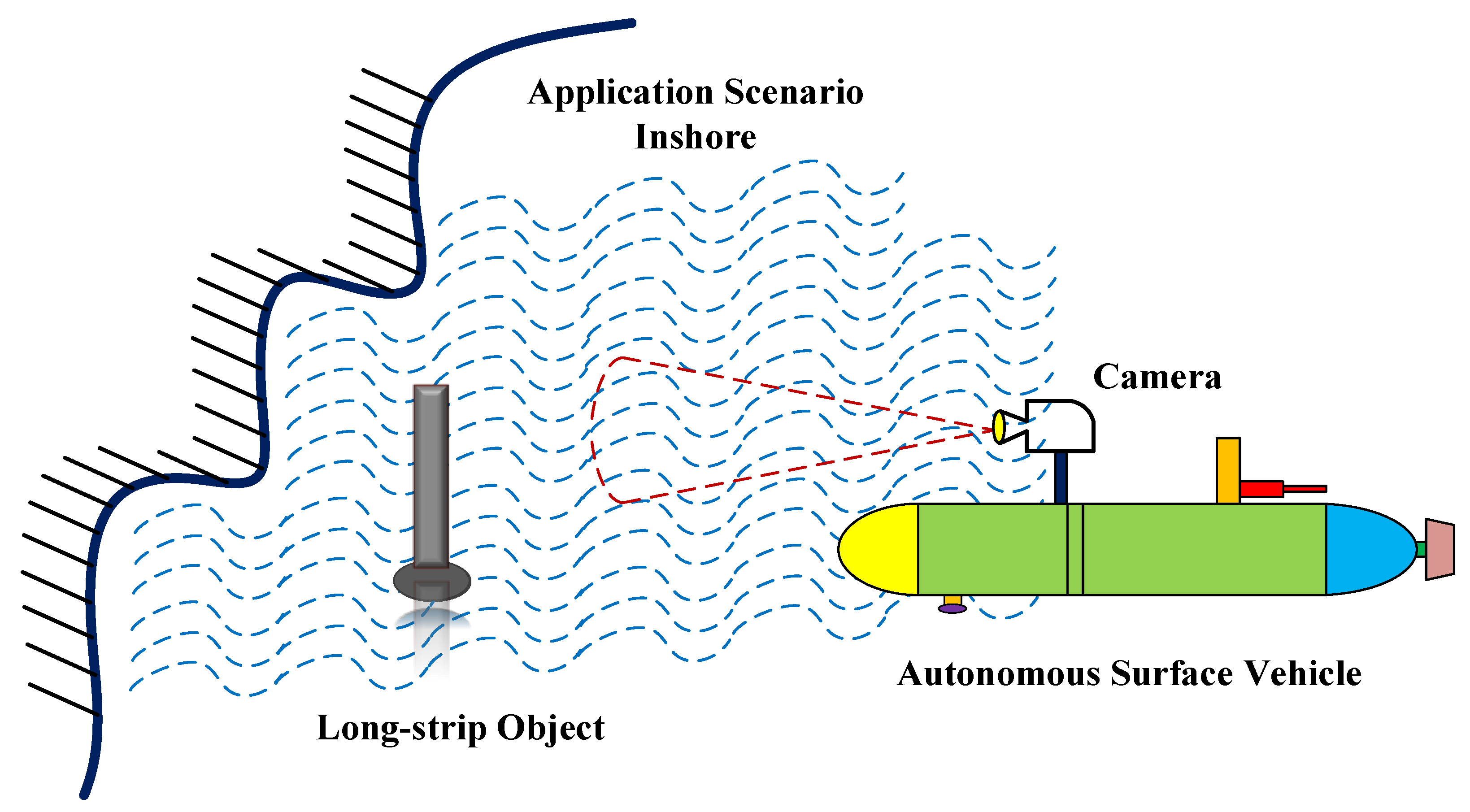
1. Introduction
2. System Framework and Problem Statement
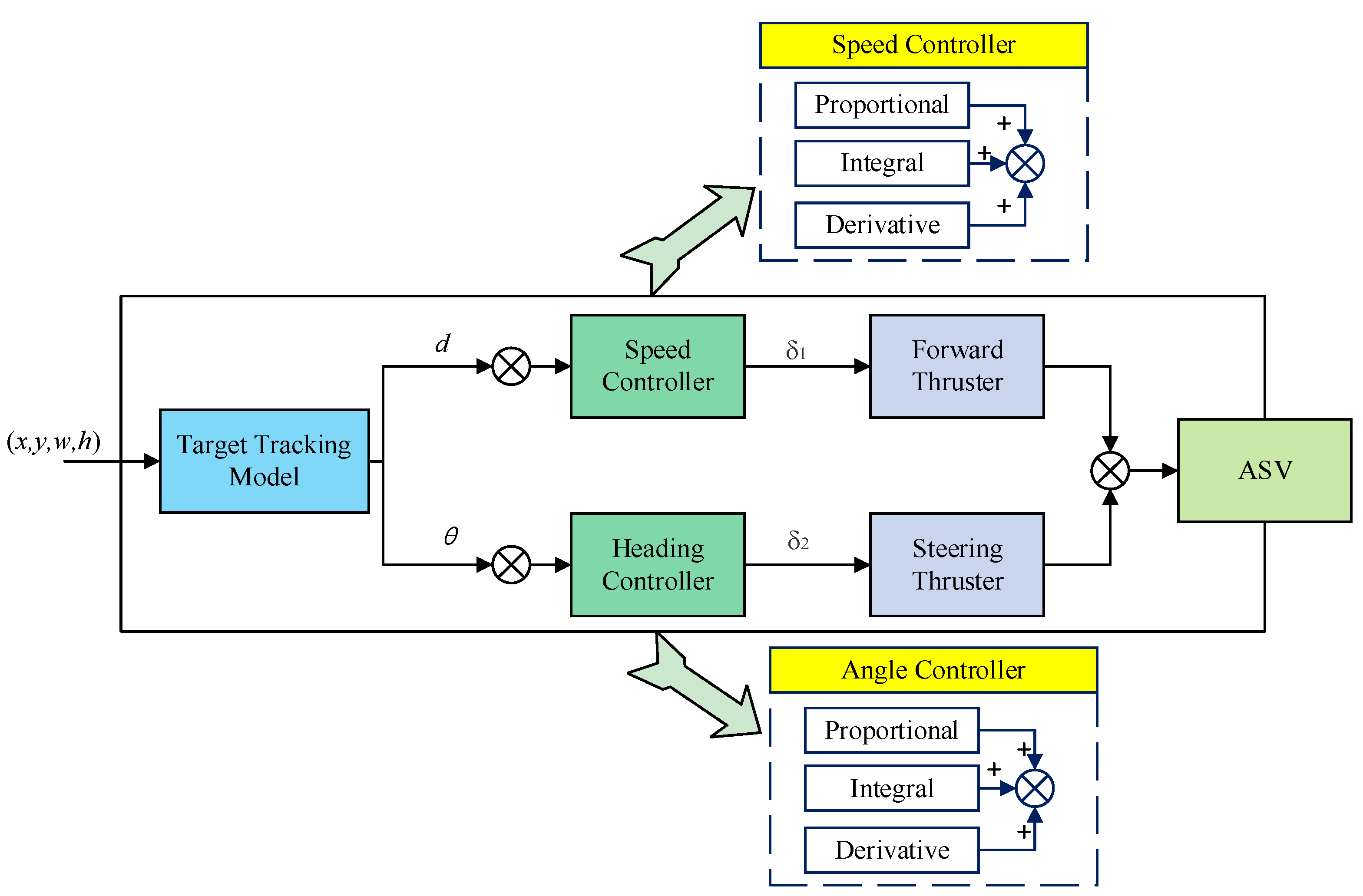
2.1. System Framework
2.2. Dynamic Model of ASV
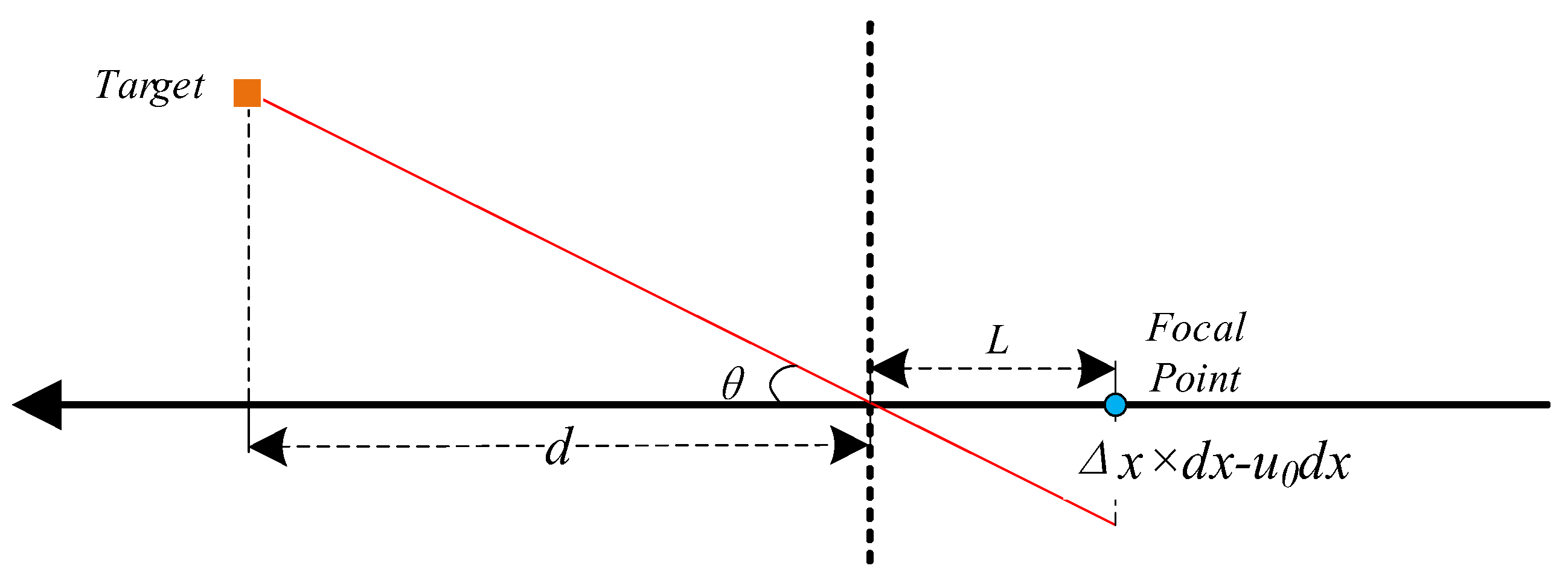
2.3. Problem Description
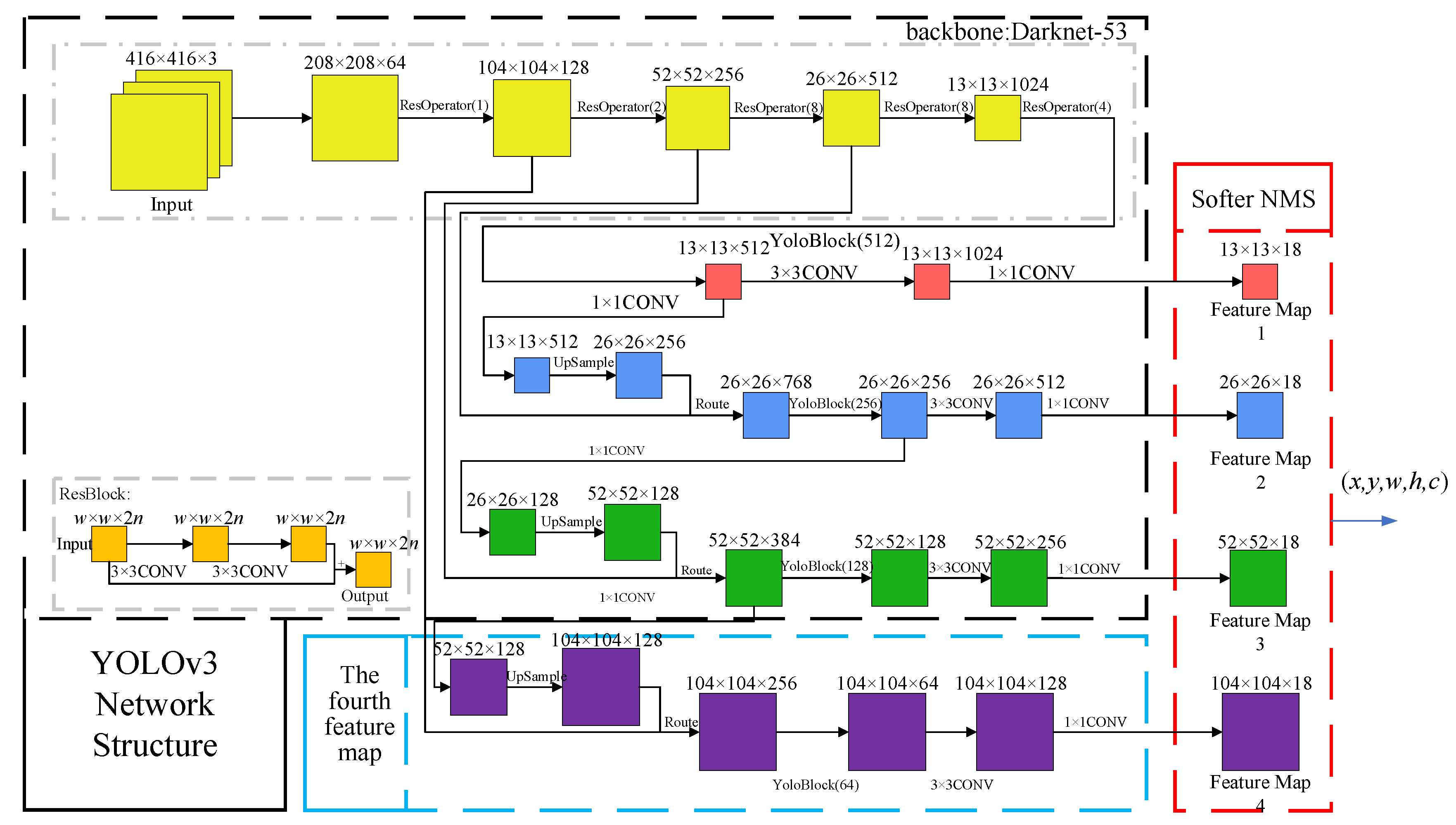
3. YOLO–Softer-NMS-Based Target Detection Algorithm
3.1. Improved Network Structure for YOLO–Softer NMS
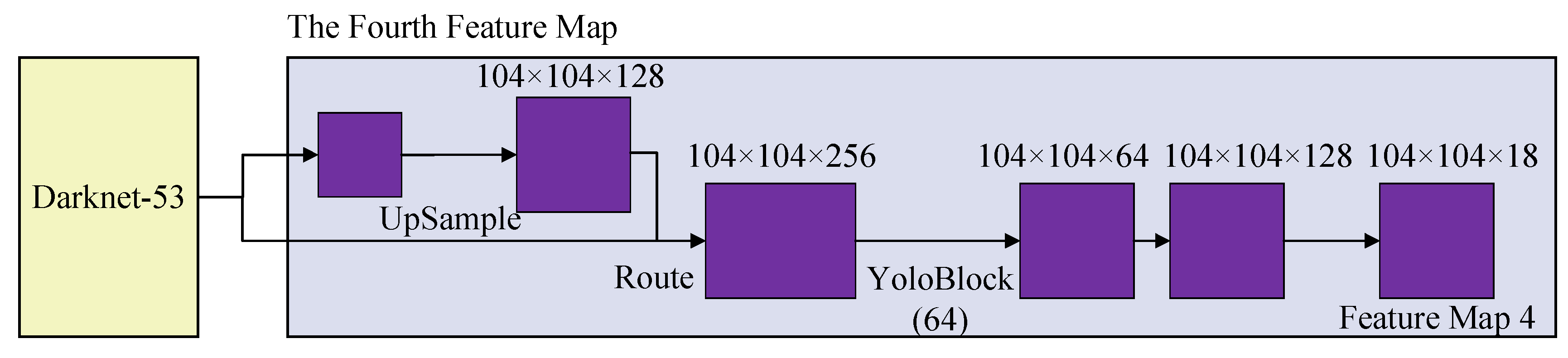
3.2. The Fourth Feature Map Improvement
3.3. Softer NMS Improvement
4. Target Tracking Model of Autonomous Surface Vehicle
4.1. Target DetectionMethod
4.2. Target Tracking Method
5. Experiments and Results
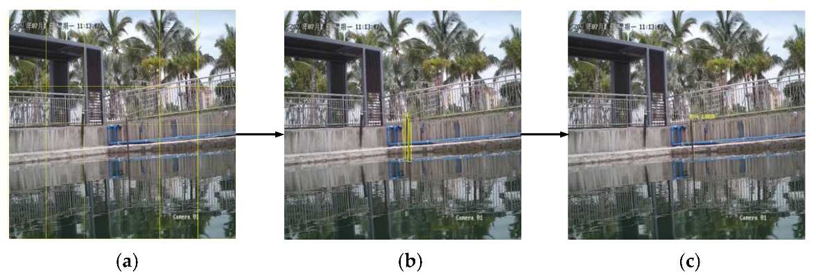
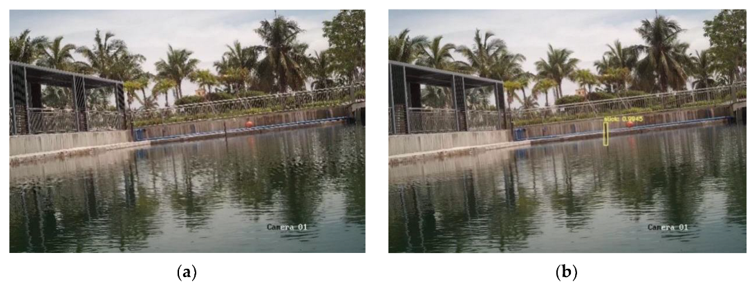
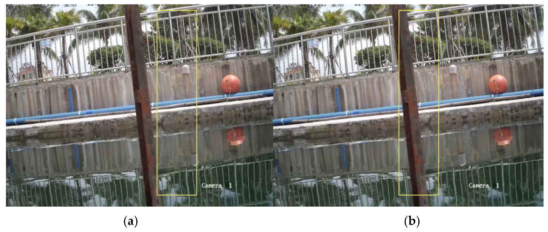
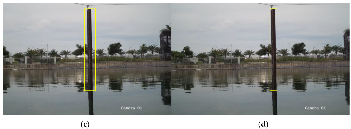
5.1. Target Detection Results
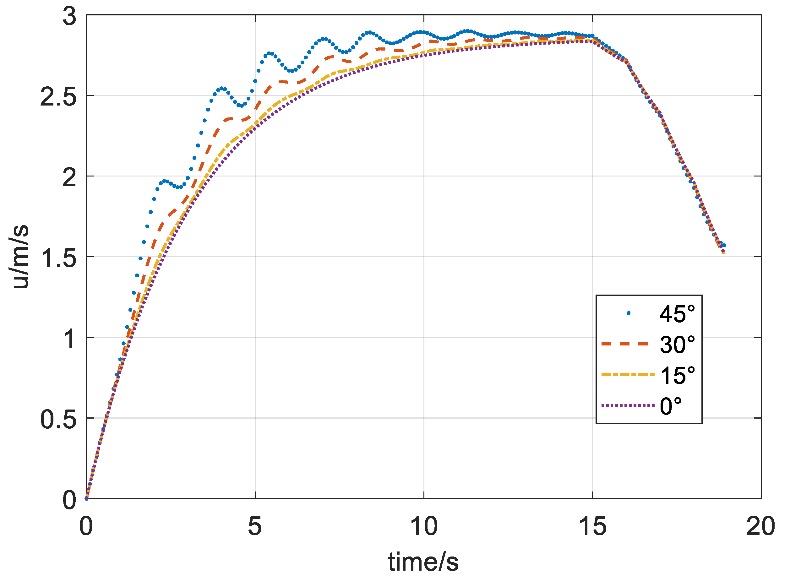
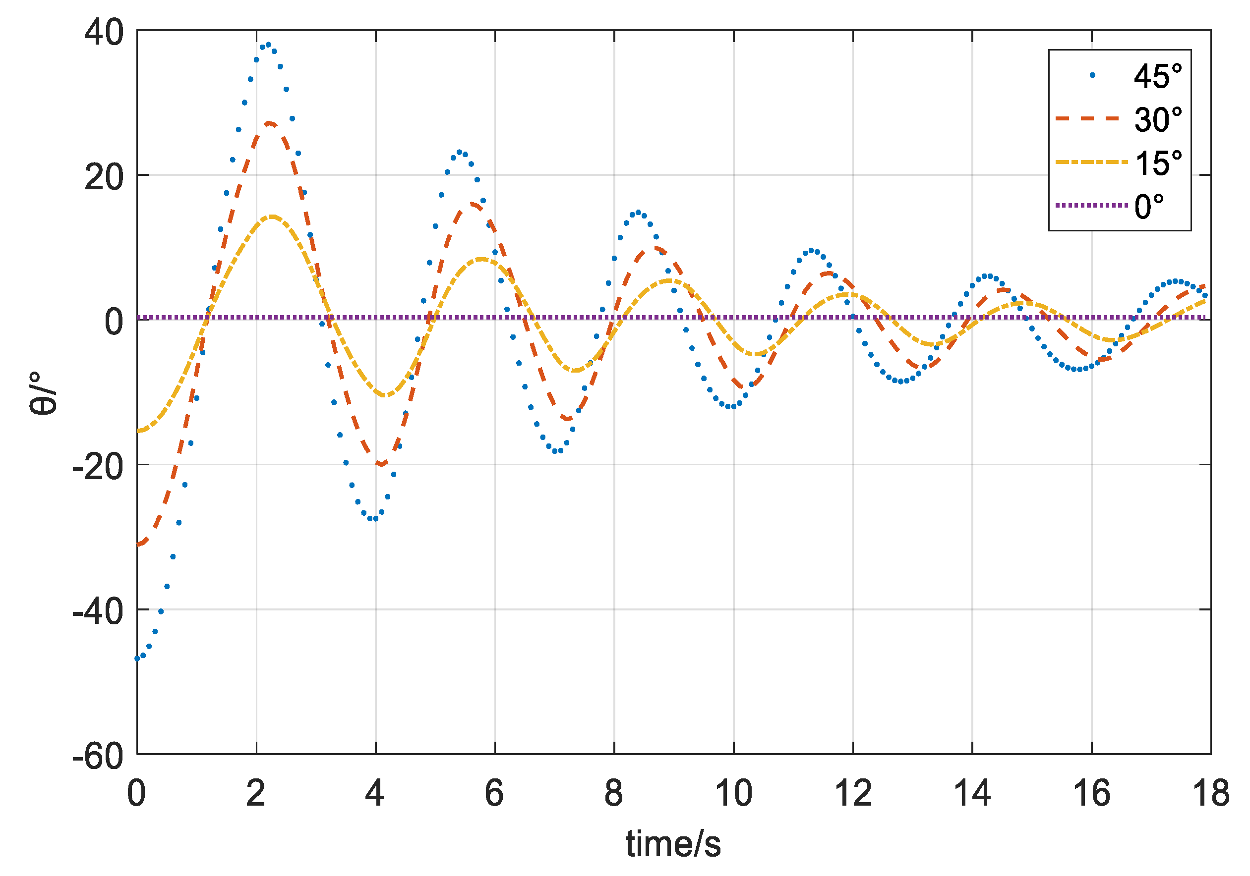
5.2. Motion Control Results
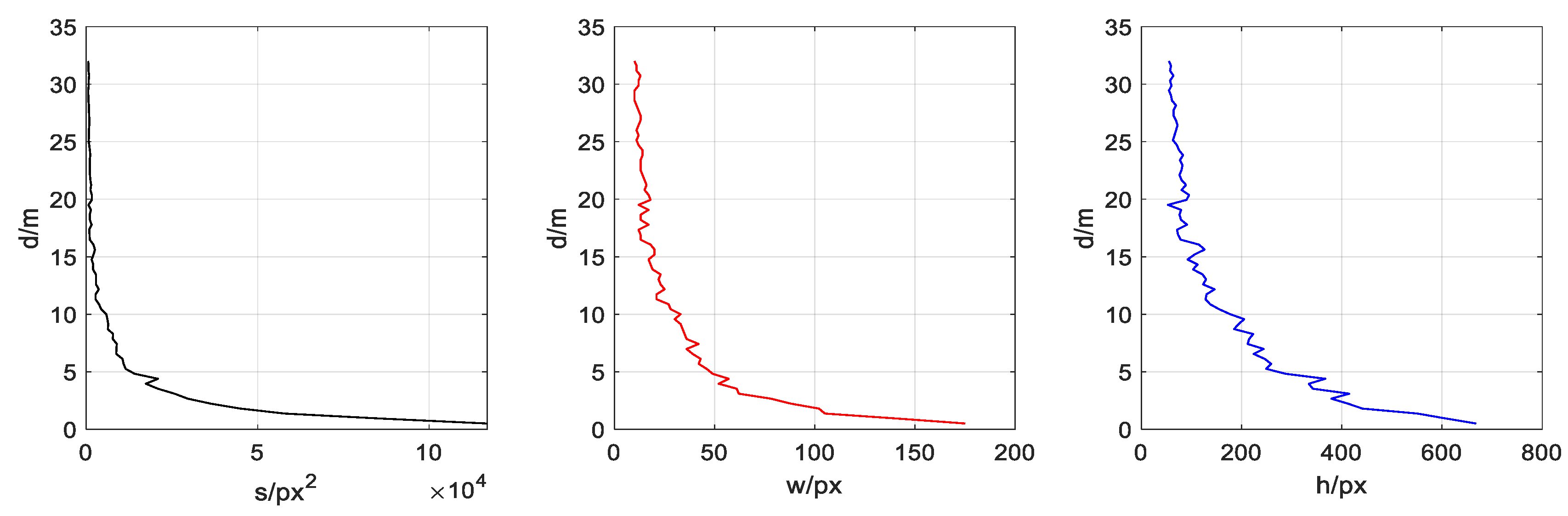
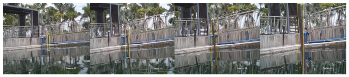
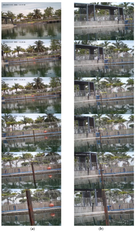
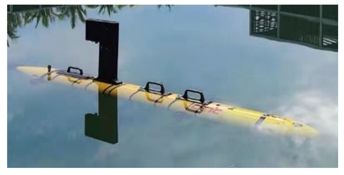
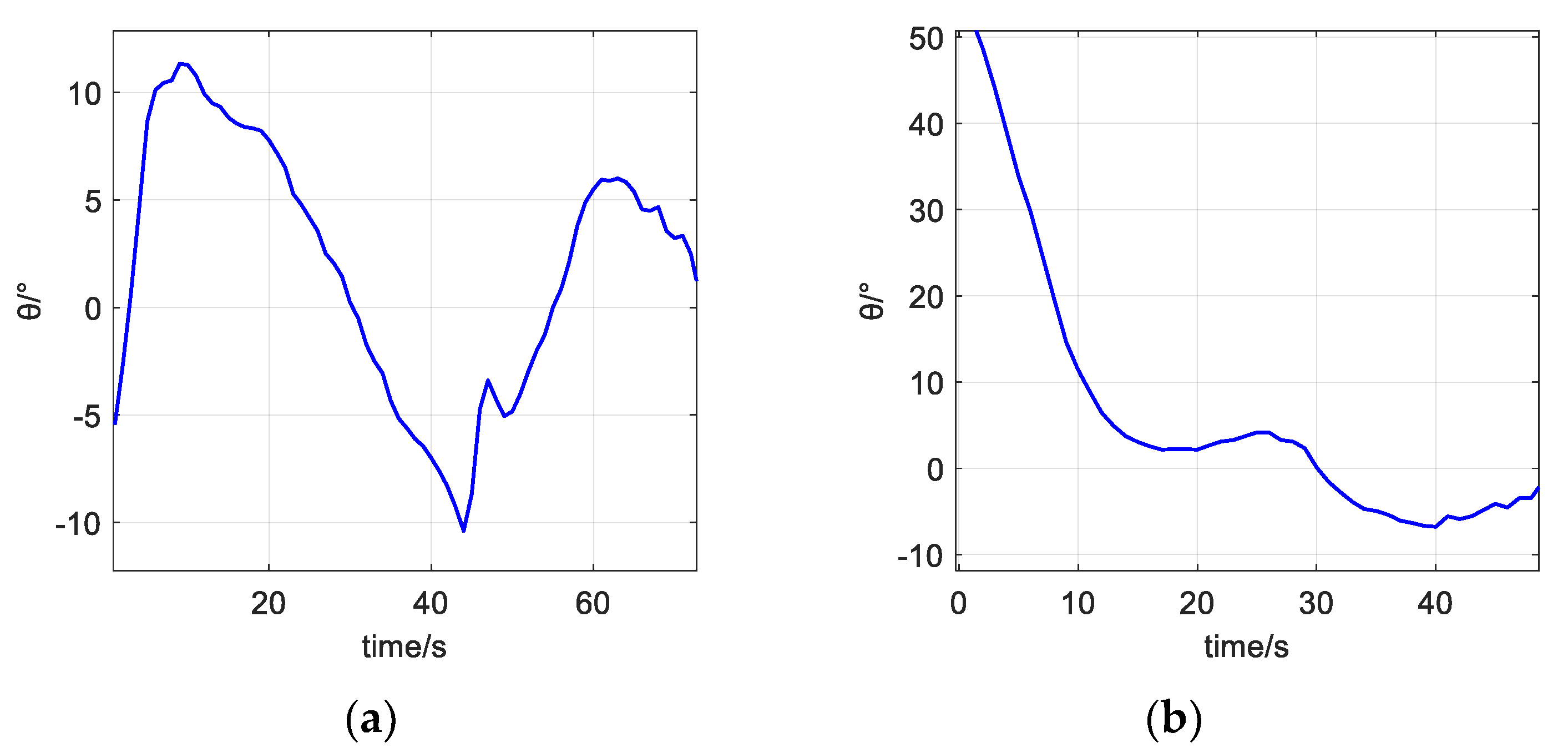
5.3. Lake Test Results
6. Conclusions
Author Contributions
Funding
Institutional Review Board Statement
Informed Consent Statement
Data Availability Statement
Conflicts of Interest
References
- Teixeira, E.; Araujo, B.; Costa, V.; Mafra, S.; Figueiredo, F. Literature Review on Ship Localization, Classification, and Detection Methods Based on Optical Sensors and Neural Networks. Sensors 2022, 22, 6879. [Google Scholar] [CrossRef] [PubMed]
- Liang, J.-M.; Mishra, S.; Cheng, Y.-L. Applying Image Recognition and Tracking Methods for Fish Physiology Detection Based on a Visual Sensor. Sensors 2022, 22, 5545. [Google Scholar] [CrossRef] [PubMed]
- Vagale, A.; Oucheikh, R.; Bye, R.T.; Osen, O.L.; Fossen, T.I. Path planning and collision avoidance for autonomous surface vehicles I: A review. J. Mar. Sci. Technol. 2021, 26, 1292–1306. [Google Scholar] [CrossRef]
- Zhang, X.D.; Liu, S.L.; Liu, Y.; Hu, X.F.; Gao, C. Review on development trend of launch and recovery technology for USV. Chin. J. Ship Res. 2018, 13, 50–57. [Google Scholar]
- Liu, W.; Liu, Y.; Bucknall, R. A Robust Localization Method for Unmanned Surface Vehicle (USV) Navigation Using Fuzzy Adaptive Kalman Filtering. IEEE Access 2019, 7, 46071–46083. [Google Scholar] [CrossRef]
- Busquets, J.; Zilic, F.; Aron, C.; Manzoliz, R. AUV and ASV in twinned navigation for long term multipurpose survey applications. In Proceedings of the MTS/IEEE OCEANS, Bergen, Norway, 10–14 June 2013. [Google Scholar]
- Wu, J.; Liu, J.; Xu, H. A variable buoyancy system and a recovery system developed for a deep-sea AUV Qianlong I. In Proceedings of the OCEANS 2014, Taipei, Taiwan, 7–10 April 2014. [Google Scholar]
- Venkatesan, S. AUV for Search & Rescue at sea—An innovative approach. In Proceedings of the 2016 IEEE/OES Autonomous Underwater Vehicles (AUV), Tokyo, Japan, 6–9 November 2016; pp. 1–9. [Google Scholar]
- Martins, R.; De Sousa, J.B.; Afonso, C.C.; Incze, M.L. REP10 AUV: Shallow water operations with heterogeneous autonomous vehicles. In Proceedings of the OCEANS 2011 IEEE—Spain, Santander, Spain, 6–9 June 2011. [Google Scholar]
- Rashid, M.; Roy, R.; Ahsan, M.M.; Siddique Design, Z. Design and Development of an Autonomous Surface Vehicle for Water Quality Monitoring. Electr. Eng. Syst. Sci. 2022, 1, 1–14. [Google Scholar] [CrossRef]
- Im, S.; Kim, D.; Cheon, H.; Ryu, J. Object Detection and Tracking System with Improved DBSCAN Clustering Using Radar on Unmanned Surface Vehicle. In Proceedings of the 2021 21st International Conference on Control, Automation and Systems (ICCAS), Jeju, Korea, 12–15 October 2021. [Google Scholar]
- Xu, H.X.; Jiang, C.L. Heterogeneous oceanographic exploration system based on USV and AUV: A survey of developments and challenges. J. Univ. Chin. Acad. Sci. 2021, 38, 145–159. [Google Scholar]
- Yang, Z.; Li, Y.; Wang, B.; Ding, S.; Jiang, P. A Lightweight Sea Surface Object Detection Network for Unmanned Surface Vehicles. J. Mar. Sci. Eng. 2022, 10, 965. [Google Scholar] [CrossRef]
- Park, H.; Ham, S.-H.; Kim, T.; An, D. Object Recognition and Tracking in Moving Videos for Maritime Autonomous Surface Ships. J. Mar. Sci. Eng. 2022, 10, 841. [Google Scholar] [CrossRef]
- Masita, K.L.; Hasan, A.N.; Shongwe, T. Deep Learning in Object Detection: A Review. In Proceedings of the International Conference on Artificial Intelligence, Big Data, Computing and Data Communication Systems (icABCD), Durban, South Africa, 6–7 August 2020; pp. 1–11. [Google Scholar]
- Li, X.; Nishida, Y.; Myint, M.; Yonemori, K.; Mukada, N.; Lwin, K.N.; Takayuki, M.; Minami, M. Dual-eyes vision-based docking experiment of AUV for sea bottom battery recharging. In Proceedings of the OCEANS 2017—Aberdeen, Aberdeen, UK, 19–22 June 2017; pp. 1–5. [Google Scholar]
- Neves, G.; Cerqueira, R.; Albiez, J.; Oliveira, L. Rotation-invariant shipwreck recognition with forward-looking sonar. Comput. Vis. Pattern Recognit. 2019, 1, 1–14. [Google Scholar] [CrossRef]
- Maire, F.; Prasser, D.; Dunbabin, M.D.; Ict, C.; Dawson, M. A Vision Based Target Detection System for Docking of an Autonomous Underwater Vehicle. In Proceedings of the Australasian Conference on Robotics and Automation (ACRA), Sydney, Australia, 2–4 December 2009; pp. 1–7. [Google Scholar]
- Zhang, Y.H.; Wu, S.; Liu, Z.H.; Yang, Y.J.; Zhu, D.; Chen, Q. A real-time detection USV algorithm based on bounding box regression. J. Phys. Conf. Ser. 2020, 1544, 12–22. [Google Scholar] [CrossRef]
- Jin, J.; Zhang, J.; Liu, D.; Shi, J.; Wang, D.; Li, F. Vision-Based Target Tracking for Unmanned Surface Vehicle Considering Its Motion Features. IEEE Access 2020, 8, 132655–132664. [Google Scholar] [CrossRef]
- Liu, H.; Sun, F.; Gu, J.; Deng, L. SF-YOLOv5: A Lightweight Small Object Detection Algorithm Based on Improved Feature Fusion Mode. Sensors 2022, 22, 5817. [Google Scholar] [CrossRef] [PubMed]
- Ren, S.; He, K.; Girshick, R.; Sun, J. Faster R-CNN: Towards Real-Time Object Detection with Region Proposal Networks. IEEE Trans. Pattern Anal. Mach. Intell. 2017, 39, 1137–1149. [Google Scholar] [CrossRef] [PubMed]
- Redmon, J.; Divvala, S.; Girshick, R.; Farhadi, A. You Only Look Once: Unified, Real-Time Object Detection. In Proceedings of the 2016 IEEE Conference on Computer Vision and Pattern Recognition (CVPR), Las Vegas, NV, USA, 27–30 June 2016; pp. 779–788. [Google Scholar]
- Liu, W.; Anguelov, D.; Erhan, D.; Szegedy, C.; Reed, S.; Fu, C.-Y.; Berg, A.C. SSD: Single Shot MultiBox Detector. In Lecture Notes in Computer Science; Lecture Notes in Computer Science: Berlin/Heidelberg, Germany, 2016; pp. 21–37. [Google Scholar]
- Kulkarni, M.; Junare, P.; Deshmukh, M.; Rege, P.P. Visual SLAM Combined with Object Detection for Autonomous Indoor Navigation Using Kinect V2 and ROS. In Proceedings of the 2021 IEEE 6th International Conference on Computing, Communication and Automation (ICCCA), New Delhi, India, 17–19 December 2021; pp. 478–482. [Google Scholar]
- Chen, B.; Peng, G.; He, D.; Zhou, C.; Hu, B. Visual SLAM Based on Dynamic Object Detection. In Proceedings of the 2021 33rd Chinese Control and Decision Conference (CCDC), Kunming, China, 22–24 May 2021; pp. 5966–5971. [Google Scholar]
- Hu, J.; Fang, H.; Yang, Q.; Zha, W. MOD-SLAM: Visual SLAM with Moving Object Detection in Dynamic Environments. In Proceedings of the 40th Chinese Control Conference (CCC), Shanghai, China, 26–28 July 2021; pp. 4302–4307. [Google Scholar]
- Li, Y.; Zhang, X.; Shen, Z. YOLO-Submarine Cable: An Improved YOLO-V3 Network for Object Detection on Submarine Cable Images. J. Mar. Sci. Eng. 2022, 10, 1143. [Google Scholar] [CrossRef]
- Kim, J.-H.; Kim, N.; Park, Y.W.; Won, C.S. Object Detection and Classification Based on YOLO-V5 with Improved Maritime Dataset. J. Mar. Sci. Eng. 2022, 10, 377. [Google Scholar] [CrossRef]
- Liu, T.; Pang, B.; Zhang, L.; Yang, W.; Sun, X. Sea Surface Object Detection Algorithm Based on YOLO v4 Fused with Reverse Depthwise Separable Convolution (RDSC) for USV. J. Mar. Sci. Eng. 2021, 9, 753. [Google Scholar] [CrossRef]
- Yildiz, Ö.; Gökalp, R.B.; Yilmaz, A.E. A review on motion control of the Underwater Vehicles. In Proceedings of the 2009 International Conference on Electrical and Electronics Engineering—ELECO 2009, Bursa, Turkey, 5–8 November 2009; pp. II-337–II-341. [Google Scholar]
- He, Y.H.; Zhu, C.C.; Wang, J.R.; Savvides, M.; Zhang, X.Y. Bounding Box Regression with Uncertainty for Accurate Object Detection. In Proceedings of the IEEE Conference on Computer Vision and Pattern Recognition (CVPR), Long Beach, CA, USA, 15–20 June 2019. [Google Scholar]


| Notation | Meanings |
|---|---|
| M | Inertia matrix |
| Coriolis and centrifugal terms matrix | |
| D | Damping matrix |
| τ | Force and moment of ASV |
| v = [u, v, r]T | Velocity vector |
| η = [x, y, ψ]T | Position vector |
| J(η) | Conversion matrix |
| IOU | Standard indicator |
| s = w × h | Width and length |
| Angle deviation | |
| d | Distance between ASV and target |
| Model | mAP (%) | Speed (FPS) |
|---|---|---|
| Faster-RCNN | 85.67% | 16 |
| YOLOv3 | 92.52% | 27 |
| YOLO–Softer NMS | 97.09% | 27 |
Disclaimer/Publisher’s Note: The statements, opinions and data contained in all publications are solely those of the individual author(s) and contributor(s) and not of MDPI and/or the editor(s). MDPI and/or the editor(s) disclaim responsibility for any injury to people or property resulting from any ideas, methods, instructions or products referred to in the content. |
© 2023 by the authors. Licensee MDPI, Basel, Switzerland. This article is an open access article distributed under the terms and conditions of the Creative Commons Attribution (CC BY) license (https://creativecommons.org/licenses/by/4.0/).
Share and Cite
Zhang, M.; Zhao, D.; Sheng, C.; Liu, Z.; Cai, W. Long-Strip Target Detection and Tracking with Autonomous Surface Vehicle. J. Mar. Sci. Eng. 2023, 11, 106. https://doi.org/10.3390/jmse11010106
Zhang M, Zhao D, Sheng C, Liu Z, Cai W. Long-Strip Target Detection and Tracking with Autonomous Surface Vehicle. Journal of Marine Science and Engineering. 2023; 11(1):106. https://doi.org/10.3390/jmse11010106
Chicago/Turabian StyleZhang, Meiyan, Dongyang Zhao, Cailiang Sheng, Ziqiang Liu, and Wenyu Cai. 2023. "Long-Strip Target Detection and Tracking with Autonomous Surface Vehicle" Journal of Marine Science and Engineering 11, no. 1: 106. https://doi.org/10.3390/jmse11010106
APA StyleZhang, M., Zhao, D., Sheng, C., Liu, Z., & Cai, W. (2023). Long-Strip Target Detection and Tracking with Autonomous Surface Vehicle. Journal of Marine Science and Engineering, 11(1), 106. https://doi.org/10.3390/jmse11010106