
A Multi-Strategy Framework for Coastal Waste Detection


Abstract
:1. Introduction
2. Related Works
3. Background
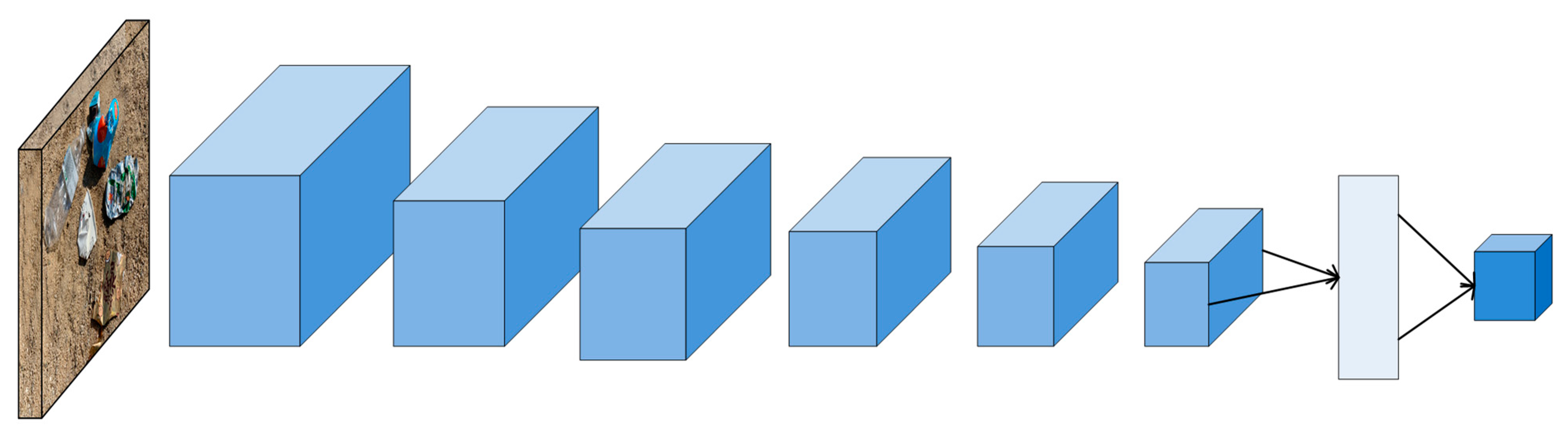
3.1. YOLO
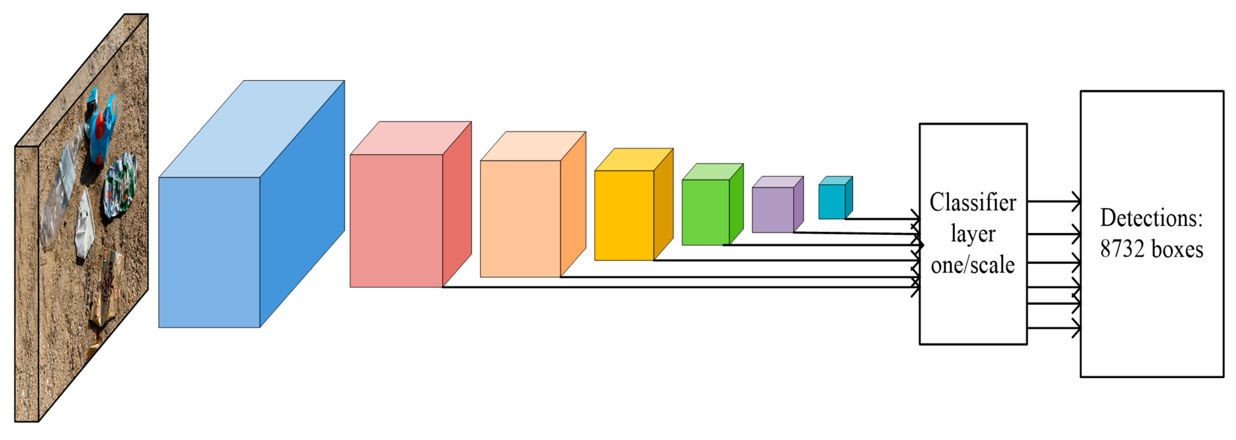
3.2. SSD
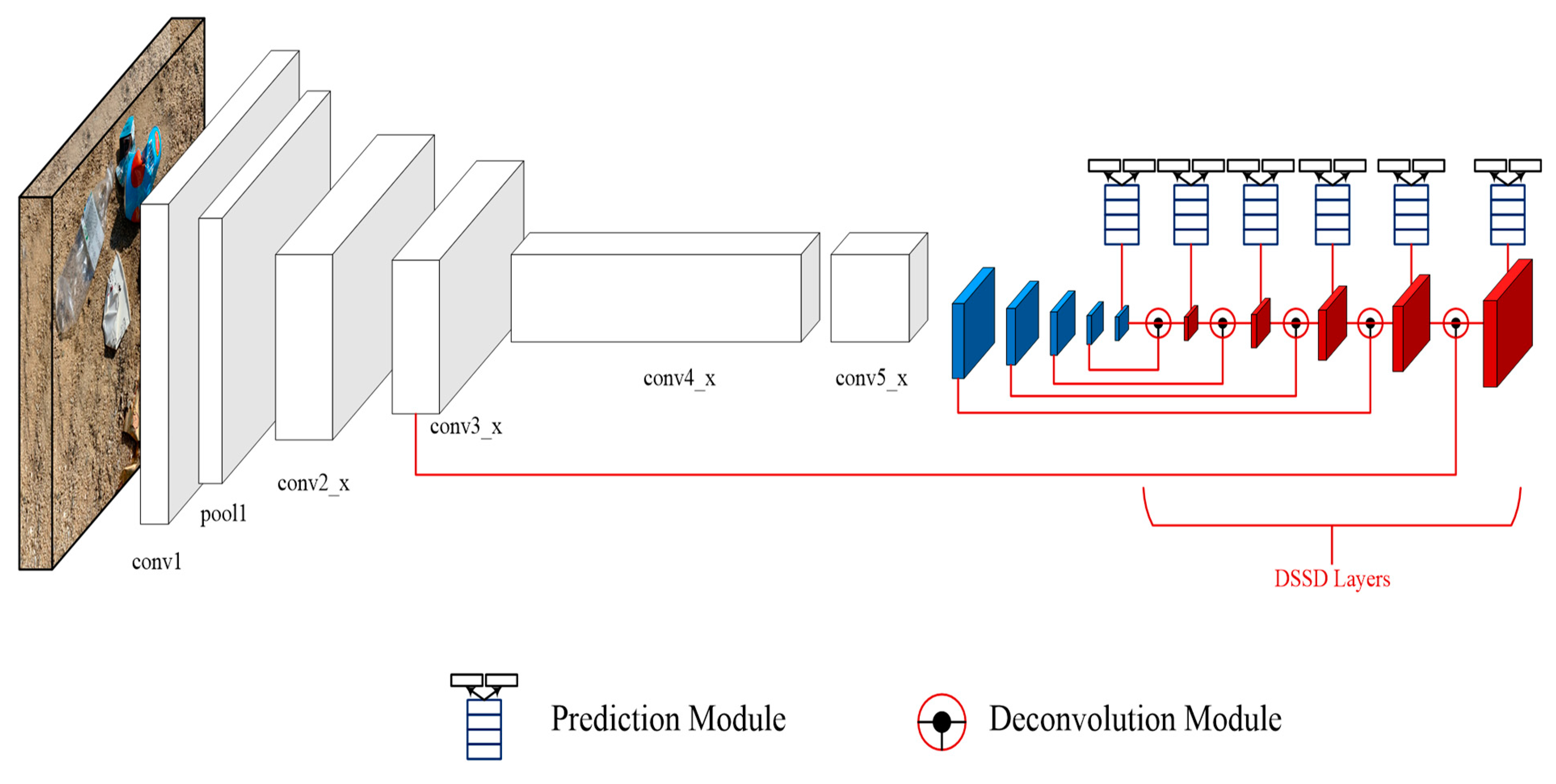
3.3. DSSD
3.4. Limitations of YOLO, SSD, and DSSD
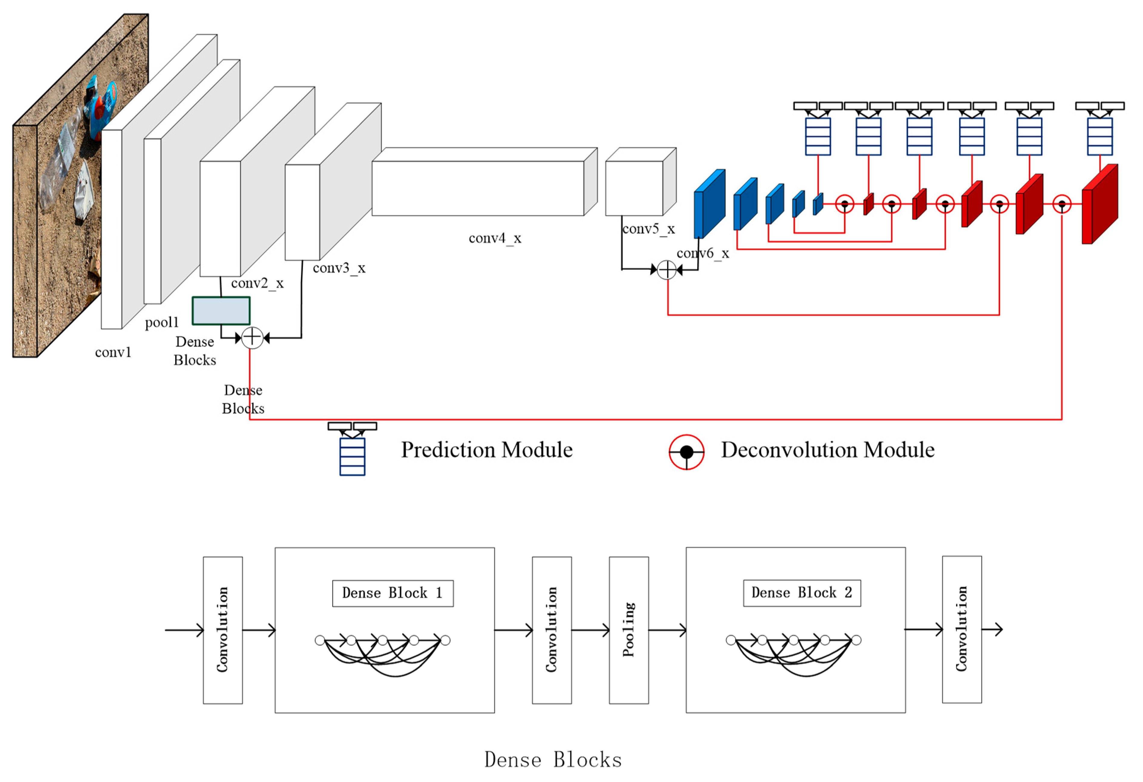
4. Our Approach
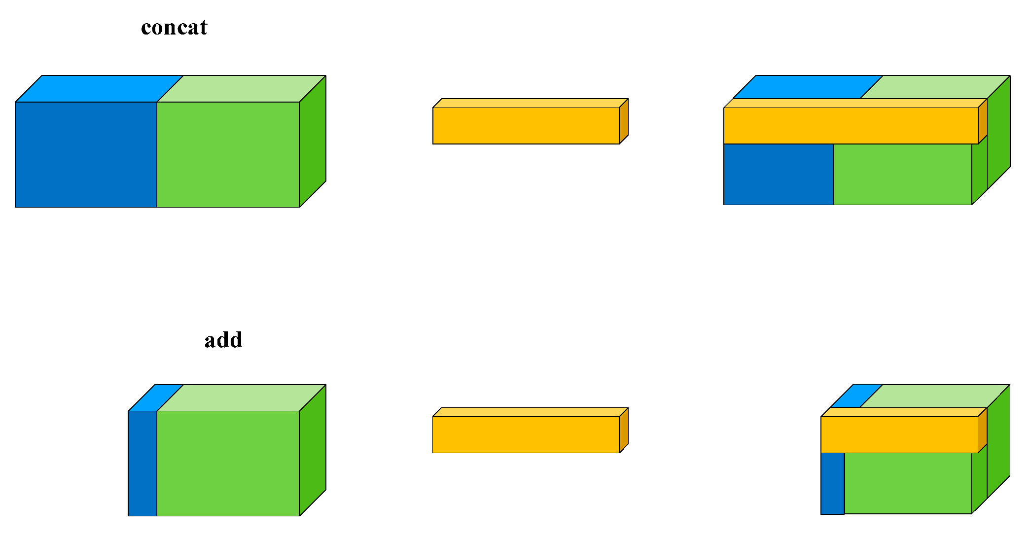
4.1. Context Feature-Fused
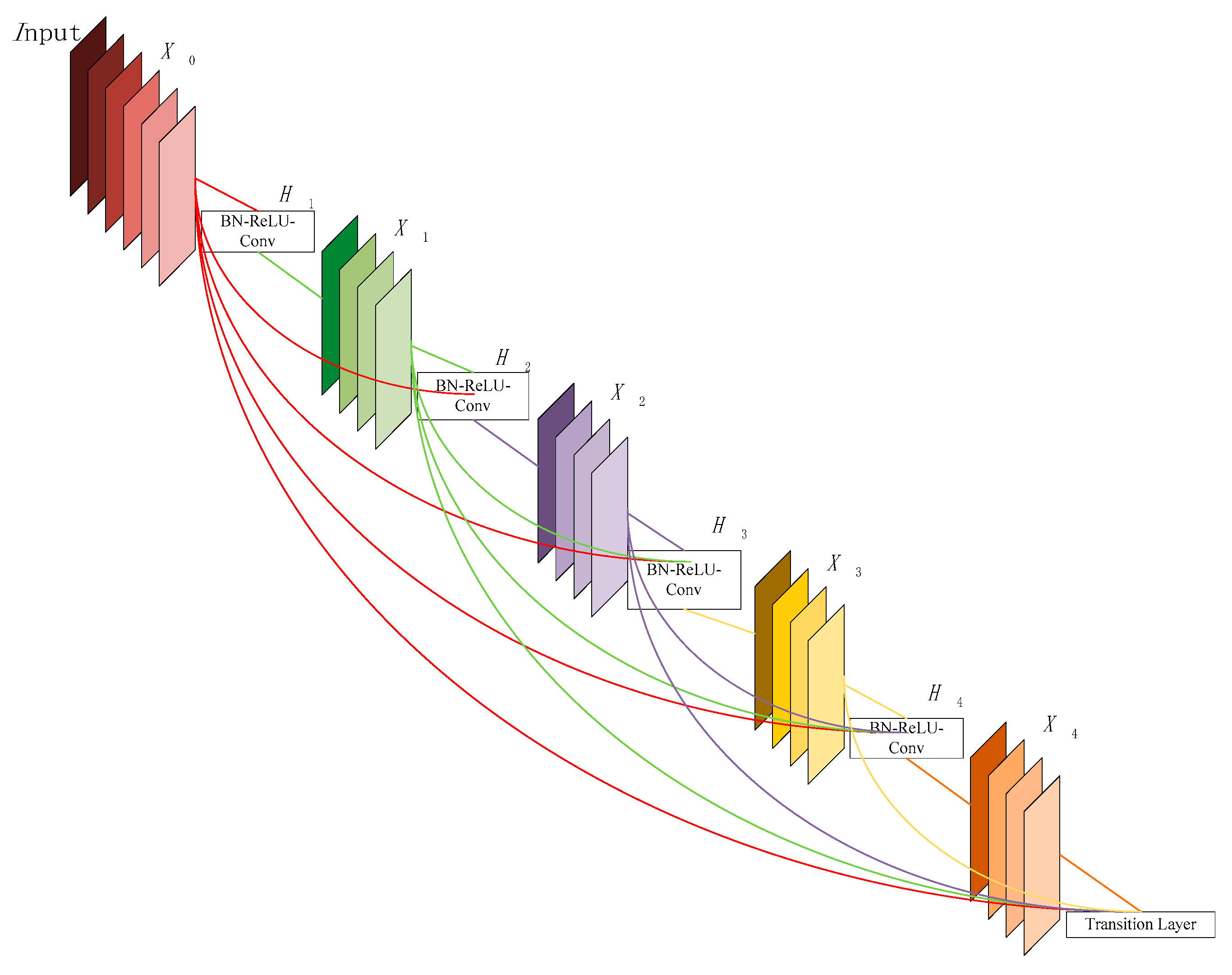
4.2. Dense Block
4.3. Focal Loss
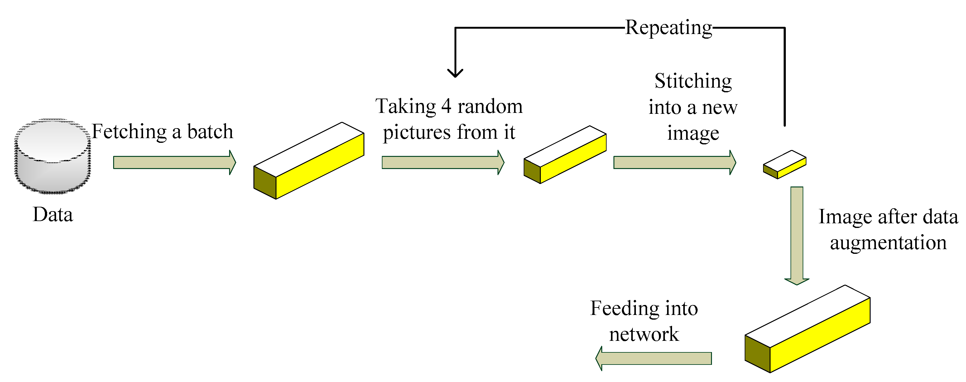
4.4. Mosaic
5. Experiments
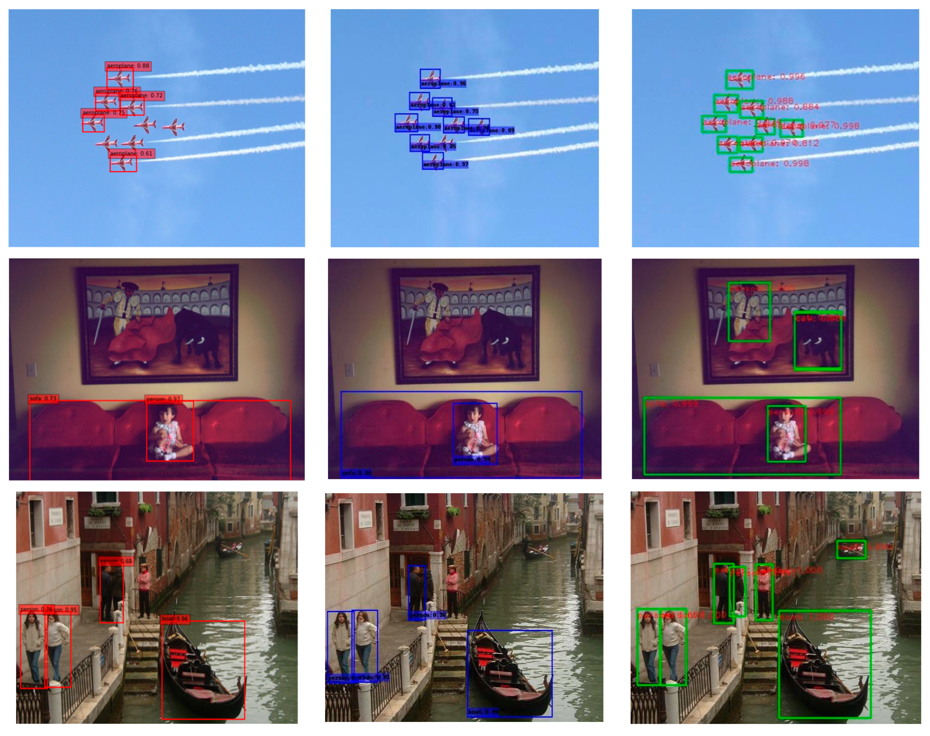
5.1. PASCAL VOC2007
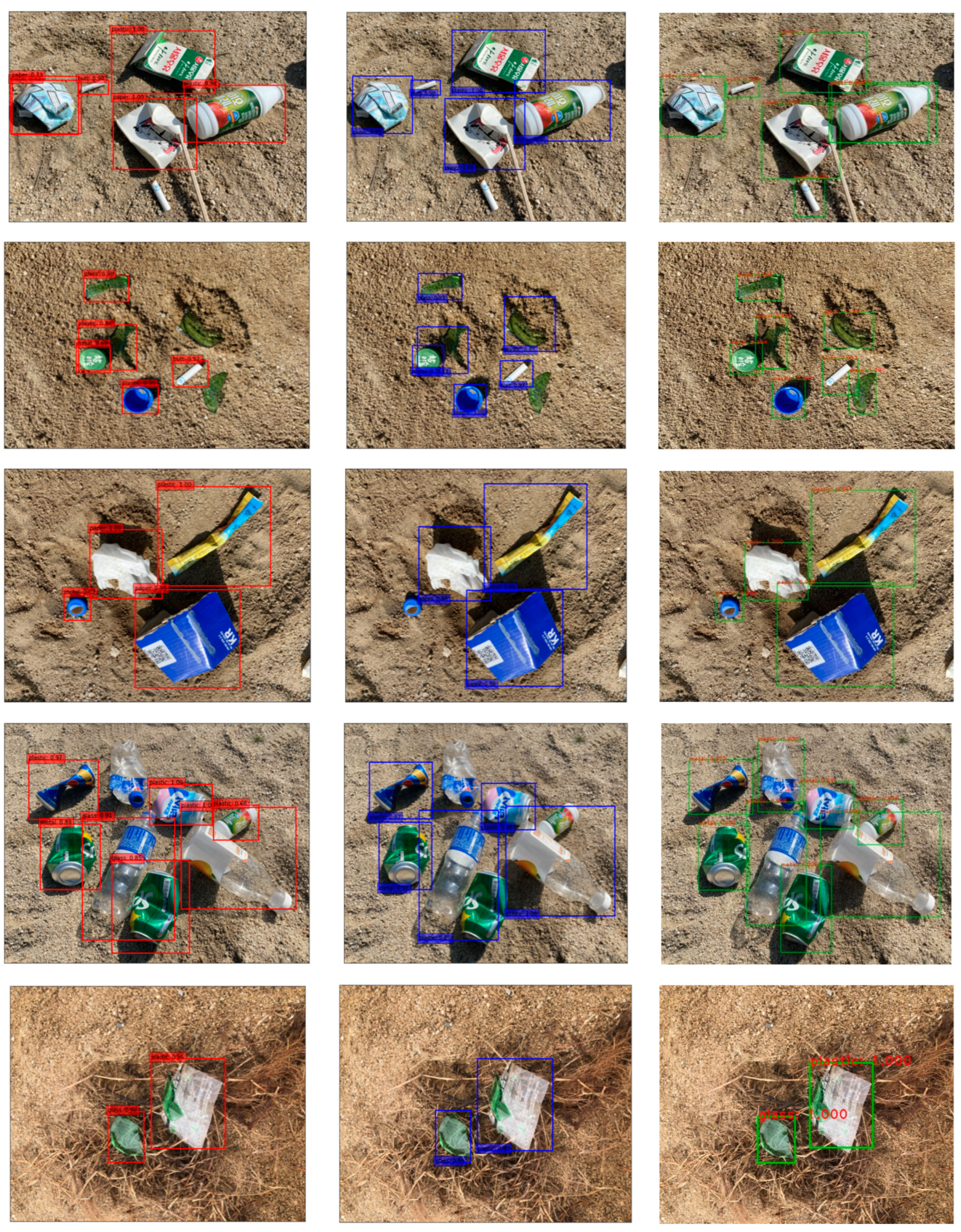
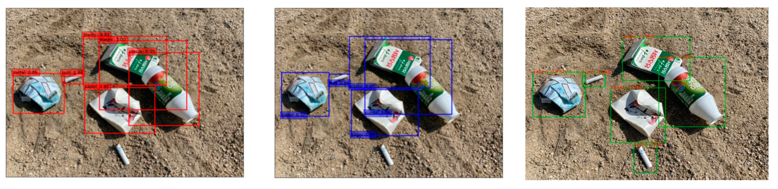
5.2. IST-Waste-V2
6. Conclusions
Author Contributions
Funding
Institutional Review Board Statement
Informed Consent Statement
Data Availability Statement
Conflicts of Interest
References
- Asensio-Montesinos, F.; Anfuso, G.; Williams, A. Beach litter distribution along the western Mediterranean coast of Spain. Mar. Pollut. Bull. 2019, 141, 119–126. [Google Scholar] [CrossRef] [PubMed]
- Nachite, D.; Maziane, F.; Anfuso, G.; Williams, A.T. Spatial and temporal variations of litter at the Mediterranean beaches of Morocco mainly due to beach users. Ocean Coast. Manag. 2019, 179, 104846. [Google Scholar] [CrossRef]
- Willis, K.; Hardesty, B.D.; Vince, J.; Wilcox, C. Local waste management successfully reduces coastal plastic pollution. One Earth. 2022, 6, 666–676. [Google Scholar] [CrossRef]
- Dalal, N.; Triggs, B. Histograms of oriented gradients for human detection. In Proceedings of the 2005 IEEE Computer Society Conference on Computer Vision and Pattern Recognition (CVPR’05), San Diego, CA, USA, 20–25 June 2005; pp. 886–893. [Google Scholar]
- Felzenszwalb, P.; McAllester, D.; Ramanan, D. A discriminatively trained, multiscale, deformable part model. In Proceedings of the 2008 IEEE Conference on Computer Vision and Pattern Recognition, Anchorage, AK, USA, 23–28 June 2008; pp. 1–8. [Google Scholar]
- Girshick, R.; Donahue, J.; Darrell, T.; Malik, J. Rich Feature Hierarchies for Accurate Object Detection and Semantic Segmentation. In Proceedings of the IEEE Conference on Computer Vision and Pattern Recognition, Columbus, OH, USA, 23–28 June 2014; pp. 580–587. [Google Scholar] [CrossRef]
- Girshick, R. Fast r-cnn. In Proceedings of the IEEE International Conference on Computer Vision, Santiago, Chile, 11–18 December 2015; pp. 1440–1448. [Google Scholar]
- Ren, S.; He, K.; Girshick, R.; Sun, J. Faster r-cnn: Towards real-time object detection with region proposal networks. Adv. Neural Inf. Processing Syst. 2015, 28, 91–99. [Google Scholar] [CrossRef]
- Lin, T.-Y.; Dollár, P.; Girshick, R.; He, K.; Hariharan, B.; Belongie, S. Feature pyramid networks for object detection. In Proceedings of the IEEE Conference on Computer Vision and Pattern Recognition, Honolulu, HI, USA, 21–26 July 2017; pp. 2117–2125. [Google Scholar]
- Redmon, J.; Divvala, S.; Girshick, R.; Farhadi, A. You only look once: Unified, real-time object detection. In Proceedings of the IEEE Conference on Computer Vision and Pattern Recognition, Las Vegas, NV, USA, 26 June–1 July 2016; pp. 779–788. [Google Scholar]
- Liu, W.; Anguelov, D.; Erhan, D.; Szegedy, C.; Reed, S.; Fu, C.Y.; Berg, A.C. Ssd: Single shot multibox detector. In European Conference on Computer Vision; Springer: Cham, Switzerland, 2016; pp. 21–37. [Google Scholar]
- Wang, Y.; Wang, C.; Zhang, H.; Dong, Y.; Wei, S. Automatic Ship Detection Based on RetinaNet Using Multi-Resolution Gaofen-3 Imagery. Remote Sens. 2019, 11, 531. [Google Scholar] [CrossRef]
- Ma, W.; Wang, X.; Yu, J. A Lightweight Feature Fusion Single Shot Multibox Detector for Garbage Detection. IEEE Access 2020, 8, 188577–188586. [Google Scholar] [CrossRef]
- Panwar, H.; Gupta, P.; Siddiqui, M.K.; Morales-Menendez, R.; Bhardwaj, P.; Sharma, S.; Sarker, I.H. AquaVision: Automating the detection of waste in water bodies using deep transfer learning. Case Stud. Chem. Environ. Eng. 2020, 2, 100026. [Google Scholar] [CrossRef]
- Shi, C.; Xia, R.; Wang, L. A Novel Multi-Branch Channel Expansion Network for Garbage Image Classification. IEEE Access 2020, 8, 154436–154452. [Google Scholar] [CrossRef]
- Toğaçar, M.; Ergen, B.; Cömert, Z. Waste classification using AutoEncoder network with integrated feature selection method in convolutional neural network models. Measurement 2020, 153, 107459. [Google Scholar] [CrossRef]
- Yi, H.S.; Chellappan, S. Computer Vision Assisted Approaches to Detect Street Garbage from Citizen Generated Imagery. In International Summit Smart City 360°; Springer: Cham, Switzerland, 2021; pp. 526–541. [Google Scholar]
- Nazerdeylami, A.; Majidi, B.; Movaghar, A. Autonomous litter surveying and human activity monitoring for governance intelligence in coastal eco-cyber-physical systems. Ocean Coast. Manag. 2021, 200, 105478. [Google Scholar] [CrossRef]
- Kraft, M.; Piechocki, M.; Ptak, B.; Walas, K. Autonomous, Onboard Vision-Based Trash and Litter Detection in Low Altitude Aerial Images Collected by an Unmanned Aerial Vehicle. Remote Sens. 2021, 13, 965. [Google Scholar] [CrossRef]
- Li, J.; Liang, X.; Shen, S.; Xu, T.; Feng, J.; Yan, S. Scale-aware Fast R-CNN for Pedestrian Detection. IEEE Trans. Multimed. 2017, 20, 985–996. [Google Scholar] [CrossRef]
- He, K.; Zhang, X.; Ren, S.; Sun, J. Spatial pyramid pooling in deep convolutional networks for visual recognition. In IEEE Transactions on Pattern Analysis and Machine Intelligence; IEEE: Piscataway, NJ, USA, 2015; Volime 37, pp. 1904–1916. [Google Scholar]
- Mnih, V.; Heess, N.; Graves, A. Recurrent models of visual attention. Adv. Neural Inf. Processing Syst. 2014, 27, 2204–2212. [Google Scholar]
- Larochelle, H.; Hinton, G.E. Learning to combine foveal glimpses with a third-order Boltzmann machine. Adv. Neural Inf. Processing Syst. 2010, 23, 1243–1251. [Google Scholar]
- Chen, L.-C.; Yang, Y.; Wang, J.; Xu, W.; Yuille, A.L. Attention to scale: Scale-aware semantic image segmentation. In Proceedings of the IEEE Conference on Computer Vision and Pattern Recognition, Las Vegas, NV, USA, 26 June–1 July 2016; pp. 3640–3649. [Google Scholar]
- Gregor, K.; Danihelka, I.; Graves, A.; Rezende, D.; Wierstra, D. Draw: A recurrent neural network for image generation. In Proceedings of the 32nd International Conference on Machine Learning, PMLR, Lille, France, 6–11 July 2015; pp. 1462–1471. [Google Scholar]
- Fu, C.Y.; Liu, W.; Ranga, A.; Tyagi, A.; Berg, A.C. Dssd: Deconvolutional single shot detector. arXiv 2017, arXiv:1701.06659. [Google Scholar]
- Redmon, J.; Farhadi, A. YOLO9000: Better, faster, stronger. In Proceedings of the IEEE Conference on Computer Vision and Pattern Recognition, Honolulu, HI, USA, 21–26 July 2017; pp. 7263–7271. [Google Scholar]
- Sermanet, P.; Eigen, D.; Zhang, X.; Mathieu, M.; Fergus, R.; LeCun, Y. Overfeat: Integrated recognition, localization and detection using convolutional networks. arXiv 2013, arXiv:1312.6229. [Google Scholar]
- Lin, T.-Y.; Goyal, P.; Girshick, R.; He, K.; Dollár, P. Focal loss for dense object detection. In Proceedings of the IEEE Conference on Computer Vision and Pattern Recognition, Honolulu, HI, USA, 21–26 July 2017; pp. 2980–2988. [Google Scholar]
- Teichmann, M.; Weber, M.; Zollner, M.; Cipolla, R.; Urtasun, R. MultiNet: Real-time Joint Semantic Reasoning for Autonomous Driving. In Proceedings of the 2018 IEEE Intelligent Vehicles Symposium (IV), Changshu, China, 26–30 June 2018; pp. 1013–1020. [Google Scholar]
- Quan, T.M.; Hilderbrand, D.G.C.; Jeong, W. FusionNet: A deep fully residual convolutional neural network for image segmentation in connectomics. arXiv 2016, arXiv:1612.05360. [Google Scholar] [CrossRef]

| Method | mAP | Bike | Aero | Bird | Boat | Bottle | Bus | Car | Cat | Chair | Cow |
|---|---|---|---|---|---|---|---|---|---|---|---|
| Faster R-CNN | 76.4 | 80.7 | 79.8 | 76.2 | 68.3 | 55.9 | 85.1 | 85.3 | 89.8 | 56.7 | 87.8 |
| SSD321 | 77.1 | 76.3 | 84.6 | 79.3 | 64.6 | 47.2 | 85.4 | 84.0 | 88.8 | 60.1 | 81.5 |
| DSSD321 | 78.6 | 81.9 | 84.9 | 80.5 | 68.4 | 53.9 | 85.6 | 86.2 | 88.9 | 61.1 | 82.6 |
| DSSD513 | 81.5 | 86.2 | 86.6 | 82.6 | 74.9 | 62.5 | 89.0 | 88.7 | 88.8 | 65.2 | 87.0 |
| MS-DSSD 321 | 80.3 | 83.1 | 84.6 | 82.5 | 70.2 | 57.6 | 89.1 | 88.2 | 87.9 | 63.8 | 85.2 |
| MS-DSSD 513 | 82.2 | 87.8 | 86.9 | 84.1 | 76.5 | 66.1 | 89.2 | 88.5 | 89.0 | 66.9 | 87.5 |
| Method | mAP | table | dog | horse | mbike | person | plant | sheep | sofa | train | tv |
| Faster R-CNN | 76.4 | 69.4 | 87.2 | 88.9 | 80.9 | 78.4 | 41.7 | 78.6 | 79.8 | 85.3 | 72.0 |
| SSD321 | 77.1 | 76.9 | 86.7 | 87.2 | 85.4 | 79.1 | 50.8 | 77.2 | 82.6 | 87.3 | 76.6 |
| DSSD321 | 78.6 | 78.7 | 86.7 | 88.7 | 86.7 | 79.7 | 51.7 | 78.0 | 80.9 | 87.2 | 79.4 |
| DSSD513 | 81.5 | 78.7 | 88.2 | 89.0 | 87.5 | 83.7 | 51.1 | 86.3 | 81.6 | 85.7 | 83.7 |
| MS-DSSD 321 | 80.3 | 78.9 | 87.6 | 89.2 | 87.1 | 83.7 | 52.6 | 84.2 | 81.1 | 87.3 | 81.9 |
| MS-DSSD 513 | 82.2 | 78.4 | 87.9 | 89.9 | 88.8 | 84.8 | 54.3 | 86.1 | 82.0 | 85.4 | 82.9 |
| No | Classes | Number of Images |
|---|---|---|
| 1 | Plastic | 4789 |
| 2 | Metal | 405 |
| 3 | Paper | 1740 |
| 4 | Cigarette Butts | 389 |
| 5 | Wood | 429 |
| 6 | Glass | 254 |
| Method | mAP | Plastic | Metal | Paper | Butt | Wood | Glass |
|---|---|---|---|---|---|---|---|
| Faster R-CNN (VGG) | 79.8 | 88.1 | 85.4 | 88.3 | 67.6 | 59.8 | 89.5 |
| SSD321 | 80.1 | 89.1 | 85.3 | 88.9 | 61.5 | 67.1 | 92.9 |
| DSSD321 | 81.2 | 87.7 | 86.1 | 88.4 | 70.2 | 62.1 | 92.7 |
| DSSD513 | 81.5 | 88.4 | 86.6 | 87.5 | 71.2 | 61.8 | 93.3 |
| MS-DSSD 321 | 82.3 | 89.5 | 88.2 | 89.6 | 73.7 | 62.1 | 93.8 |
| MS-DSSD 513 | 84.1 | 91.5 | 89.0 | 91.2 | 73.9 | 63.8 | 95.2 |
Publisher’s Note: MDPI stays neutral with regard to jurisdictional claims in published maps and institutional affiliations. |
© 2022 by the authors. Licensee MDPI, Basel, Switzerland. This article is an open access article distributed under the terms and conditions of the Creative Commons Attribution (CC BY) license (https://creativecommons.org/licenses/by/4.0/).
Share and Cite
Ren, C.; Lee, S.; Kim, D.-K.; Zhang, G.; Jeong, D. A Multi-Strategy Framework for Coastal Waste Detection. J. Mar. Sci. Eng. 2022, 10, 1330. https://doi.org/10.3390/jmse10091330
Ren C, Lee S, Kim D-K, Zhang G, Jeong D. A Multi-Strategy Framework for Coastal Waste Detection. Journal of Marine Science and Engineering. 2022; 10(9):1330. https://doi.org/10.3390/jmse10091330
Chicago/Turabian StyleRen, Chengjuan, Sukhoon Lee, Dae-Kyoo Kim, Guangnan Zhang, and Dongwon Jeong. 2022. "A Multi-Strategy Framework for Coastal Waste Detection" Journal of Marine Science and Engineering 10, no. 9: 1330. https://doi.org/10.3390/jmse10091330
APA StyleRen, C., Lee, S., Kim, D.-K., Zhang, G., & Jeong, D. (2022). A Multi-Strategy Framework for Coastal Waste Detection. Journal of Marine Science and Engineering, 10(9), 1330. https://doi.org/10.3390/jmse10091330