
Underwater Anthropogenic Noise Pollution Assessment in Shallow Waters on the South-Eastern Coast of Spain


Abstract
1. Introduction
2. Materials and Methods
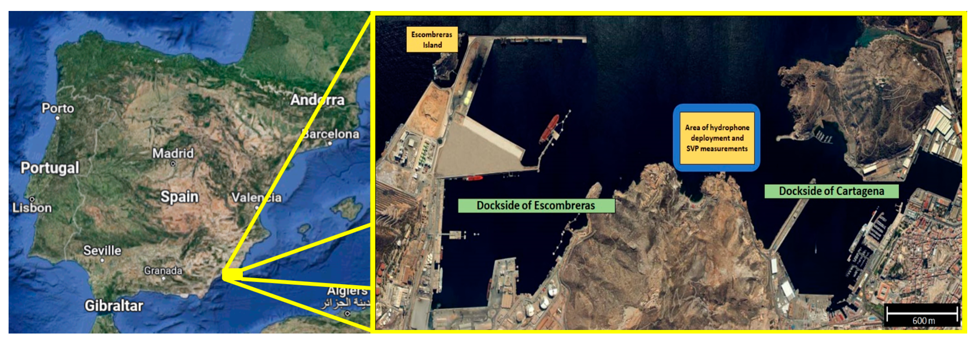
2.1. Study Area
2.2. Marine Traffic Monitoring
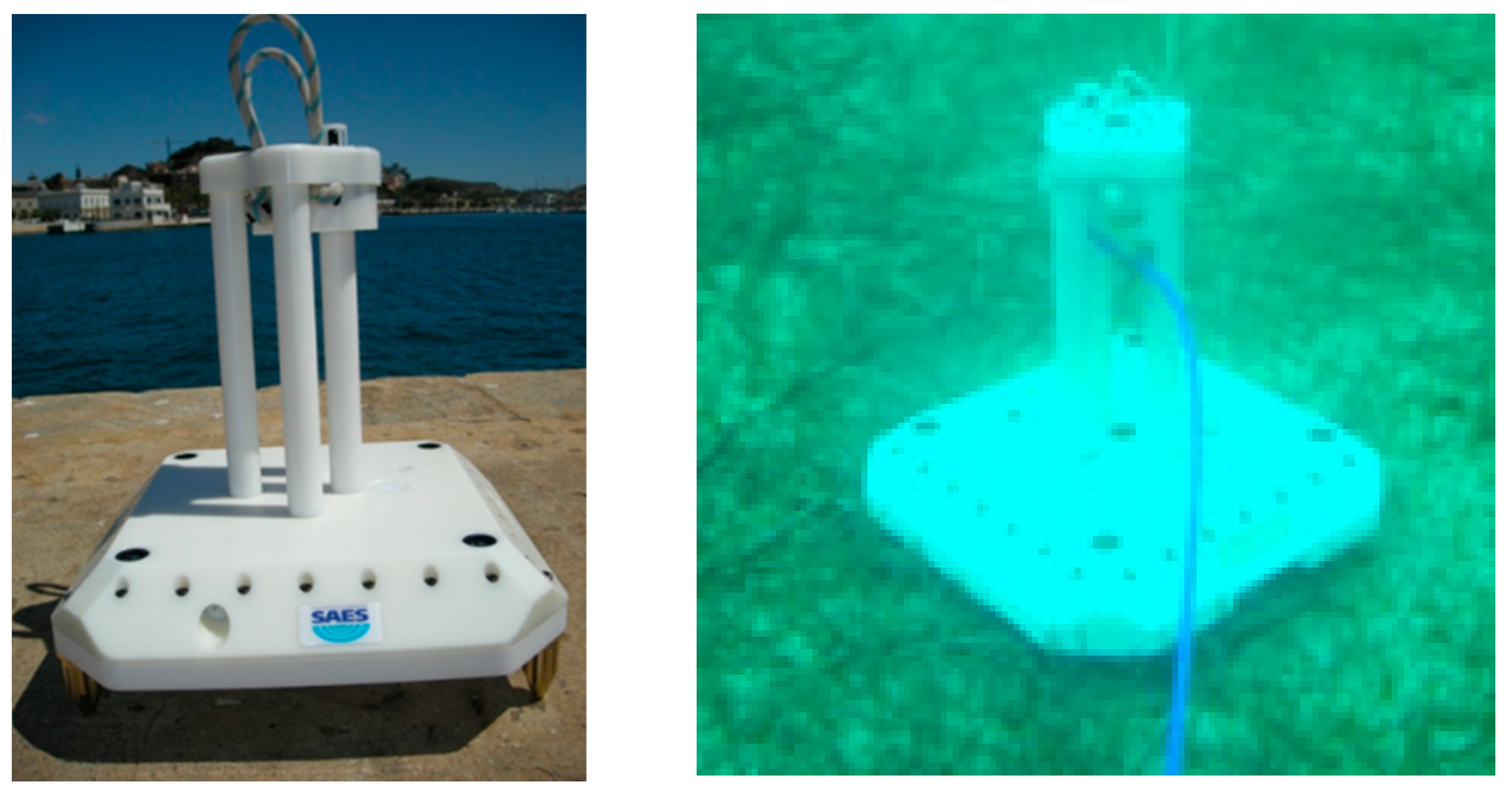
2.3. Data Measurement
2.4. Classification of the Measurements
2.5. Acoustic Data Analysis
2.6. Statistical Analysis
3. Results
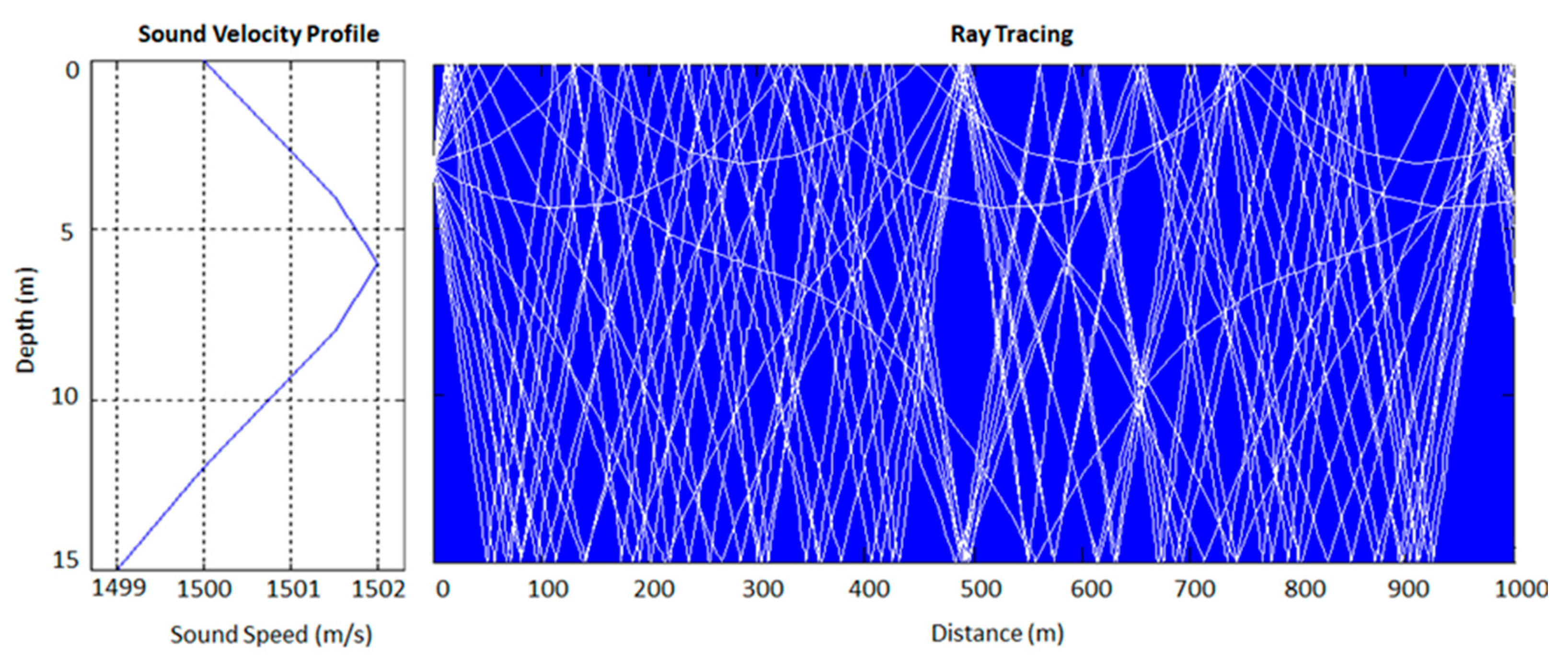
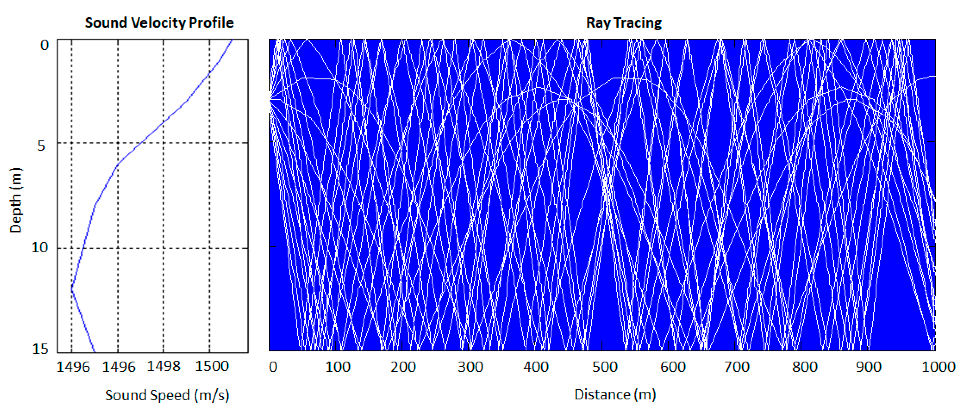
3.1. Sound Velocity Profile and Sound Scattering Estimations
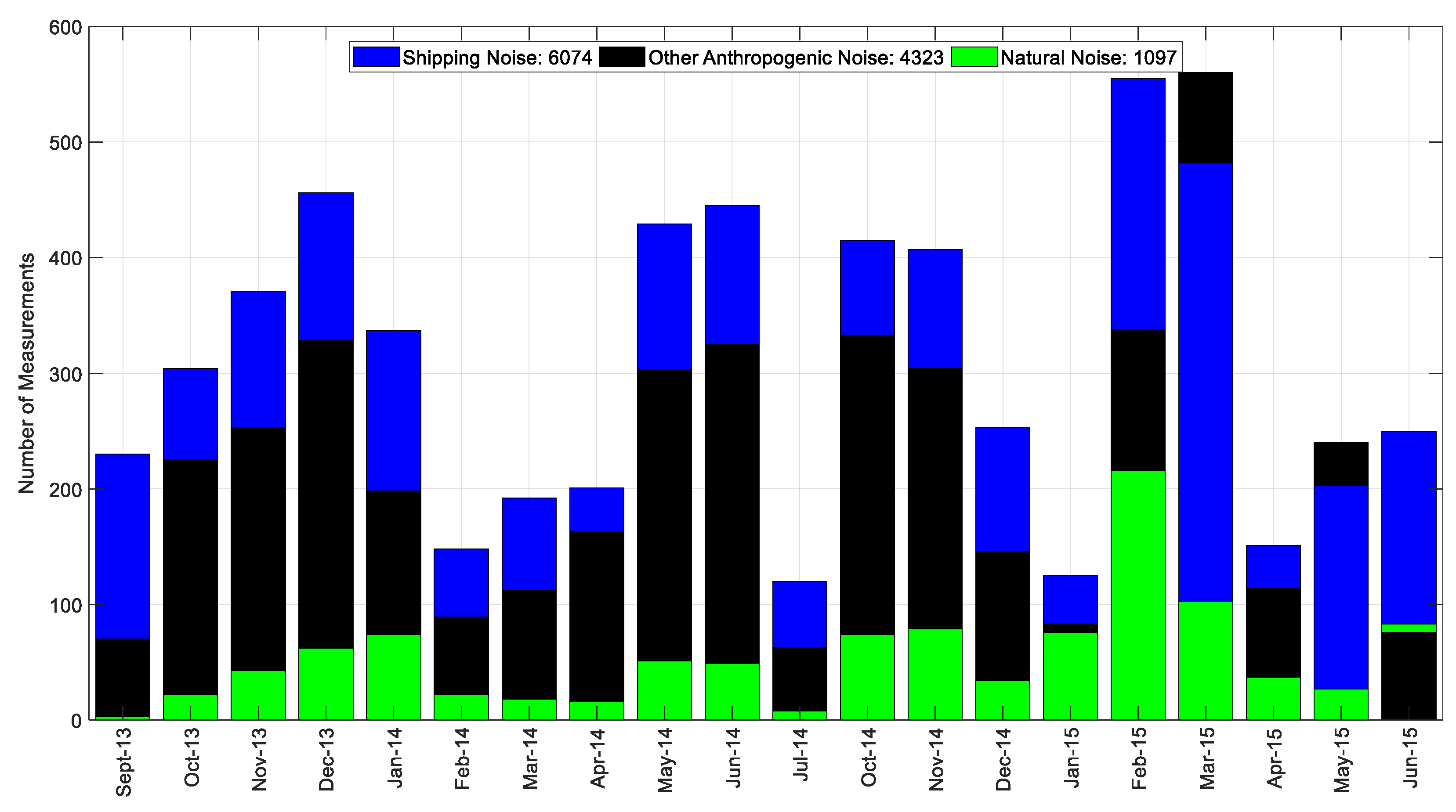
3.2. Classification of the Measurements
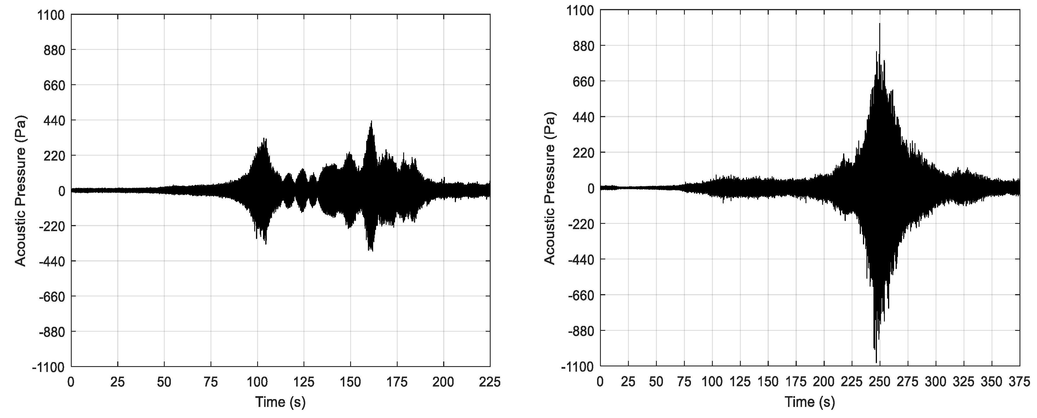
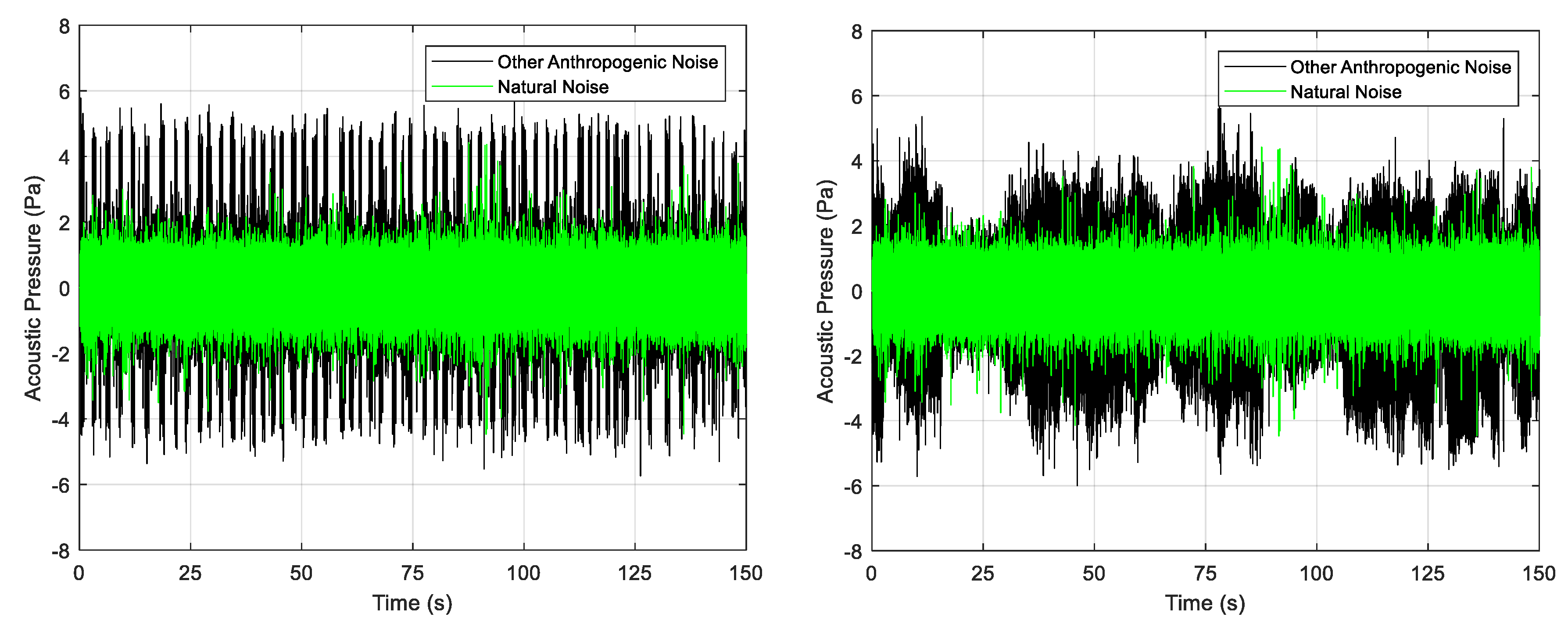
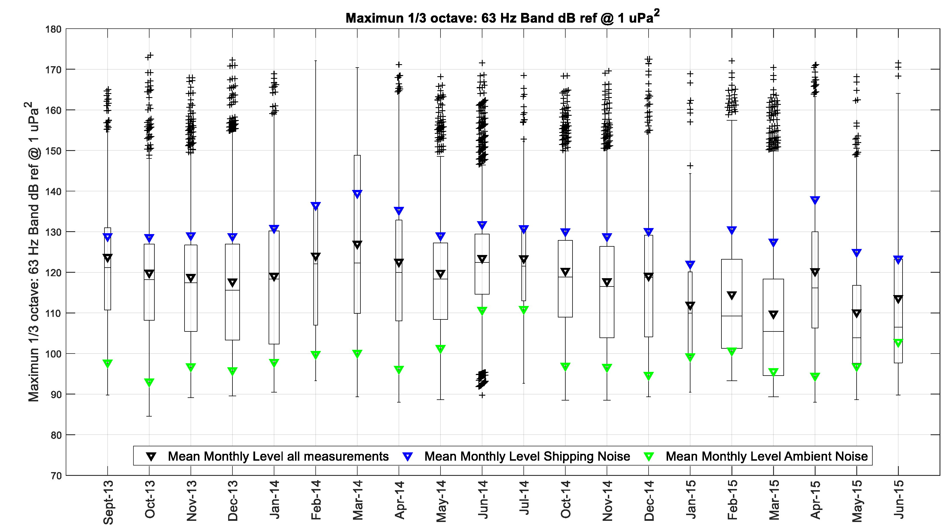
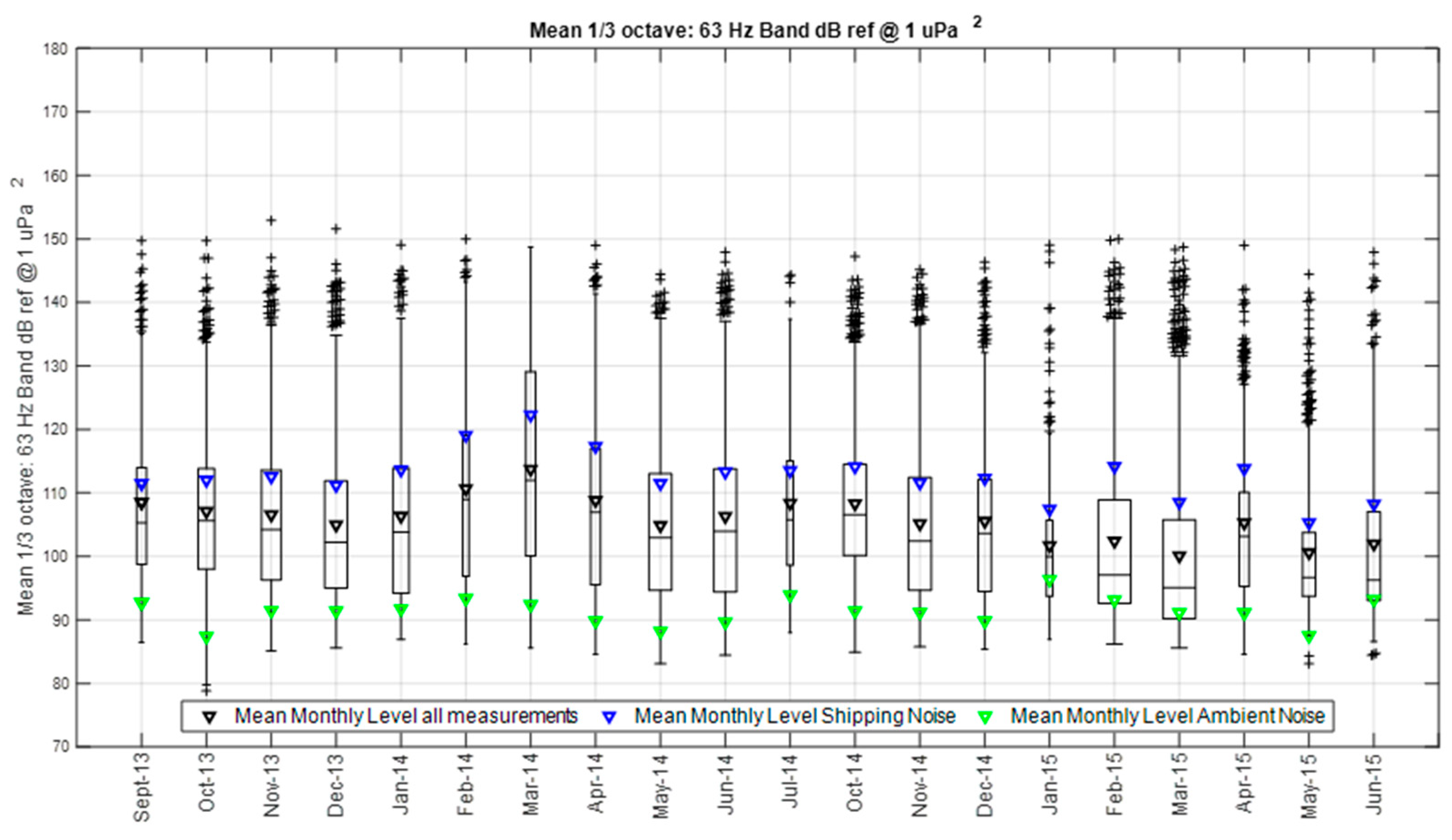
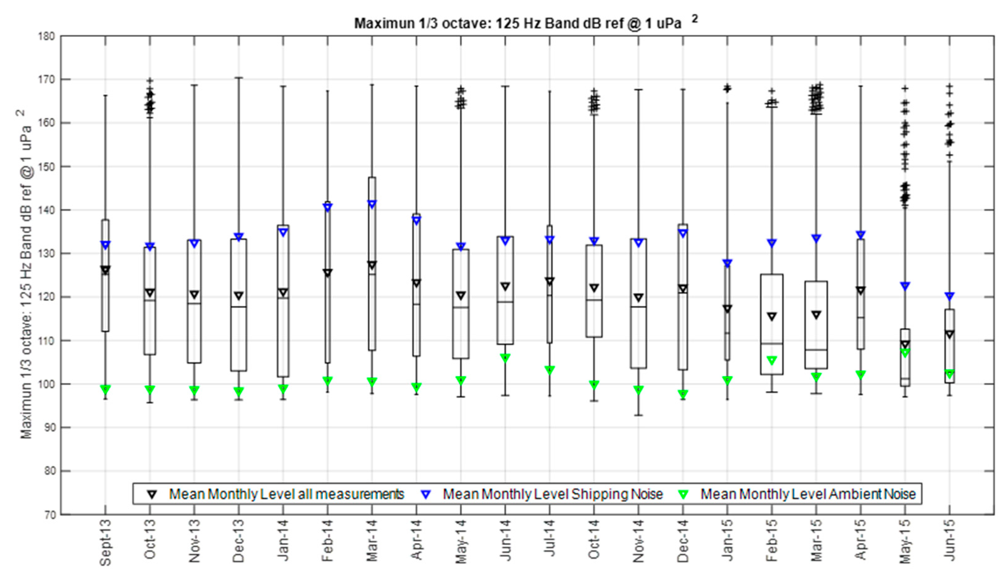
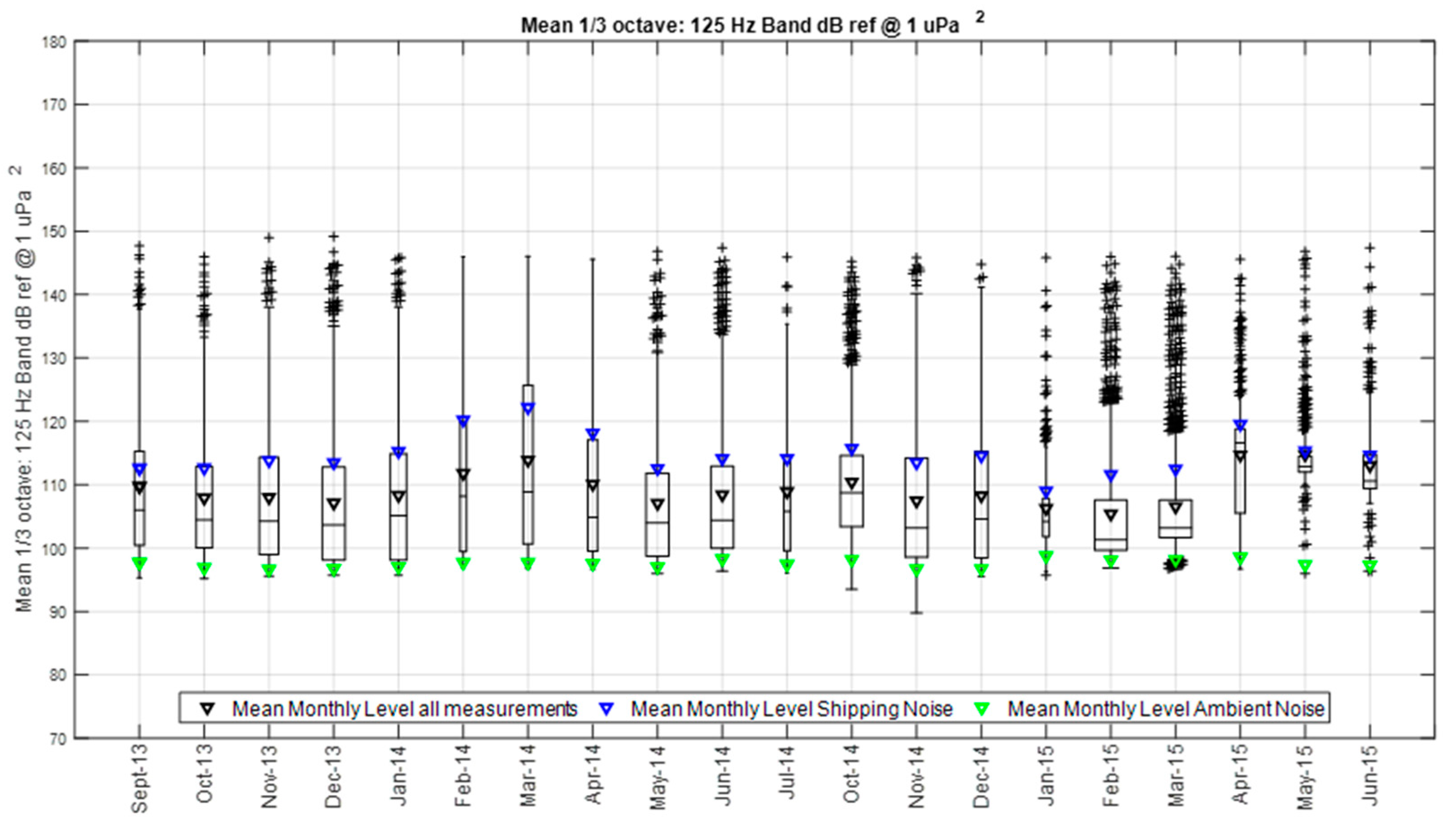
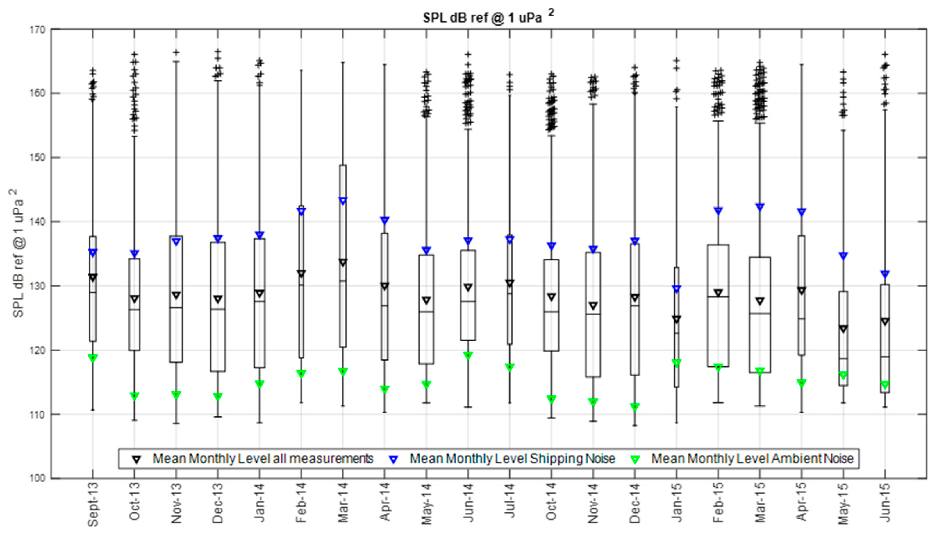
3.3. Acoustic Analysis
4. Discussion
5. Conclusions
- In the study area, the noise levels are higher than the levels recommended in order to achieve good environmental status; therefore, mitigation policies are needed to control ship traffic and the underwater radiated noise it produces.
- Underwater radiated noise caused by ships must be regulated, controlled and standardized by shipyards in addition to the use of Spatio-Temporal Restrictions (STRs).
- The European Directive [61] must be extended to small ships in order to control the traffic of recreational and small ships.
- It is recommended to increase the analyzed acoustic bandwidth and include additional 1/3 octave bands in studies of underwater acoustic pollution and its impact on the maritime ecosystem.
Author Contributions
Funding
Institutional Review Board Statement
Informed Consent Statement
Data Availability Statement
Acknowledgments
Conflicts of Interest
References
- Wenz, G.M. Acoustic ambient noise in the ocean: Spectra and sources. J. Acoust. Soc. Am. 1962, 34, 1936–1956. [Google Scholar] [CrossRef]
- Richardson, W.J.; Greene, C.R., Jr.; Malme, C.I.; Thomson, D.H. Marine Mammals and Noise; Academic: New York, NY, USA, 1995; ISBN 9780125884419. [Google Scholar]
- Robinson, S.P.; Lepper, P.A.; Hazelwood, R.A. Good Practice Guide for Underwater Noise Measurement; NPL Good Practice Guide No. 133; National Measurement Office: London, UK; Marine Scotland: Edinburgh, Scotland; The Crown Estate: London, UK, 2014; ISSN 1368-6550. [Google Scholar]
- Hildebrand, J.A. Anthropogenic and natural sources of ambient noise in the ocean. Mar. Ecol. Prog. Ser. 2009, 395, 5–20. [Google Scholar] [CrossRef]
- Urick, R.J. Principles of Underwater Sound, 3rd ed.; McGraw-Hill: New York, NY, USA, 1983. [Google Scholar]
- Farina, A. Soundscape Ecology: Principles, Patterns, Methods and Applications; Springer: Berlin/Heidelberg, Germany, 2014. [Google Scholar] [CrossRef]
- Dekeling, R.P.A.; Tasker, M.L.; Van der Graaf, A.J.; Ainslie, M.A.; Andersson, M.H.; André, M.; Borsani, J.F.; Brensing, K.; Castellote, M.; Cronin, D.; et al. Monitoring Guidance for Underwater Noise in European Seas; Part II: Monitoring Guidance Specifications, JRC Scientific and Policy Report EUR 26555 EN; Publications Office of the European Union: Luxembourg, 2014. [Google Scholar] [CrossRef]
- Mitson, R.B.; Knudsen, H.P. Causes and effects of underwater noise on fish abundance estimation. Aquat. Living Resour. 2003, 16, 255–263. [Google Scholar] [CrossRef]
- Ross, D. Mechanics of Underwater Noise; Peninsula Publishing: Los Altos, CA, USA, 1987; ISBN 9780932146168. [Google Scholar]
- Ross, D. On ocean underwater ambient noise. Inst. Acoust. Bull. 1993, 18, 5–8. [Google Scholar]
- Ross, D. Ship sources of ambient noise. IEEE J. Ocean. Eng. 2005, 30, 257–261. [Google Scholar] [CrossRef]
- Bjorno, L. Man-made contributions to ambient noise in the seas. In Proceedings of the fourth European Conference on Underwater Acoustics 2; Alippi, A., Cannelli, G.B., Eds.; CNR-IDAC: Rome, Italy, 1998; pp. 543–548. [Google Scholar]
- Andrew, R.K.; Howe, B.M.; Mercer, J.A.; Dzieciuch, M.A. Ocean ambient sound: Comparing the 1960s with the 1990s for a receiver off the California coast. Acoust. Res. Lett. Online 2002, 3, 65–70. [Google Scholar] [CrossRef]
- Mazzuca, L.L. Potential Effects of Low Frequency Sound (LFS) from Commercial Vessels on Large Whales. Master Thesis, University of Washington, Seattle, WA, USA, 2001. [Google Scholar]
- McDonald, M.A.; Hildebrand, J.A.; Wiggins, S.M. Increases in deep ocean ambient noise in the Northeast Pacific west of San Nicolas Island, California. J. Acoust. Soc. Am. 2006, 120, 711–718. [Google Scholar] [CrossRef]
- Chapman, N.R.; Price, A. Low frequency deep ocean ambient noise trend in the Northeast Pacific Ocean. J. Acoust. Soc. Am. 2011, 129, EL161–EL165. [Google Scholar] [CrossRef]
- Hildebrand, J.A. Sources of Anthropogenic Sound in the Marine Environment. International Policy Workshop on Sound and Marine Mammals, London, UK, 28–30 September. 2004. Available online: https://www.mmc.gov/wp-content/uploads/hildebrand.pdf (accessed on 16 July 2022).
- McDonald, M.A.; Hildebrand, J.A.; Wiggins, S.M.; Ross, D. A 50 year comparison of ambient noise in Northeast Pacific west of San Nicolas Island, California. J. Acoust. Soc. Am. 2008, 124, 1985–1992. [Google Scholar] [CrossRef]
- Merchant, N.D.; Witt, M.J.; Blondel, P.; Godley, B.J.; Smith, G.H. Assessing sound exposure from shipping in coastal waters using a single hydrophone and automatic identification system (AIS) data. Mar. Pollut. Bull. 2012, 64, 1320–1329. [Google Scholar] [CrossRef]
- OSPAR Commission. Overview of the Impacts of Anthropogenic Underwater Sound in the Marine Environment; Report, 441; OSPAR Commission: London, UK, 2009. [Google Scholar]
- Frisk, G.V. Noiseonomics: The relationship between ambient noise levels in the sea and global economic trends. Sci. Rep. 2012, 2, 437. [Google Scholar] [CrossRef] [PubMed]
- Lesage, V.; Barrette, C.; Kingsley, M.; Sjare, B. The effect of vessel noise on the vocal behaviour of belugas in the St. Lawrence River estuary, Canada. Mar. Mammal Sci. 1999, 15, 65–84. [Google Scholar] [CrossRef]
- Finneran, J.J.; Schlundt, C.E.; Dear, R.; Carder, D.A.; Ridgway, S.H. Temporary shift in masked hearing thresholds in odontocetes after exposure to single underwater impulses from a seismic watergun. J. Acoust. Soc. Am. 2002, 111, 2929–2940. [Google Scholar] [CrossRef] [PubMed]
- Janik, V.M. Underwater acoustic communication networks in marine mammals. In Animal Communication Networks; McGregor, P.K., Ed.; Cambridge University Press: Cambridge, UK, 2005; pp. 390–415. [Google Scholar] [CrossRef]
- Madsen, P.T.; Wahlberg, M.; Tougaard, J.; Lucke, K.; Tyack, P. Wind turbine underwater noise and marine mammals: Implications of current knowledge and data needs. Mar. Ecol. Prog. Ser. 2006, 309, 279–295. [Google Scholar] [CrossRef]
- Lucke, K.; Lepper, P.A.; Hoeve, B.; Everaarts, E.; van Elk, N.; Siebert, U. Perception of low-frequency acoustic signals by a harbour porpoise (Phocoena phocoena) in the presence of simulated offshore wind turbine noise. Aquat. Mamm. 2007, 33, 55–68. [Google Scholar] [CrossRef]
- Clark, C.W.; Ellison, W.T.; Southall, B.L.; Hatch, L.; Van Parijs, S.M.; Frankel, A.; Ponirakis, D. Acoustic masking in marine ecosystems: Intuitions, analysis, and implication. Mar. Ecol. Prog. Ser. 2009, 395, 201–222. [Google Scholar] [CrossRef]
- Holles, S.; Simpson, S.D.; Radford, A.N.; Berten, L.; Lecchini, D. Boat noise disrupts orientation behaviour in a coral reef fish. Mar. Ecol. Prog. Ser. 2013, 485, 295–300. [Google Scholar] [CrossRef]
- Wysocki, L.E.; Dittami, J.P.; Ladich, F. Ship noise and cortisol secretion in European freshwater fishes. Biol. Conserv. 2006, 128, 501–508. [Google Scholar] [CrossRef]
- Southall, B.L.; Bowles, A.E.; Ellison, W.T.; Finneran, J.J.; Gentry, R.L.; Greene, C.R.; Kastak, D.; Ketten, D.R.; Miller, J.H.; Nachtigall, P.E.; et al. Marine mammal noise exposure criteria: Initial scientific recommendations. Aquat. Mamm. 2007, 33, 4. [Google Scholar] [CrossRef]
- Codarin, A.; Wysocki, L.E.; Ladich, F.; Picciulin, M. Effects of ambient and boat noise on hearing and communication in three fish species living in a marine protected area (Miramare, Italy). Mar. Pollut. Bull. 2009, 58, 1880–1887. [Google Scholar] [CrossRef]
- Popper, A.N.; Hastings, M.C. The effects of anthropogenic sources of sound on fishes. J. Fish Biol. 2009, 75, 455–489. [Google Scholar] [CrossRef] [PubMed]
- Rolland, R.M.; Parks, S.E.; Hunt, K.E.; Castellote, M.; Corkeron, P.J.; Nowacek, D.P.; Wasser, S.K.; Kraus, S.D. Evidence that ship noise increases stress in right whales. Proc. R. Soc. B Biol. Sci. 2012, 279, 2363–2368. [Google Scholar] [CrossRef] [PubMed]
- Miller, P.; Biassoni, N.; Samuels, A.; Tyack, P. Whale songs lengthen in response to sonar. Nature 2000, 405, 903. [Google Scholar] [CrossRef] [PubMed]
- Slabbekoorn, H.; Bouton, N.; van Opzeeland, I.; Coers, A.; ten Cate, C.; Popper, A. A noisy spring: The impact of globally rising underwater sound levels on fish. Trends Ecol. Evol. 2010, 25, 419–427. [Google Scholar] [CrossRef]
- André, M.; van der Schaar, M.; Zaugg, S.; Houégnigan, L.; Sánchez, A.; Castell, J. Listening to the deep: Live monitoring of ocean noise and cetacean acoustic signals. Mar. Pollut. Bull. 2011, 63, 18–26. [Google Scholar] [CrossRef]
- Castellote, M.; Clark, C.W.; Lammers, M.O. Acoustic and behavioural changes by fin whales (Balaenoptera physalus) in response to shipping and airgun noise. Biol. Conserv. 2012, 147, 115–122. [Google Scholar] [CrossRef]
- Fewtrell, J.; McCauley, R. Impact of air gun noise on the behaviour of marine fish and squid. Mar. Pollut. Bull. 2012, 64, 984–993. [Google Scholar] [CrossRef]
- Dyndo, M.; Wisniewska, D.M.; Rojano-Donate, L.; Madsen, P.T. Harbour porpoises react to low levels of high frequency vessel noise. Sci. Rep. 2015, 5, 11083. [Google Scholar] [CrossRef]
- Gomez, C.; Lawson, J.; Wright, A.J.; Buren, A.; Tollit, D.; Lesage, V. A systematic review on the behavioural responses of wild marine mammals to noise: The disparity between science and policy. Can. J. Zool. 2016, 94, 801–819. [Google Scholar] [CrossRef]
- Dahlheim, M.E. Bio-Acoustics of the Gray Whale (Eschrichtius Robustus). Ph.D. Thesis, University of British Columbia, Vancouver, Canada, 1987. [Google Scholar] [CrossRef]
- Dahlheim, M.E.; Castellote, M. Changes in the acoustic behaviour of gray whales Eschrichtius robustus in response to noise. Endanger. Species Res. 2016, 31, 227–242. [Google Scholar] [CrossRef]
- Croll, D.A.; Clark, C.W.; Acevedo, A.; Tershy, B.; Flores, S.; Gedamke, J.; Urban, J. Bioacoustics: Only male fin whales sing loud songs—these mammals need to call long distance when it comes to attracting females. Nature 2002, 417, 809. [Google Scholar] [CrossRef] [PubMed]
- Bryant, P.J.; Lafferty, C.M.; Lafferty, S.K. Reoccupation of Laguna Guerrero Negro, Baja California, Mexico, by gray whales. In The Gray Whale Eschrichtius Robustus; Jones, M.L., Swartz, S.L., Leatherwood, S., Eds.; Academic Press: Orlando, FL, USA, 1984; pp. 375–387. [Google Scholar]
- Miksis-Olds, J.L.; Donaghay, P.L.; Miller, J.H.; Tyack, P.L.; Nystuen, J.A. Noise level correlates with manatee use of foraging habitats. J. Acoust. Soc. Am. 2007, 121, 3011–3020. [Google Scholar] [CrossRef] [PubMed]
- Picciulin, M.; Sebastianutto, L.; Codarin, A.; Calcagno, G.; Ferrero, E.A. Brown meagre vocalization rate increases during repetitive boat noise exposures: A possible case of vocal compensation. J. Acoust. Soc. Am. 2012, 132, 3118–3124. [Google Scholar] [CrossRef] [PubMed]
- Simpson, S.D.; Purser, J.; Radford, A.N. Anthropogenic noise compromises antipredator behaviour in European eels. Glob. Chang. Biol. 2015, 21, 586–593. [Google Scholar] [CrossRef]
- Hawkins, A.D.; Popper, A.N. A sound approach to assessing the impact of underwater noise on marine fishes and invertebrates. ICES J. Mar. Sci. 2017, 74, 635–651. [Google Scholar] [CrossRef]
- International Maritime Organization (IMO); Marine Environment Protection Committee (MEPC). Noise from Commercial Shipping and Its Adverse Impact on Marine Life; MEPC 59/19 edition; International Maritime Organization: London, UK, 2009. [Google Scholar]
- European Parliament and Council. Directive 2008/56/EC of the European Parliament and of the Council of 17 June 2008 Establishing a Framework for Community Action in the Field of Marine Environmental Policy (Marine Strategy Framework Directive); European Parliament and Council: Strasbourg, France, 2008. [Google Scholar]
- European Commission. Decision 2010/477/EU of the European Commission of 1 September 2010 on Criteria and Methodological Standards on Good Environmental Status of Marine Waters; European Parliament and Council: Strasbourg, France, 2010. [Google Scholar]
- Van der Graaf, A.J.; Ainslie, M.A.; André, M.; Brensing, K.; Dalen, J.; Dekeling, R.P.A.; Robinson, S.; Tasker, M.L.; Thomsen, F.; Werner, S. European Marine Strategy Framework Directive-Good Environmental Status (MSFD GES); Report of the Technical Subgroup on Underwater noise and other forms of energy; Miliu Ltd.: Brussels, Belgium, 2012. [Google Scholar]
- Jones, D.O.; Gates, A.R.; Huvenne, V.A.; Phillips, A.B.; Bett, B.J. Autonomous marine environmental monitoring. Application in decommissioned oil fields. Sci. Total Environ. 2019, 668, 835–853. [Google Scholar] [CrossRef]
- Autoridad Portuaria de Cartagena (APC). Declaración Ambiental 2013. Autoridad Portuaria de Cartagena. Available online: http://www.apc.es/wcm/connect/webapc/6d3db0d5-49b3-4e87-8160-5fee8580a670/Declaracion_EMAS_2013.pdf?MOD=AJPERES&CONVERT_TO=url&CACHEID=ROOTWORKSPACE.Z18_I8C61OK0N0QU80AV9BS3MT0S75-6d3db0d5-49b3-4e87-8160-5fee8580a670-m57pNzJ (accessed on 16 July 2022).
- Autoridad Portuaria de Cartagena (APC). Declaración Ambiental 2014. Autoridad Portuaria de Cartagena. Available online: http://www.apc.es/wcm/connect/webapc/c249d946-dec8-46a5-bcdd-7eee4f0ac44b/Declaracion_EMAS_2014.pdf?MOD=AJPERES&CONVERT_TO=url&CACHEID=ROOTWORKSPACE.Z18_I8C61OK0N0QU80AV9BS3MT0S75-c249d946-dec8-46a5-bcdd-7eee4f0ac44b-m57pUS (accessed on 16 July 2022).
- Autoridad Portuaria de Cartagena (APC). Declaración Ambiental 2015. Autoridad Portuaria de Cartagena. Available online: http://www.apc.es/wcm/connect/webapc/2617ce65-ee31-4833-be90-c78ee2c9a39b/Declaracion_EMAS_2015.pdf?MOD=AJPERES&CONVERT_TO=url&CACHEID=ROOTWORKSPACE.Z18_I8C61OK0N0QU80AV9BS3MT0S75-2617ce65-ee31-4833-be90-c78ee2c9a39b-m57p.sU (accessed on 16 July 2022).
- Mackenzie, K.V. Nine-term equation for sound Speed in the Oceans. J. Acoust. Soc. Am. 1981, 70, 807–812. [Google Scholar] [CrossRef]
- Medwin, H.; Clay, C.S. Fundamentals of Acoustical Oceanography; Academic Press: Cambridge, MA, USA, 1997; ISBN 978-0-12-487570-8. [Google Scholar] [CrossRef]
- Etter, P.C. Underwater Modelling and Simulation, 3rd ed.; Spon Press: New York, NY, USA, 2002; ISBN 0–419–26220–2. [Google Scholar]
- Hovem, J.M. Underwater acoustics: Propagation, devices and systems. J. Electroceramics 2007, 19, 339–347. [Google Scholar] [CrossRef]
- European Directive. Directive 2002/59/EC of the European Parliament and of the Council of 27 JUNE 2002 Establishing a Community Vessel Traffic Monitoring and Information System and Repealing Council Directive 93/75/EEC; European Parliament and Council: Luxembourg, 2002. [Google Scholar]
- NATO Standardization Agreement N°1136 (STANAG); Standards for Use When Measuring and Reporting Radiated Noise Characteristics of Surface Ships, Submarines, Helicopters, etc. in Relation to Sonar Detection and Torpedo Risk. NATO: Brussels, Belgium, 1995.
- IEC 60565; Underwater Acoustics-Hydrophones-Calibration in the Frequency Range 0.01 Hz to 1 MHz. International Electrotechnical Commission: Geneva, Switzerland, 2006.
- Tichavska, M.; Cabrera, F.; Tovar, B.; Araña, V. Use of the Automatic Identification System in Academic Research. In Computer Aided Systems Theory–EUROCAST 2015; Moreno-Díaz, R., Pichler, F., Quesada-Arencibia, A., Eds.; EUROCAST 2015. Lecture Notes in Computer Science; Springer: Cham, Denmark, 2015; Volume 9520. [Google Scholar] [CrossRef]
- Dekeling, R.P.A.; Tasker, M.L.; Van der Graaf, A.J.; Ainslie, M.A.; Andersson, M.H.; André, M.; Borsani, J.F.; Brensing, K.; Castellote, M.; Cronin, D.; et al. Monitoring Guidance for Underwater Noise in European Seas; Part I: Executive Summary, JRC Scientific and Policy Report EUR 26557 EN; Publications Office of the European Union: Luxembourg, 2014. [Google Scholar] [CrossRef]
- Dekeling, R.P.A.; Tasker, M.L.; Van der Graaf, A.J.; Ainslie, M.A.; Andersson, M.H.; André, M.; Borsani, J.F.; Brensing, K.; Castellote, M.; Cronin, D.; et al. Monitoring Guidance for Underwater Noise in European Seas; Part III: Background Information and Annexes, JRC Scientific and Policy Report EUR 26556 EN; Publications Office of the European Union: Luxembourg, 2014. [Google Scholar] [CrossRef]
- Ainslie, M.A. Standard for Measurements and Monitoring of Underwater Noise, Part I: Physical Quantities and Their Units; Rep. No TNO-DV 2011 C235; TNO: The Hague, The Netherlands, 2011. [Google Scholar]
- De Jong, C.A.F.; Ainslie, M.A.; Blacquiere, G. Standard for Measurements and Monitoring of Underwater Noise. Part II: Procedures for Measuring Underwater Noise in Connection with Offshore Wind Farm Licensing. TNO-DV 2011 C251. 2011. Available online: https://tethys.pnnl.gov/sites/default/files/publications/TNO-Report-2011.pdf (accessed on 16 July 2022).
- ISO 18405; Underwater Acoustics. Terminology. ISO: Geneva, Switzerland, 2017.
- IEC 61260; Electroacoustics-Octave-Band and Fractional-Octave-Band Filters-Part 1: Specifications. International Electrotechnical Commission: Geneva, Switzerland, 2014.
- Lyons, R.G. Understanding Digital Signal Processing, 3rd ed.; Prentice Hall: Hoboken, NJ, USA; ISBN 0-13-702741-9.
- Erbe, C.; MacGillivray, A.; Williams, R. Mapping cumulative noise from shipping to inform marine spatial planning. J. Acoust. Soc. Am. 2012, 132, EL423–EL428. [Google Scholar] [CrossRef]
- Veirs, S.; Veirs, V.; Wood, J.D. Ship noise extends to frequencies used for echolocation by endangered killer whales. PeerJ 2016, 4, e1657. [Google Scholar] [CrossRef]
- Tasker, M.; Amundin, M.; Andre, M.; Hawkins, A.; Lang, W.; Merck, T.; Scholik-Schlomer, A.; Teilmann, J.; Thomsen, F.; Werner, S.; et al. Marine Strategy Framework Directive Task Group 11. Report Underwater Noise and Others Forms of Energy; Publications Office of the European Union: Luxembourg, 2010. [Google Scholar] [CrossRef]
- Codarin, A.; Picciulin, M. Underwater noise assessment in the Gulf of Trieste (Northern Adriatic Sea, Italy) using an MSFD approach. Mar. Pollut. Bull. 2015, 101, 694–700. [Google Scholar] [CrossRef] [PubMed]
- Cafaro, V.; Piazzolla, D.; Melchiorri, C.; Burgio, C.; Fersini, G.; Conversano, F.; Piermattei, V.; Marcelli, M. Underwater noise assessment outside harbor areas: The case of Port of Civitavecchia, northern Tyrrhenian Sea, Italy. Mar. Pollut. Bull. 2018, 133, 865–871. [Google Scholar] [CrossRef] [PubMed]
- Picciulin, M.; Bolgan, M.; Codarin, A.; Fiorin, R.; Zucchetta, M.; Malavasi, S. Passive acoustic monitoring of Sciaena umbra on rocky habitats in the Venetian littoral zone. Fish. Res. 2013, 145, 76–81. [Google Scholar] [CrossRef]
- Viola, S.; Grammauta, R.; Sciacca, V.; Bellia, G.; Beranzoli, L.; Buscaino, G.; Carusoa, F.; Chierci, F.; Cuttone, G.; D’Amico, A.; et al. Continuous monitoring of noise levels in the Gulf of Catania (Ionian Sea). Study of correlation with ship traffic. Mar. Pollut. Bull. 2017, 121, 97–103. [Google Scholar] [CrossRef] [PubMed]


| Cargo | Fishing | Passenger | Pleasure | Tug | Sailing | Others | Total |
|---|---|---|---|---|---|---|---|
| 706 | 1288 | 188 | 1332 | 616 | 626 | 1318 | 6074 |
| Average in dB Reference at 1 µPa2 | ||||||||
|---|---|---|---|---|---|---|---|---|
| Mean | Maximum | |||||||
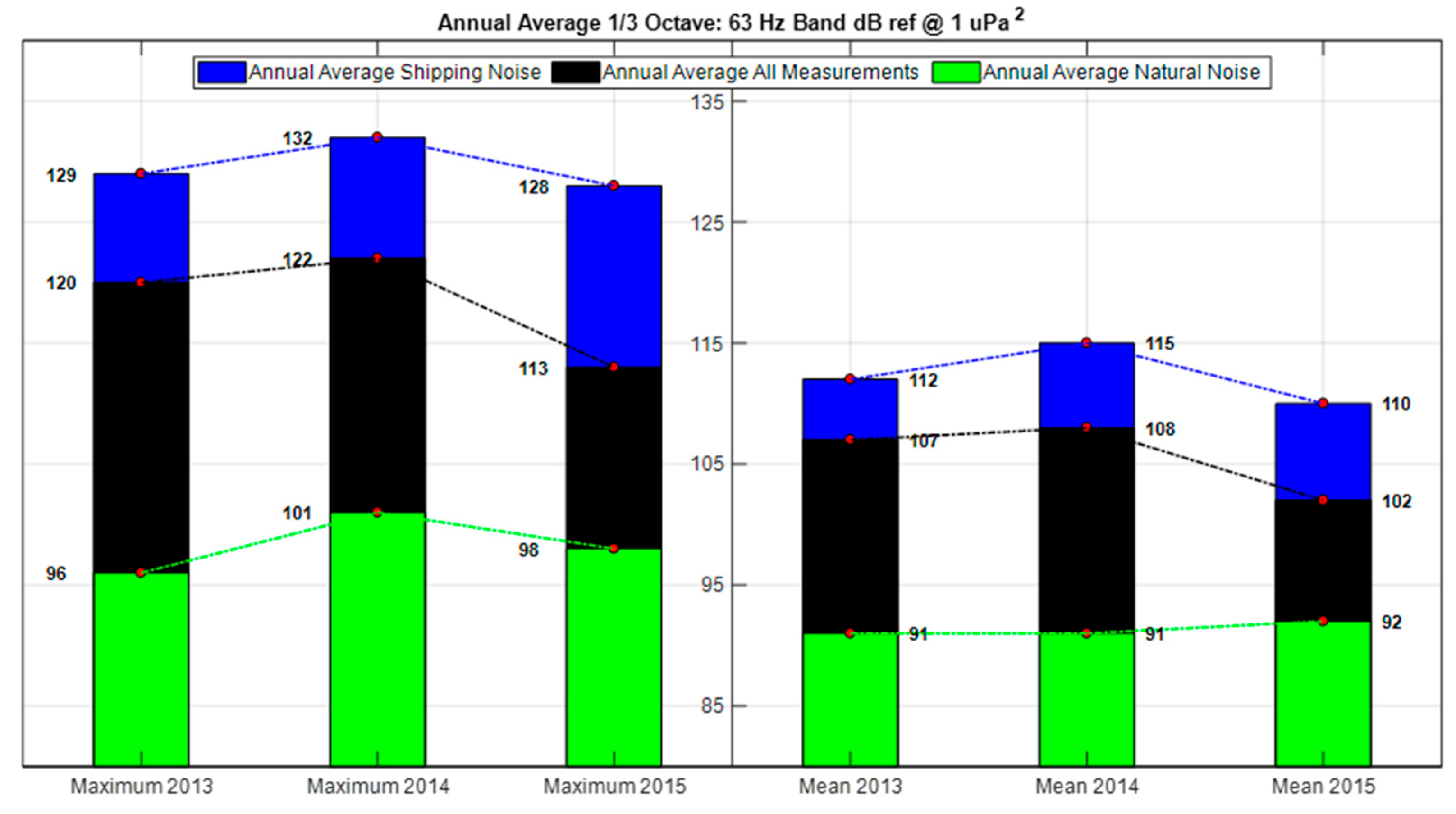
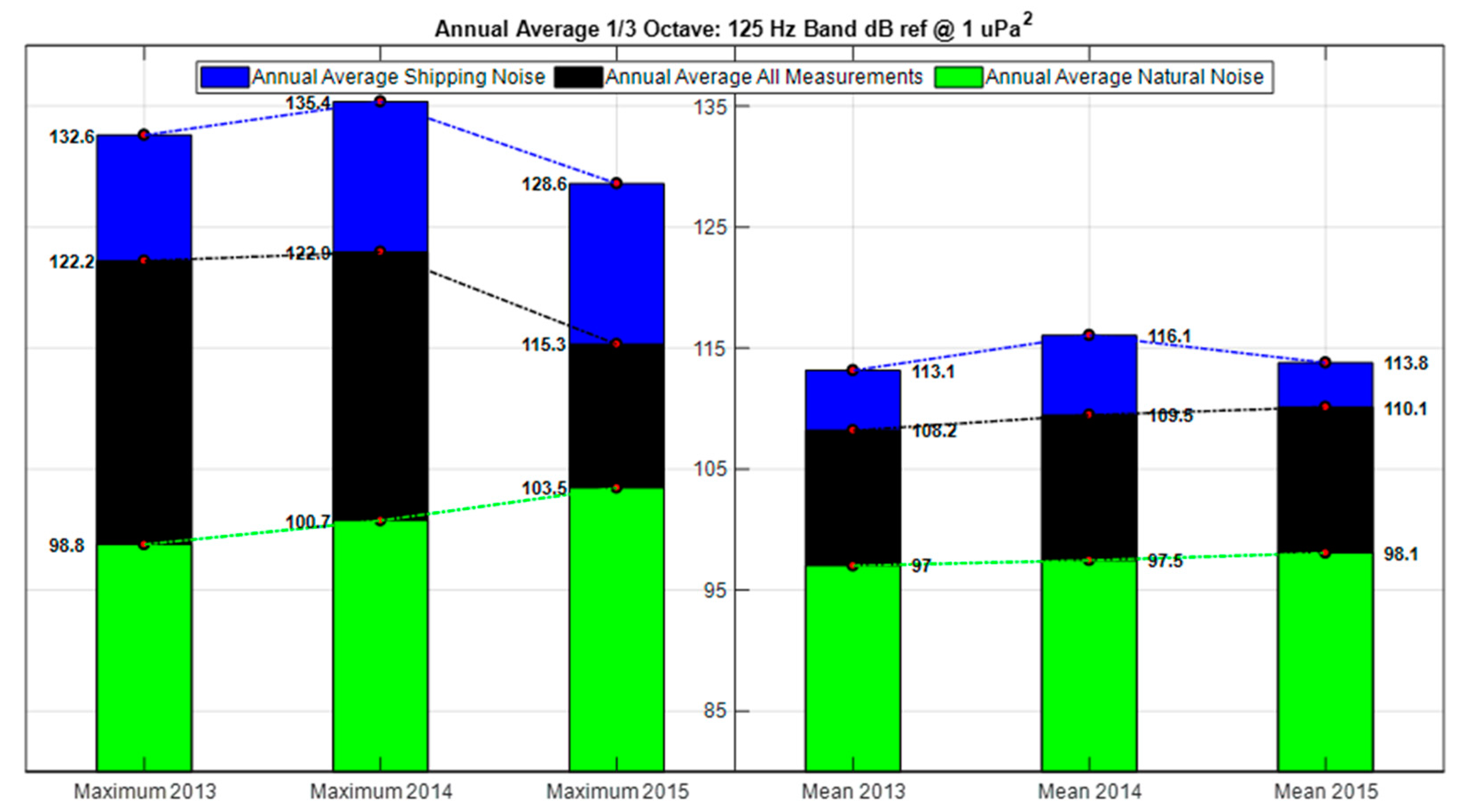
| Measurement Type | 63 Hz | 125 Hz | 63 Hz | 125 Hz | ||||
| Mean | SD | Mean | SD | Mean | SD | Mean | SD | |
| All | 106 | 3 | 109 | 3 | 119 | 5 | 120 | 5 |
| Shipping Noise | 113 | 4 | 115 | 3 | 130 | 4 | 133 | 5 |
| Natural Noise | 91 | 2 | 98 | 1 | 99 | 5 | 101 | 3 |
| Average in dB of the SPL Reference at 1 µPa2 | |||
|---|---|---|---|
| Statistical Indicator | Type of Measurement | ||
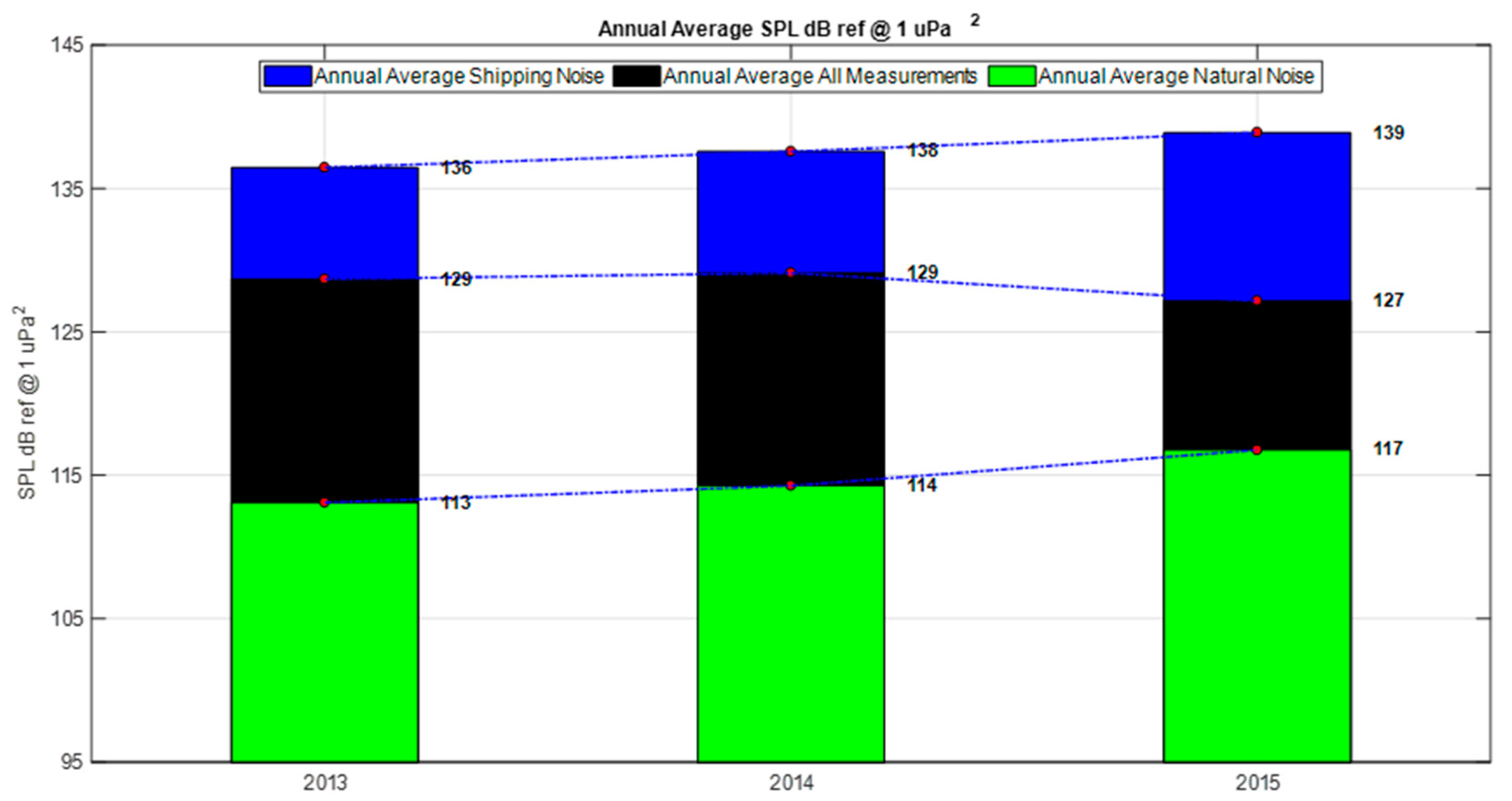
| All | Shipping Noise | Natural Noise | |
| Mean | 128 | 138 | 115 |
| Standard Deviation | 13 | 11 | 3 |
Publisher’s Note: MDPI stays neutral with regard to jurisdictional claims in published maps and institutional affiliations. |
© 2022 by the authors. Licensee MDPI, Basel, Switzerland. This article is an open access article distributed under the terms and conditions of the Creative Commons Attribution (CC BY) license (https://creativecommons.org/licenses/by/4.0/).
Share and Cite
Rodrigo, F.J.; Ramis, J.; Carbajo, J.; Poveda, P. Underwater Anthropogenic Noise Pollution Assessment in Shallow Waters on the South-Eastern Coast of Spain. J. Mar. Sci. Eng. 2022, 10, 1311. https://doi.org/10.3390/jmse10091311
Rodrigo FJ, Ramis J, Carbajo J, Poveda P. Underwater Anthropogenic Noise Pollution Assessment in Shallow Waters on the South-Eastern Coast of Spain. Journal of Marine Science and Engineering. 2022; 10(9):1311. https://doi.org/10.3390/jmse10091311
Chicago/Turabian StyleRodrigo, Francisco Javier, Jaime Ramis, Jesus Carbajo, and Pedro Poveda. 2022. "Underwater Anthropogenic Noise Pollution Assessment in Shallow Waters on the South-Eastern Coast of Spain" Journal of Marine Science and Engineering 10, no. 9: 1311. https://doi.org/10.3390/jmse10091311
APA StyleRodrigo, F. J., Ramis, J., Carbajo, J., & Poveda, P. (2022). Underwater Anthropogenic Noise Pollution Assessment in Shallow Waters on the South-Eastern Coast of Spain. Journal of Marine Science and Engineering, 10(9), 1311. https://doi.org/10.3390/jmse10091311