Article

CFD Investigation on Secondary Flow Characteristics in Double-Curved Subsea Pipelines with Different Spatial Structures

1
Marine Engineering College, Dalian Maritime University, Dalian 116026, China
2
National Center for International Research of Subsea Engineering Technology and Equipment, Dalian Maritime University, Dalian 116026, China
*
Author to whom correspondence should be addressed.
J. Mar. Sci. Eng. 2022, 10(9), 1264; https://doi.org/10.3390/jmse10091264
Submission received: 7 August 2022 / Revised: 2 September 2022 / Accepted: 2 September 2022 / Published: 7 September 2022
(This article belongs to the Special Issue Subsea Pipelines)

Abstract

:
Double-curved pipes are widely employed as essential components of subsea pipeline systems. Considering the layout flexibility and application diversity, there are various spatial structures for the double-curved combinations. However, few studies have compared the flow characteristics in different double-curved pipes. The dissipations of the corresponding downstream flow have not been thoroughly investigated, which are crucial for the measurement accuracy and flow assurance. In this paper, the turbulent flow in double-curved pipes with different spatial structures (i.e., Z-, U-, and spatial Z- type) was numerically studied by employing the ω-Reynolds stress model. The major purpose was to develop an in-depth knowledge on the secondary flow characteristics in different double-curved pipes and quantify the dissipations of the downstream flow. The effects of the spatial angle and interval distance of the two curves on the flow fields are taken into consideration, and the swirl intensity Si is introduced to evaluate the secondary flow dissipation. It is found that the secondary flows in the Z- and U-type structures are in opposite directions when the interval distance is short (3D), and the secondary flow in the spatial Z-type exhibits an oblique symmetric form. Only in the Z-type pipe with a short interval distance the secondary flow exhibits an exponential dissipation, and the fully developed flow is easier to achieve than the other cases. However, as the interval distance increases, the directions of the secondary flow in the U- and Z-type structures are the same, and the flow dissipations in all the structures return to the exponential types. The obtained dissipation rates for the secondary flow downstream of Z-, U-, and spatial Z-pipes with the 9D interval distance were 0.40, 0.25, and 0.20, respectively. The results are expected to guide the design of pipeline layouts and provide a reference for the arrangements of flowmeters in a complex subsea pipeline system.

1. Introduction

The subsea pipeline is the main part of the transportation of oil and gas products in the underwater production system and gained much attention [1,2]. To ensure the safety of energy transportation, many researchers have focused on corrosion [3], residual stress [4], buckling [5], and blocking [6] of the straight subsea pipelines. Moreover, the pipelines are not always straight in the underwater production system. To meet the flexibility of the spatial layout, they are designed as multicurved structures in which the flow fields are more complex than those in straight pipes.
In all curved structures, the 90° bends are the most basic components and widely employed in the subsea pipeline system. Different from the straight pipe, the curvatures of the bends cause the generation of secondary flow superimposed on the main flow. When passing through a 90° bend, the fluid with a high speed near the outer corner turns to the inner corner along the pipe wall, while the fluid with a low speed near the inner corner flows toward the outer corner as a result of the combined effect of the wall pressure gradient and centrifugal force. This fluid motion is firstly investigated in curved pipes by Dean and Chapman [7]. Therefore, the induced vortices are called as Dean vortices. In the decades since, the Dean motion in a curved pipe has been widely studied. The bifurcation of Dean vortices from a single pair to multipairs induced by the flow conditions and pipe geometries has been numerically discussed by Nandakumar and Masliyah [8], Yang et al. [9], and Yanase et al. [10]. Bovendeerd et al. [11] carried out an experiment to measure the secondary flow field in a bend at a Reynolds number of 700. Moreover, Sudo et al. [12,13] experimentally investigated the turbulent flow through the bent channels with square and circle sections. Jurga et al. [14] employed the Explicit Algebraic Reynolds Stress Model (EARSM) to investigate the turbulent flow in a bent pipe. Li et al. [15] adopted the computational fluid dynamics with discrete element method (CFD-DEM) to simulate the solid and liquid phase flow in a bent pipe and evaluated the degree of wall wear. Ning et al. [16] also used the CFD-DEM to study the solid–liquid flow through the channels with different curvature ratios. In recent years, the swirl-switching of the turbulent flow in a bent pipe has attracted increasing interest since this unsteady flow motion may cause fatigue damage to the pipelines. Hellström et al. [17] obtained that the two characteristic Strouhal numbers of the swirl-switching are 0.16 and 0.33 through a proper orthogonal decomposition (POD) method, which are in good agreement with those of Rütten et al. [18] and Kalpakli et al. [19]. Hufnagel et al. [20] conducted a direct numerical simulation (DNS) on the bent flow and concluded that the switching phenomenon is intrinsic to the bend geometry and independent of the upstream flow conditions. In addition, the complex flow physics in some other types of bending structures such as T-, plugged T-, and Y- junctions have been investigated. Sakowitz et al. [21] employed a large eddy simulation (LES) to investigate the turbulent flow mechanisms in a T-type junction. Ong et al. [22] and Han et al. [23,24] numerically investigated the laminar flow characteristics in the plugged T-junctions and reported the effect of structural parameters of the structures. Hu et al. [25] conducted a numerical and experimental study on the motion of particles in the Y-type bend and revealed that the particle transport is strongly affected by the secondary flow.
Since the pipeline system consists of straight, curved, and multicurved pipes, many researchers conducted studies on the flow in some kinds of bend combinations. Fiedler [26] conducted an experiment on the flow in double-curved pipes where the second bend is perpendicular to the first one and explained the asymmetries of the velocity profiles in the second bend. Mazhar et al. [27] carried out an experiment on the turbulent flow in S-shape 90° bends and found the higher turbulence kinetic energy near the downstream bend. In terms of the U-type bend, Sudo et al. [28] conducted an experiment to measure the flow field in the 180° bend. Moreover, some recent efforts have focused on the flow behaviors in double- [29] and triple-curved [30] pipes when the Reynolds number exceeds 107; the researchers attributed the flow-accelerated corrosion to the unsteady motions of the secondary flows in the bends. In terms of the multicurved structures, Liu et al. [31] numerically studied the flow characteristics and mixing conditions along the M-type jumper tubes with plugged T-junctions. Kim and Srinil [32] numerically studied the slug flows in the subsea M-type jumpers and evaluated the deformation and stress of the pipe.
In terms of the flow in multicurved pipes, the researchers generally focused on the specific curved structures such as Z-, S-, and U-type bend combinations. However, the effects of different spatial structures of the double-curved pipes on the flow behaviors and secondary flow characteristics have not been thoroughly investigated. Moreover, the secondary flow dissipation at the downstream of the double-curved pipes with various spatial structures has not been taken into consideration so far. Mattingly and Yeh [33] pointed out that the elbow-produced secondary flow will influence the flowmeter measurement accuracy. Research based on the elbow-produced secondary flow characteristics will guide the location of the flowmeter in the subsea pipeline system. Hence, in the present study, the turbulent flow in double-curved pipes with different spatial structures (i.e., Z-, U-, and spatial Z- type) was numerically studied using the Reynolds stress model based on the ω-equation (ω-RSM) to consider the anisotropy of turbulence. In addition, the RSM based on the ω-equation can provide a more accurate near-wall treatment, which was proved by Di Piazza and Ciofalo [34] to predict the satisfactory flow field in a coiled tube. The effects of the spatial angle and interval distance on secondary flow fields were thoroughly analyzed. The development of the velocity distributions, generations of the Dean vortices, and the dissipation of the swirl intensity were discussed in detail. The present study was intended to reveal the turbulent flow behaviors in the double-curved subsea pipelines and clarify the influence of spatial structures on secondary flow fields. The results are expected to guide the design of the subsea pipelines and provide a reference for the location of flowmeters.

2. Methodology

2.1. Governing Equations

In this study, the steady Reynolds–average Navier–Stokes (RANS) equations were solved, which can be described as
U i / x i = 0
U i U j / x j = 1 ρ p / x i + x j v U i x j u i u j ¯
where x i and x j (i, j = 1, 2, and 3) represent the three directions of the coordinate system, respectively;   U i and U j represent the corresponding time average velocity component; p represents the time average pressure; and ρ and v represent the density and kinematic viscosity of the fluid, respectively. u i u j ¯ is the Reynolds stress tensor, which is the time average value of the product of the fluctuations of the velocity component. The ω-Reynolds stress model (ω-RSM) is employed to solve the RANS equations, which avoids using the Boussinesq assumption employed in the eddy-viscosity model. It has been reported that the RSM is expected to capture more exact flow details when the secondary flows are induced by the curvatures [35]. The RSM directly resolves the transport equations of the Reynolds stress, which can be described as (ignoring the buoyancy)
t ρ u i u j ¯ + x k ρ u k u i u j ¯ = x k ρ u i u j u k ¯ + p δ k j u i + δ i k u j ¯ + p u i x j + u j x i 2 μ u i ¯ x k u j ¯ x k + x k μ x k u i u j ¯ ρ u i u k ¯ u j x k + u j u k ¯ u i x k
where the right-hand side of the equation includes the terms of turbulent diffusion, pressure strain correlation, dissipation, molecular diffusion, and stress production, respectively.
The ω-equation is defined as
ρ ω t + U k ρ ω x k = α ρ ω k P k β ρ ω 2 + x k μ + μ t σ ω ω x k
where the coefficients σ ω = 2, α = 5/9 β   = 0.075, μ t = ρ k / ω , and P k is the production rate of turbulence.
The turbulent diffusion term D T , i j , pressure strain correlation term ϕ i j , and dissipative term ε i j should be modelled to close the equations. The model equations (ω-based) are as follows:
D T , i j = x k ρ k ω σ k u i u j ¯ x k
ϕ i j = C 1 ρ β ω u i u j ¯ 2 3 δ i j k a ^ 0 ρ u i u k ¯ U j   x k u j u k ¯ U i   x k 2 3 δ i j p β ^ 0 ρ u i u k ¯ U k   x j ρ u j u k ¯ U k   x i 2 3 δ i j p γ ^ 0 ρ k S i j 1 3 S k k δ i j
ε i j = 2 3 δ i j ρ β k ω
where the coefficients are β = 0.09 ,   a ^ 0 = 8 + C 11 ,   β ^ 0 = 8 C 2 11 ,     γ ^ 0 = 60 C 4 55 ,   C = 0.52 ,   and   C 1 = 1.8 .
ANSYS CFX is employed to solve the RANS equations by an element-based finite-volume method. The total-variation-diminishing (TVD) scheme is employed for spatial discretization, which is of second-order accuracy. Since the ω-RSM does not use wall functions, the near-wall grids were densified in this study. The details of the corresponding meshing strategy will be discussed in Section 2.3.

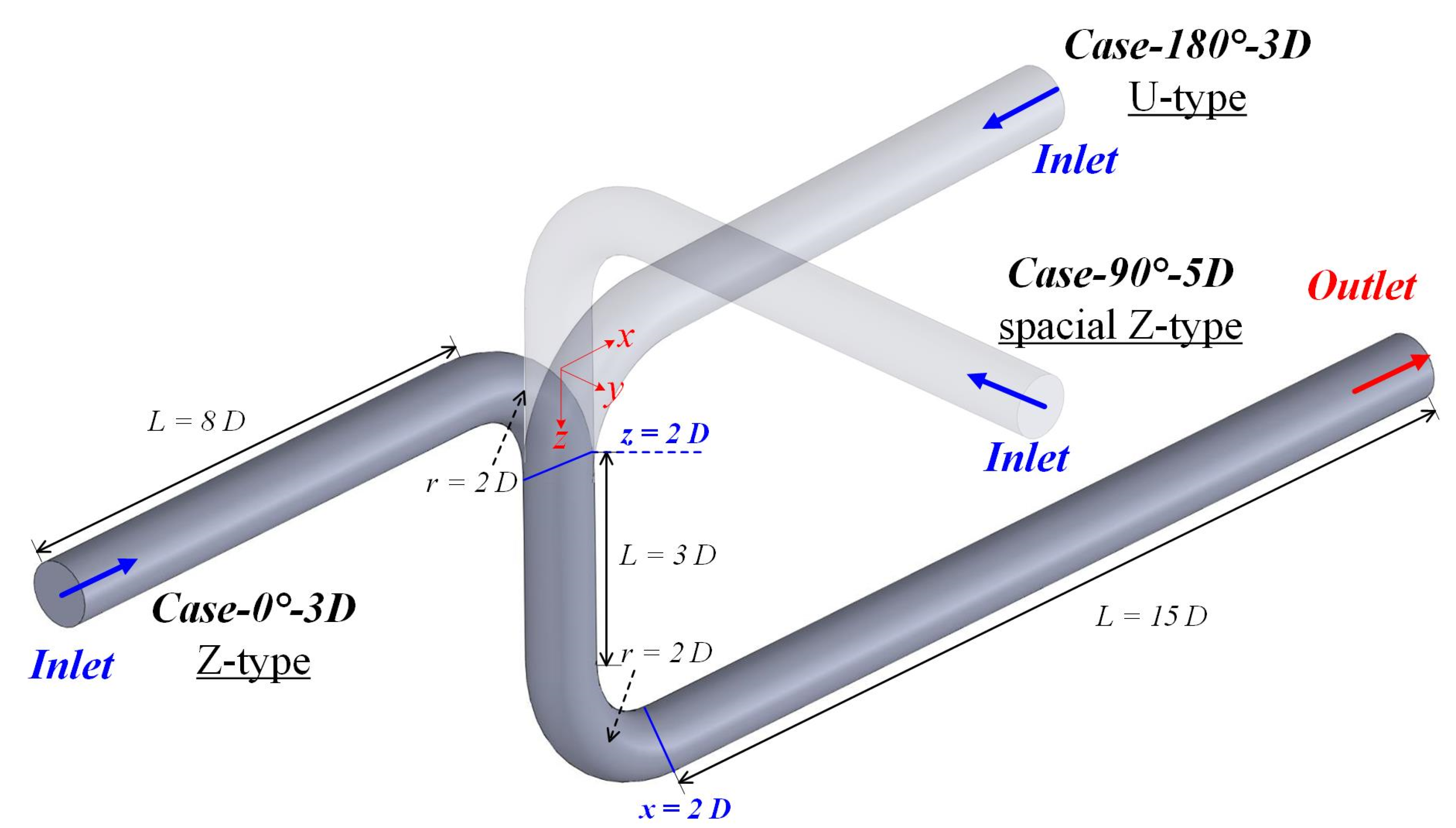
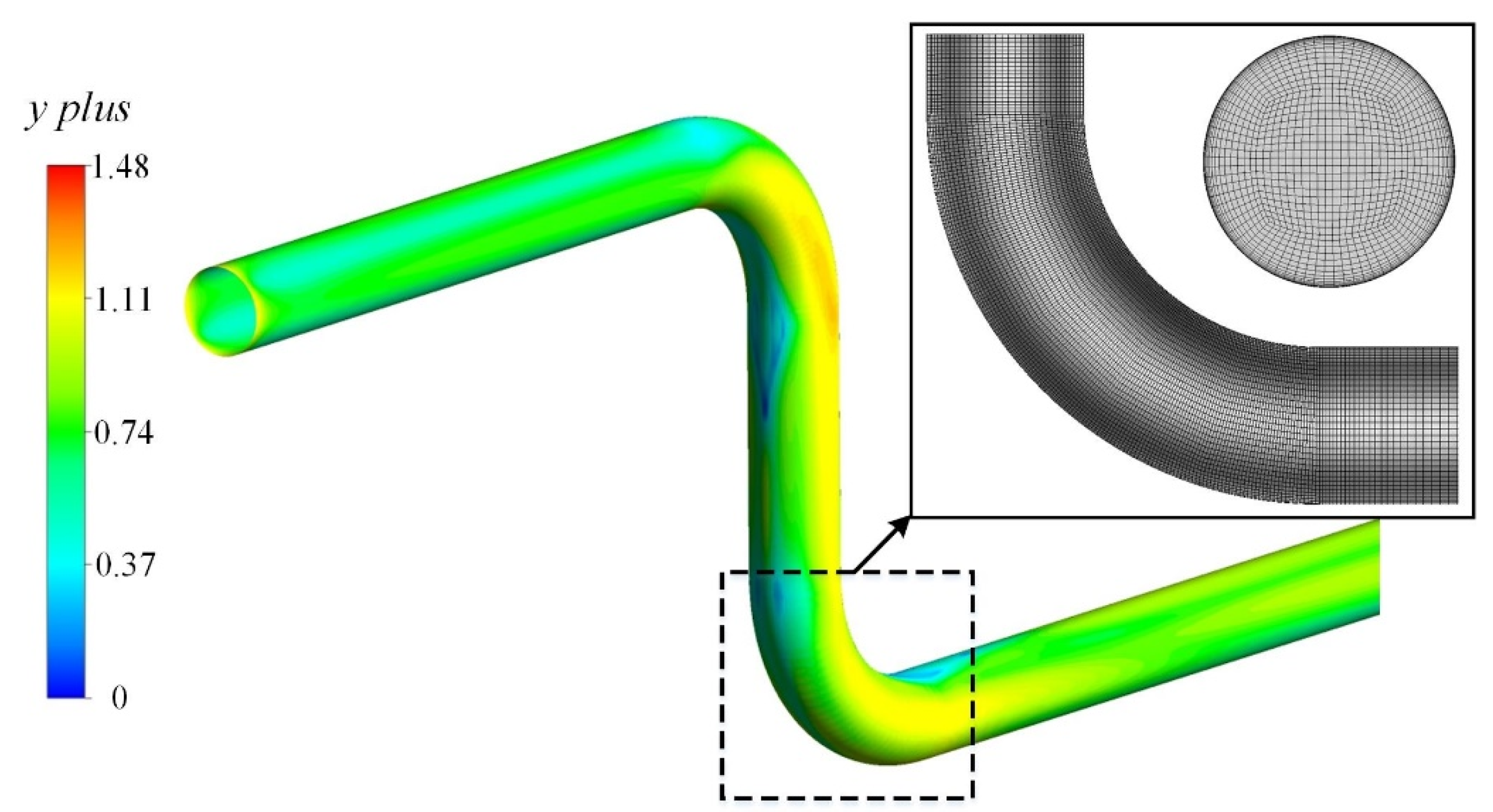
2.2. Computational Models

The calculation domains of the present study are displayed in Figure 1. The spatial angles between the upstream and downstream bends in three domains are 0°, 90°, and 180°, which represent the Z-, spatial Z-, and U-type pipes, respectively. The pipe diameter is defined as D = 1 m. The upstream length is 8D, and the downstream length is 15D. The curvature radius of the bend is 2D, and the interval distances between the two bends varied from 3D to 9D. For simplified description, different geometries analyzed in this paper are named with the double-bend angle and interval distance. As an example, the double-curved pipe with a spatial angle of 0° (Z-type) and an interval distance of 3D (i.e., the entity in Figure 1) is named as Case-0°-3D.
The zero normal gradient is specified for the inlet pressure condition, and the inlet velocity condition employs a modified power law profile from Salama [36]:
U = U b u l k β 1 , 1 + n 1 r R 2 1 n
where β is the Euler integral of the first kind, n = 0.77ln (Re)-3.47, U b u l k   = 10 m/s is the inlet bulk velocity, r is the distance from the location to the center of the cross section, and R is the pipe radius.
The reference pressure is zero at the outlet, where the velocity is defined as the zero normal gradient. The zero normal gradient is specified for the wall surface, and the flow velocity employs a nonslip boundary condition.

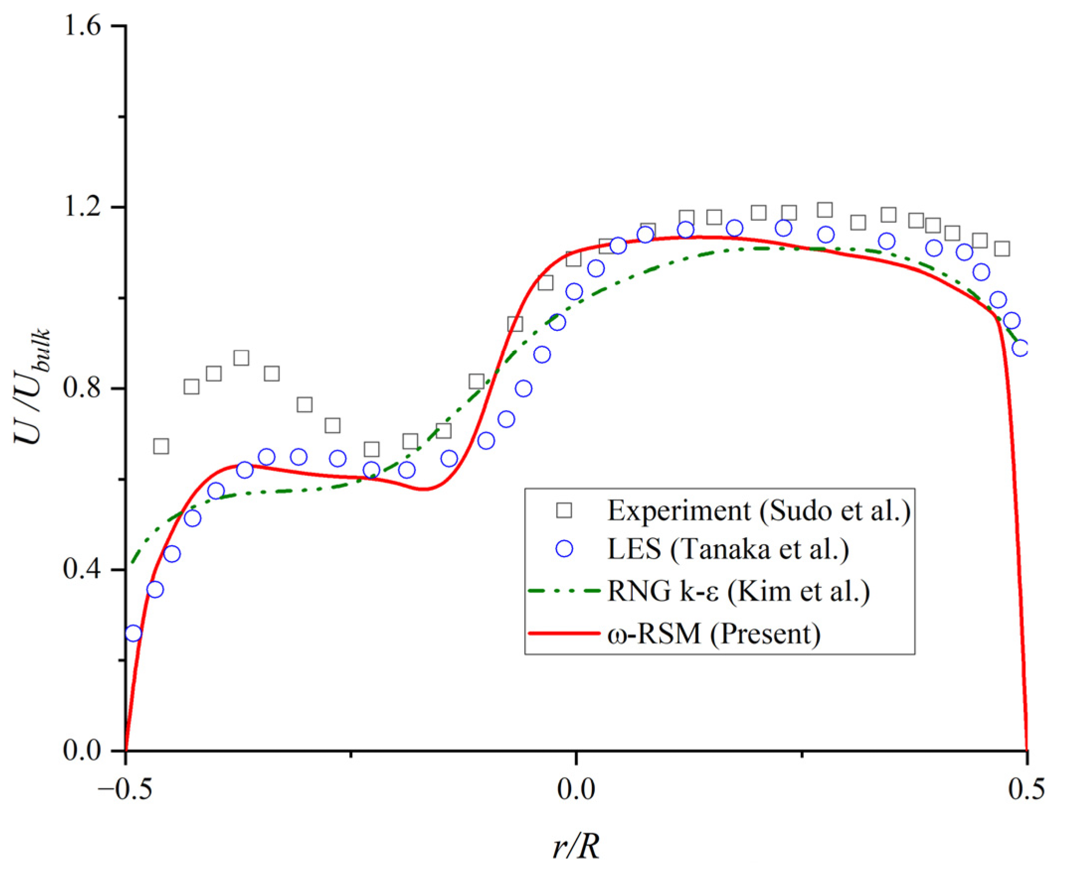
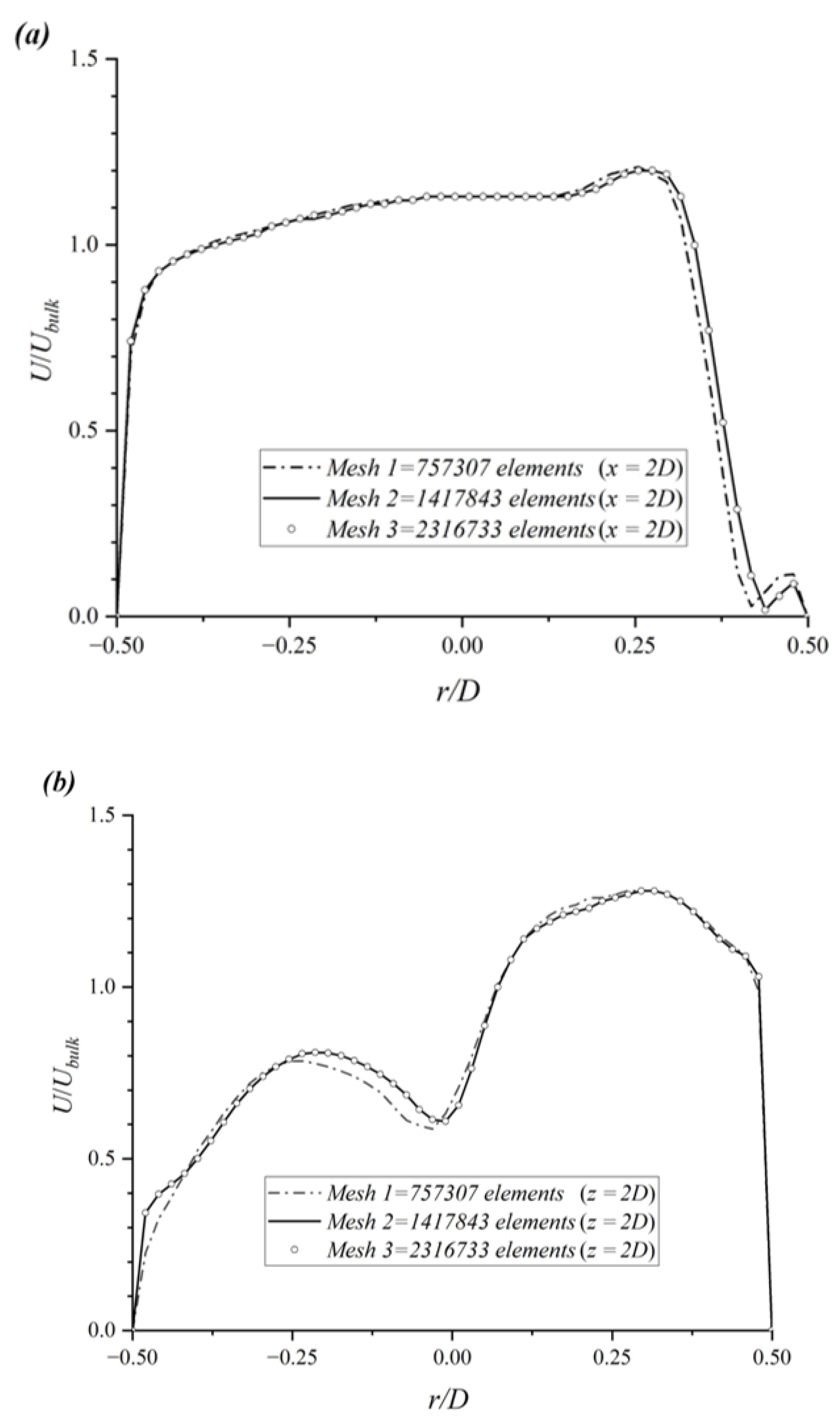
2.3. Verification and Validation Study

In this section, the mesh convergence study was firstly carried out, and then the numerical method employed in this study was validated by comparing with the published results. The verification study was conducted to obtain a suitable mesh for the current study. The flow in the Z-type double-curved pipe with the interval distance of 3D (i.e., the entity in Figure 1) at a Reynolds number of 10,000 is provided as an example. Three sets of structured grids for the computational domain have been generated, and the distributions of the velocity at the outlets of the upstream and downstream bends (i.e., z = 2D and x = 2D) are shown in Figure 2. Obvious divergences can be observed between the results in mesh 1 with 757,307 elements and mesh 2 with 1,417,843 elements, while good consistency can be found between mesh 2 with 1,417,843 elements and mesh 3 with 2,316,733 elements. It is found that the mean deviations between mesh 1 and mesh 2 at the outlet of the first and second bends are 2.46% and 2.27%, respectively. However, the mean deviations between mesh 2 and mesh 3 are 0.11% and 0.23%, respectively. In addition, the max deviations between mesh 1 and mesh 2 at the outlet of the first and second bends are 11.59% and 17.34%, while the corresponding deviations between mesh 2 and mesh 3 are only 0.498% and 0.723%, respectively. Hence, mesh 2 (1,417,843 elements), which can provide sufficient numerical accuracy, was employed in the present study. The contour of y + and details of mesh 2 are shown in Figure 3. The average y + value is calculated as 0.798 ( y + = Δ y u / v , where u is the friction velocity, and Δ y is the distance from the first grid to the wall).
Then, a validation study was carried out to confirm the reliability of the numerical method. The turbulent flow through a 90° bend with the curvature ratio of 2 at a Reynolds number of 60,000 has been widely investigated with experiments [12] and numerical simulations [37,38]. For validation purposes, the numerical study was carried out on the same bend structure under the same flow condition using the obtained meshing strategy and ω-RSM. Then, the outlet velocity distribution of the bend obtained by the current simulation was compared with the published results to validate the numerical method in the present study. Figure 4 shows the velocity distributions at the elbow outlet obtained by the experiment and different numerical methods. Except for the region near the inner-side wall, the numerical results are close to the experiment data. However, the velocity distribution obtained with the ω-RSM is closer to the results of LES prediction [37] than that of the RNG k-ε model [38]. It indicates that the ω-RSM can obtain a more accurate result than the RNG k-ε model in predicting the curved flow, which is consistent with the conclusion of Di Piazza and Ciofalo [34]. Furthermore, the ω-RSM with a lower computational cost can provide a similar near-wall prediction as the LES method. Therefore, comprehensively considering the advantages on the numerical accuracy and computational cost, the ω-RSM was validated and employed in the present study. It also shares the same view as Wallin and Johansson [35] and Pruvost et al. [39].

2.4. Definition of Swirl Intensity

In order to quantitatively evaluate the developments of the secondary flow and swirling strength, the swirl intensity S i is employed in the following studies, which is introduced by Sudo et al. [12]. The swirl intensity S i can be described as
S i = U U n ^ n ^ 2 d A / U b u l k 2 d A
where n ^ represents the unit vector parallel to the flow direction, and U represents the vector of the flow velocity.

3. Results and Discussions

Since the numerical method has been validated in Section 2.3 with the studies of Sudo et al. [12], Tanaka et al. [37], and Kim et al. [38], the ω-RSM and verified meshing strategy are employed in the following sections to investigate the turbulent flow in the double-curved pipes with different spatial structures at a Reynolds number of 10,000. The effects of the spatial angle and interval distance between two bends have been discussed.

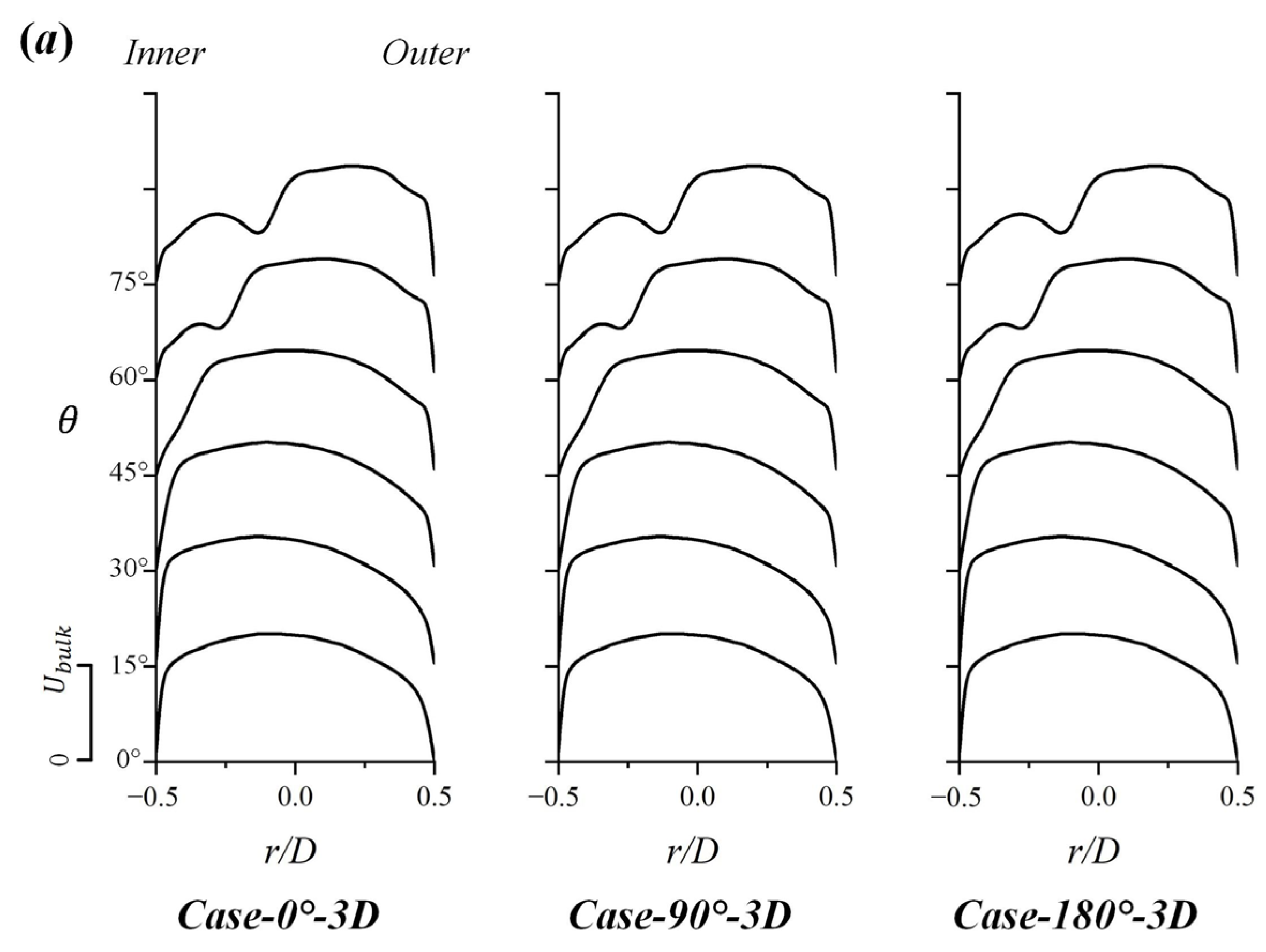
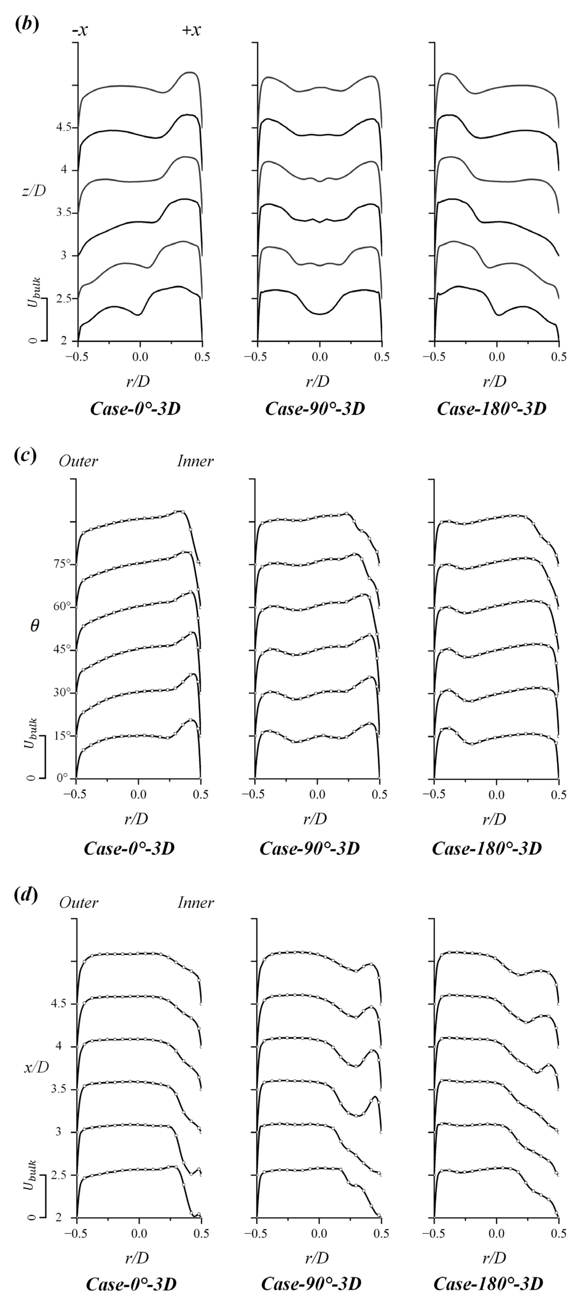
3.1. Effect of Spatial Angle

To provide an intuitive understanding on how the upstream bends at different spatial angles affect the downstream flow fields, the cross-sectional velocity fields at the outlets of the first bends, the global streamlines, and the velocity vectors downstream of the first bends in Case-0°-3D, Case-90°-3D, and Case-180°-3D are shown in Figure 5. The vector fields are displayed in the symmetric plane of the second bend (i.e., the x-z plane) in all the structures to compare the effect of the spatial angle on the flow fields in the downstream bends. For the first bend, the flow conditions in different structures are the same as shown in Figure 5a. However, the vector field in the x-z plane changes with the variation of the spatial angle from 0° to 180°, leading to different inlet conditions of the downstream bends.
In addition, the velocity vectors downstream of the first bends show significant differences with the spatial angles between two bends varying from 0° to 180°. A high-velocity region appears near the +x direction in the intermediate pipe of Case-0°-3D, while the region appears near the −x direction in Case-180°-3D. In addition, the velocity vectors in the intermediate pipe of Case-90°-3D display an asymmetrical distribution. The high-velocity region appears near the pipe wall, while the low-velocity region appears at the center of the cross-section. At the downstream of the second bend, the flow becomes quite uniform in Case-0°-3D. However, as the spatial angle increases, the velocity near the outer corner of the downstream bend increases. The result indicates that it is easier for the flow to achieve full development when the spatial angle is 0° as compared with the other cases. Since the low-velocity areas near the inner corner of the second bend (black-dotted rectangles) are hard to be observed in the whole vector fields, the velocity vectors in these areas are magnified alongside. It can be found that the velocity gradient in Case-0°-3D is higher than the other cases. In addition, the flow separation can be clearly observed in Case-0°-3D, while it greatly reduces in Case-180°-3D.
Figure 6 illustrates the developments of the flow distribution in the (a) first bends, (b) intermediate pipe between two bends, (c) second bends, and (d) downstream of second bends in Case-0°-3D, Case-90°-3D, and Case-180°-3D. The locations of the selected profiles are shown in Figure 6e. It is found that the velocity distributions in the first bends are very similar to each other, which is physically sound. In the intermediate pipe, the velocity profiles of Case-90°-3D display symmetric bimodal distributions since the upstream bend is perpendicular to the x-z plane. The velocity profiles in Case-0°-3D and Case-90°-3D show the contrary unimodal distributions due to the opposite directions of the upstream bends. It is worth noting that the divergences in Figure 6b are due to the different spatial angles and same selected coordinates. When the fluid enters the second bend, as shown in Figure 6c, the symmetries of velocity distributions are broken, and the velocity near the inner corner increases in Case-90°-3D. In addition, the peak velocity gradually moves toward the center of the pipe as the bending angle θ increases. A similar phenomenon can be observed in Case-0°-3D; however, the velocity near the inner corner is lower than that in Case-90°-3D. In Case-180°-3D, the velocity peaks appear in both inner and outer corners. More specifically, the outer-corner peak is due to the upstream flow distribution, and the inner-corner peak is induced by the bend curvature. At the outlet of the second bend, velocity fluctuations are found near the inner corner at x/D = 2 and 2.5 in Case-0°-3D, implying the flow separation area. However, the separation area can hardly be seen in Case-90°-3D and Case-180°-3D, which is consistent with the qualitative analysis in Figure 5. As the downstream distance increases, the flow in Case-0°-3D more rapidly restores uniformity than the other cases. High-velocity gradients can still be observed near the inner corner at x/D = 4.5 in Case-0°-3D, Case-90°-3D, and Case-180°-3D. It is concluded that, for structures with a short interval distance, the flow downstream the first bend is not fully developed before the second bend. Therefore, the downstream flow is deeply influenced by the upstream bend with different spatial structures, and the flow fields downstream of the second bend are more complex than those of the first bend.
Furthermore, the effect of different spatial structures on the secondary flow characteristics downstream of the double-curved pipes was investigated. Figure 7, Figure 8 and Figure 9 display the streamlines on the selected positions (i.e., x/D = 2, 2.5, 3, 3.5, 4, 4.5, and 5) at the downstream of Case-0°-3D, Case-180°-3D, and Case-90°-3D, respectively. The streamlines are colored with dimensionless tangential velocity U t x / U b u l k = U z 2 + U y 2 / U b u l k , where U z and U y represent the velocity components in the z and y directions, respectively. As shown by Case-0°-3D in Figure 7, the fluid near the inner corner rushes to the outer corner at a high tangential velocity owing to the influence of centrifugal force at x = 2D. Then, the outer-corner fluid turns back through the center line and finally forms a pair of vortices, which is called the Base vortices defined by Bhunia and Chen [40]. In addition, an extra pair of vortices can be observed near the inner corner and finally disappears in 1.5D downstream (i.e., x = 3.5D). This pair of vortices characterizes the same motion as the inner-corner Dean vortex described by Bhunia and Chen [40] and Dutta and Nandi [41]. However, a branching generates near the inner corner and leads to another pair of vortices near the inner-corner Dean vortex at x = 2.5D, which has not been reported in the single bend so far. Hence, this branching is considered to be caused by the upstream bend.
Figure 8 displays the secondary flow fields in Case-180°-3D. The secondary flow motion in Case-180°-3D is contrary to that in Case-0°-3D. The fluid near the inner corner rushes to the outer corner through the center line, while the outer-corner fluid turns to the inner corner along the pipe wall on both sides. It is found that there is no vortex generation at x = 2D. However, as the downstream distance increases, two pairs of vortices first generate near the inner corner at x = 2.5D. Subsequently, the vortices near the inner corner split, and an extra pair of vortices generates near the pipe center at x = 3D. As the downstream distance increases from 1.5D (i.e., x = 3.5D) to 3D (i.e., x = 5D), the split vortices merge by degrees and eventually form one pair of large vortices at x = 5D. In terms of the velocity distribution, the high tangential velocity areas appear near the inner corner in Case-180°-3D, whereas they appear near the pipe center in Case-0°-3D. Then, as shown by the streamlines in Figure 9, the inclined secondary flow motion in Case-90°-3D can be found, which is induced by the vertical upstream bend. A high tangential velocity area occurs at one side of the inner corner and forms a main vortex. As the downstream distance increases, the other three vortices generate and eventually form a tilt symmetric four-vortex structure. It is found that the directions of the adjacent vortices are opposite, and the main vortex near the inner corner occupies the most tangential momentum. According to the above discussion, it is revealed that changing the spatial angle between the upstream and downstream bends in the double-curved pipe will redistribute the velocity field, reverse the flow direction, and break the central symmetry of the secondary flow at the downstream.
Subsequently, to quantify the intensities of the secondary flow in Case-0°-3D, Case-90°-3D, and Case-180°-3D, the swirl intensity S i introduced in Section 2.4 is employed. Figure 10 shows the developments of the swirl strengths along Case-0°-3D, Case-90°-3D, and Case-180°-3D. It is worth noting that the swirl strengths are selected every 0.5D length in the straight pipe sections and every 15° from 0° to 90° in the bends. The shaded sections represent the upstream and downstream bends. It is found that S i has slightly increased before the first bend and then increases by a wide margin in the first bend. Subsequently, S i shows a sharp decline at the intermediate pipe after outflowing from the first bend. The developments of S i in Case-0°-3D, Case-90°-3D, and Case-180°-3D are quite similar in the above process. However, significant differences can be observed inside and downstream of the second bends. S i increases in the second bend of Case-0°-3D and Case-90°-3D, whereas it decreases in the second bend of Case-180°-3D. The phenomenon indicates that the effect of the downstream bend on S i is strongly related to the spatial structure of the bend. At the outlet sections of the double-curved pipes, the dissipation rate of S i in Case-90°-3D is larger than that in Case-0°-3D, although their initial values are almost the same. In addition, the dissipation rate of S i in Case-180°-3D is the highest.
In order to further analyze the dissipation trends of the swirl intensities, the values of Case-0°-3D, Case-90°-3D, and Case-180°-3D obtained with Equation (9) are displayed in Figure 11 with a logarithmic ordinate and compared with the result of a traditional single bend reported by Kim et al. [38]. The dissipation of swirl intensity S i in the single bend is an exponentially decreasing function given as follows [38]:
  S i = S i 0 e β s L s / D  
where S i 0 represents the swirl intensity at the bend outlet, β s represents the dissipation rate, L s represents the downstream distance from the outlet of the second bend, and D represents the diameter of the pipe.
The value of β s is reported as 0.21, and the dissipation is weakly related to the Reynolds number [38,42]. However, as shown in Figure 11, the dissipations of swirl intensities are not exactly exponential in double-curved pipes. Only the swirl intensity in Case-0°-3D can be considered to express as exponential dissipation (exclude the initial value), and the β s is fitted as 0.30. In addition, it is found that the swirl intensity of Case-90°-3D is stronger than that of Case-180°-3D when L s / D 4 and becomes weaker when L s / D > 4 . Hence, the different spatial structures of the double-curved pipes can greatly influence the secondary-flow strength and break the exponential dissipation at the downstream of the pipes. Only the downstream flow in Case-0°-3D approximately conforms the exponential dissipation.

3.2. Effect of Interval Distance

In this section, the interval distance is increased to 9D, and the corresponding velocity profiles, secondary flow characteristics, and dissipations of the swirl intensity have been investigated and compared with the results in Case-3D. Figure 12 shows the comparisons of velocity profiles at the inlets and outlets of the downstream bends in (a) Case-0°-3D and Case-0°-9D; (b) Case-90°-3D and Case-90°-9D; and (c) Case-180°-3D and Case-180°-9D. As the interval distance increases, the velocity profiles at the inlets of the downstream bends become gentler, which is physically sound. The high-velocity areas near the outer corner become smaller, and the velocities decrease near the center lines in all configurations when the interval distances increase to 9D. The velocity profiles at the bend outlet in the double-curved pipe approach to the single-bend distributions when the interval distance increases. In addition, the separation area in Case-0°-3D disappears when the distance between the two bends increases to 9D. It implies that the flow before the second bend starts to be developed with the increase in the interval distance, resulting in a more stable flow condition near the inner corner of the second bend.
To further compare the secondary flow characteristics in the double-curved pipe with interval distances of 3D and 9D, the streamlines at the outlets of the downstream bends (i.e., x = 2D) in Case-0°-9D, Case-90°-9D, and Case-180°-9D are displayed in Figure 13 and compared with the streamlines of Case-3D in Figure 9. The downstream tangential velocity in Case-9D is higher than that in Case-3D, indicating that the too short interval distance (3D) will limit the tangential momentum exchange in the double-curved pipe. Moreover, the high-velocity area appears near the pipe center in Case-0°-3D and forms a pair of vortices, while the area is near the inner corner of the pipe in Case-0°-9D. A similar phenomenon can be observed in Case-180°-3D and Case-180°-9D. It has been mentioned that the secondary flow motions are greatly influenced by the spatial angle of the upstream bend when the interval distance is short (3D). However, when the interval distance increases to 9D, the fluid rushes to the outer corner from the center line and turns back from the pipe wall in all configurations, showing similar secondary flow motions. In addition, the vortex direction of the secondary flow in Case-0°-9D is opposite to that in Case-0°-3D. Hence, it can be concluded that increasing the interval distance of the two bends will weaken the effect of the upstream bend and lead to contrary secondary flow motions.
Figure 14 shows the dimensionless vortices iso-surfaces by the Q -criterion [43] in Case-0°-3D, Case-90°-3D, Case-180°-3D, Case-0°-9D, Case-90°-9D, and Case18-0°-9D to discuss the effect of the interval distance on the vortex structures in double-curved pipes. The Q -criterion can be defined as Q = Ω 2 S 2 / 2 , where Ω represents the rotation tensor, and S represents the strain tensor. The dimensionless value is Q = Q D 2 / U b u l k 2 = 0.5 , which is colored by the velocity. In addition, the criterion contours of the x-components Q x at x = 4D are printed alongside. It can be clearly observed that the pair of vortex cores moves toward the inner corner at the downstream of the pipe in Case-0° when the interval distance increases. In Case-90°, the vortices are inclined since the angle between the two bends are perpendicular. In terms of the vortices in Case-180°, additional sweeping structures generate when the interval distance increases. It is found that the distributions of downstream vortices are various in different structures when the interval distance is 3D. However, the vortices are close to the inner sides in all structures when the interval distance increases to 9D. In addition, as the interval distance increases, more vortices generate at the downstream of the pipes. The above phenomenon implies that a short interval distance limits the generation of the vortex at the downstream of the pipe. Increasing the interval distance will lead to similar vortex structures in the double-curved pipe.
Subsequently, a comparison of swirl intensities downstream of Cases-9D (i.e., Case-0°-9D, Case-90°-9D, and Case-180°-9D) and Cases-3D (i.e., Case-0°-3D, Case-90°-3D, and Case-180°-3D) is shown in Figure 15a. The initial values of S i in Cases-9D are higher than those in Cases-3D since the higher tangential velocity in Cases-9D enhances the strength of the downstream swirls (see Figure 9 and Figure 13). In 1D downstream, sharp decreases in swirl intensities occur in Cases-3D. However, the swirl intensities exhibit the exponential dissipations in Cases-9D. To reveal the dissipation rates of the swirl intensities in Cases-9D, Figure 15 (b) displays the dissipation of S i in a logarithmic coordinate. The dissipation rates β s for Case-0°-9D, Case-90°-9D, and Case-180°-9D (exclude the initial values) can be fitted as 0.40, 0.20, and 0.25, respectively, indicating the highest dissipation rate in Case-0°-9D. To sum up, the short interval distance (3D) will limit the swirl intensity downstream of the double-curved pipes, which coincides with the result from the analysis of vortex structures. With the increase in the interval distance, the flow before the second bend starts to be developed. As a result, the effect of the spatial angle is weakened, and the dissipation of the swirl intensity downstream the second bend gradually conforms to an exponential form, which is similar to a single-bend case.

4. Conclusions

In this paper, a numerical study was conducted on the turbulent flow in double-curved pipes with different spatial structures. The effects of the spatial angle and interval distance between the two bends on the secondary flow were thoroughly investigated with the vector fields, velocity distributions, vortex developments, and dissipations of swirl intensity. Major conclusions are listed as follows:
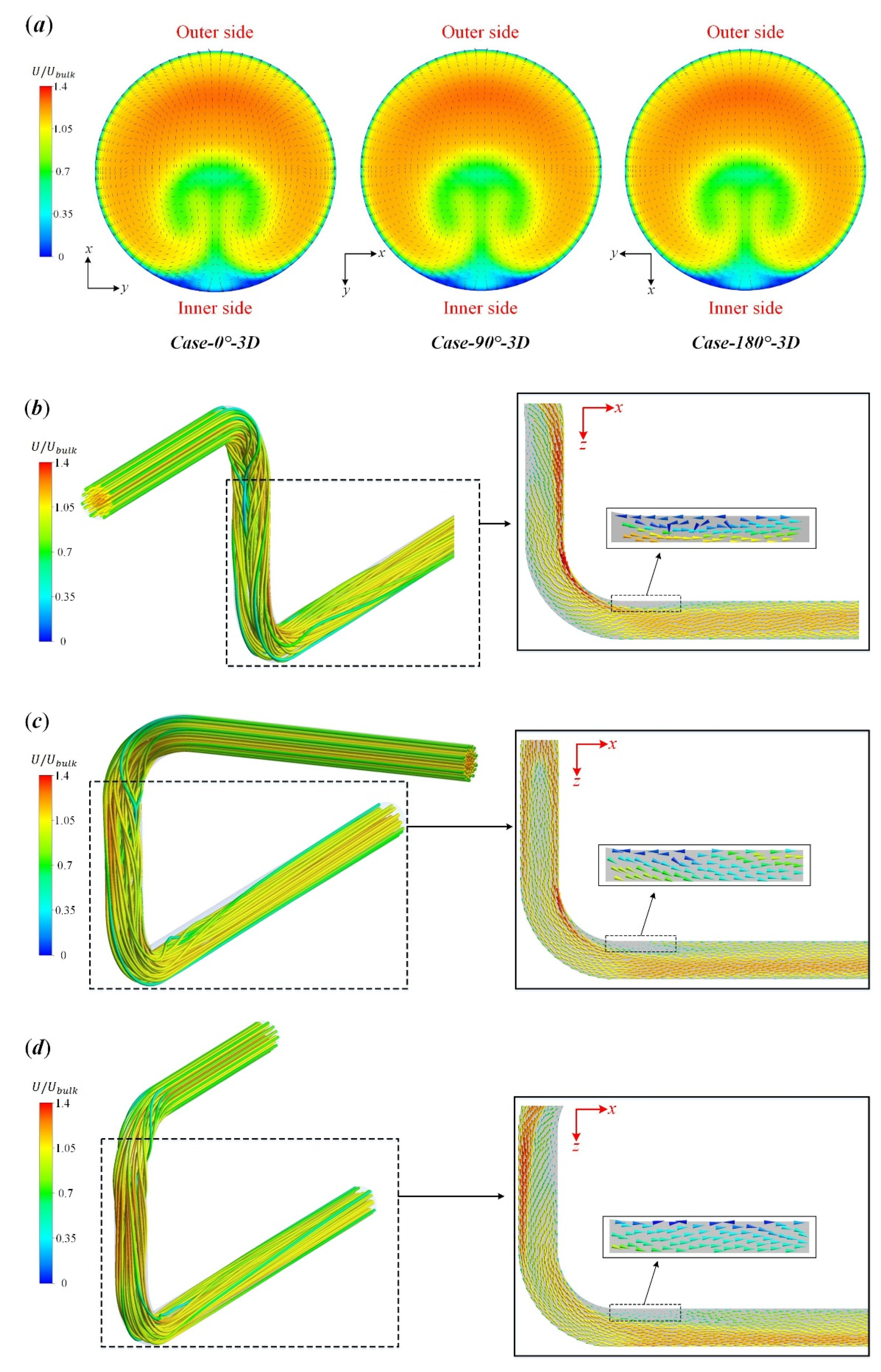
  • The directions of the secondary flows in the Z- and U-type pipes are opposite when the interval distance between the two bends is short (3D). In addition, the secondary flow in the spatial Z-type structure is biased by the upstream bend and exhibits an oblique symmetric type.
  • The vortex generations downstream of different double-curved pipes are limited when the interval distance is short. However, increasing the interval distance of the two bends will lead to similar secondary flow motions and vortex structures even if their spatial structures are different.
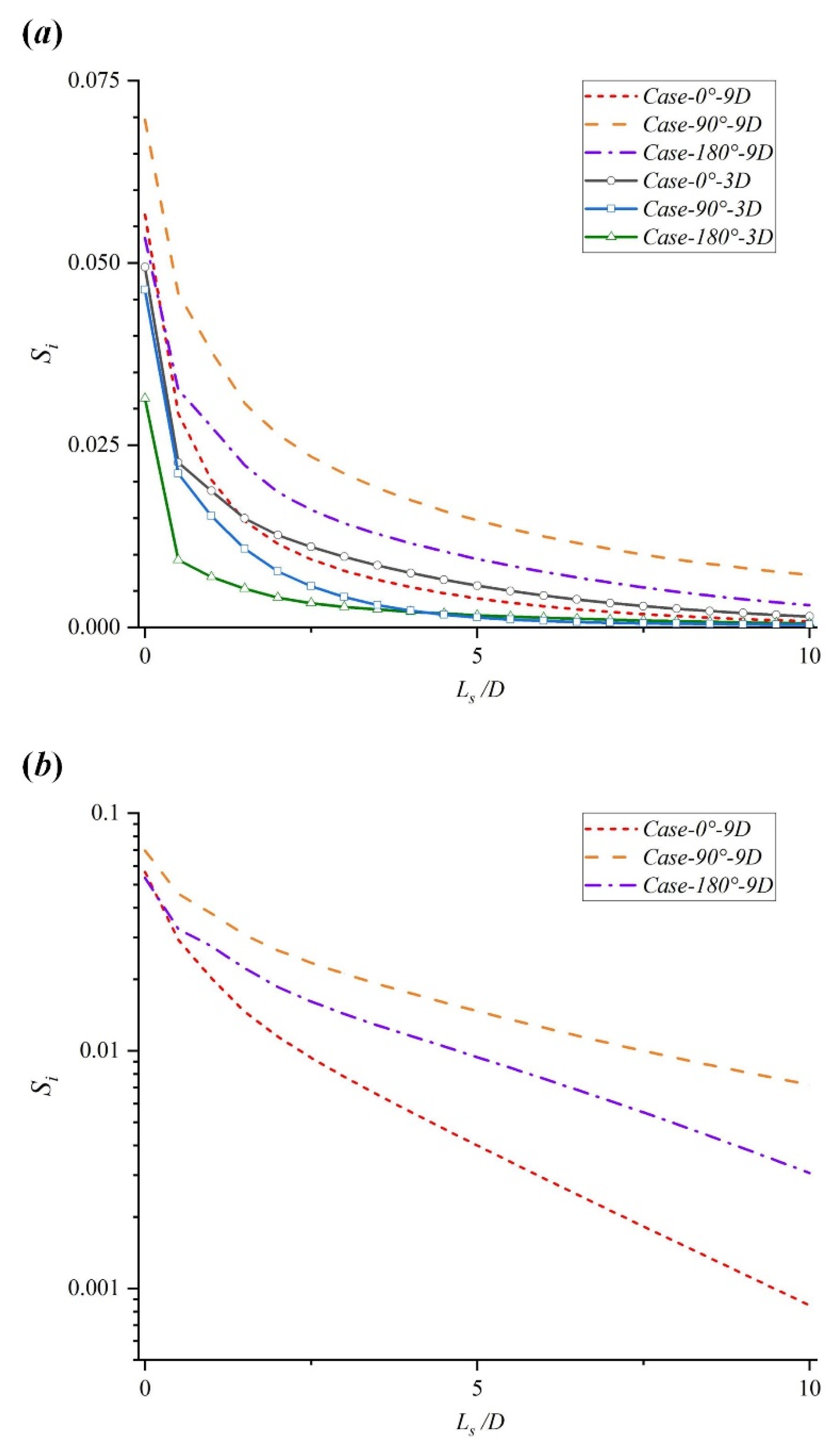
  • When the interval distance is short, only in the Z-type pipe, the downstream flow dissipates in an exponential form, and it is easier to achieve a fully developed flow than the other cases. However, the downstream flow recovers the exponential dissipations in all the structures when the interval distance increases to 9D. The corresponding dissipation rates of the downstream swirl intensities in the Z-, U-, and spatial Z-pipes are 0.40, 0.25, and 0.20, respectively.
The present study provided an in-depth knowledge on the secondary flow characteristics in double-curved subsea pipelines with different spatial structures. The results can provide guidance for the layout design of subsea pipelines and the arrangement of flowmeters. In terms of the pipeline design, a short interval distance between two bends will limit the swirl strength to obtain a more accurate flow measurement, and the U-type double-curved pipe inducing the weakest swirl is the most beneficial. In addition, increasing the interval distance between the two bends will weaken the effect of the spatial structure and strengthen the swirls. For the locations of flowmeters, it is not recommended to be arranged within 1D downstream the bend outlet to avoid the sharp variation of the swirl strength. For further research, the effect of the bend curvature and inlet flow condition should be taken into consideration.

Author Contributions

Conceptualization, F.H. and Z.W.; methodology, F.H. and Y.L.; software, Y.L.; validation, Y.L. and Q.L.; investigation, F.H., Y.L., Q.L. and Z.W.; writing—original draft preparation, F.H. and Y.L; writing—review and editing, F.H., W.L. and Z.W.; supervision, Z.W.; project administration, W.L.; funding acquisition, F.H. and Z.W. All authors have read and agreed to the published version of the manuscript.

Funding

This work was supported by the National Natural Science Foundation of China (No. 52006022), Liaoning Provincial Natural Science Foundation of China (No. 2022-MS-154), Dalian High-Level Talent Innovation Support Project (No. 2021RQ040), Scientific Research Funding Project of the Education Department of Liaoning Province (No. LJKZ0058), China Postdoctoral Science Foundation (No. 2020M670726), Fundamental Research Funds for the Central Universities (No. 3132022350), and 111 Project (No. B18009).

Data Availability Statement

Not applicable.

Conflicts of Interest

No potential conflict of interest was reported by the authors.

References

  1. Chen, B.-Q.; Videiro, P.M.; Guedes Soares, C. Opportunities and Challenges to Develop Digital Twins for Subsea Pipelines. J. Mar. Sci. Eng. 2022, 10, 739. [Google Scholar] [CrossRef]
  2. Chen, B.-Q.; Zhang, X.; Guedes Soares, C. The effect of general and localized corrosions on the collapse pressure of subsea pipelines. Ocean Eng. 2022, 247, 110719. [Google Scholar] [CrossRef]
  3. Yu, J.; Xu, W.; Yu, Y.; Fu, F.; Wang, H.; Xu, S.; Wu, S. CFRP Strengthening and Rehabilitation of Inner Corroded Steel Pipelines under External Pressure. J. Mar. Sci. Eng. 2022, 10, 589. [Google Scholar] [CrossRef]
  4. Ma, W.; Bai, T.; Li, Y.; Zhang, H.; Zhu, W. Research on Improving the Accuracy of Welding Residual Stress of Deep-Sea Pipeline Steel by Blind Hole Method. J. Mar. Sci. Eng. 2022, 10, 791. [Google Scholar] [CrossRef]
  5. Seth, D.; Manna, B.; Shahu, J.T.; Fazeres-Ferradosa, T.; Pinto, F.T.; Rosa-Santos, P.J. Buckling Mechanism of Offshore Pipelines: A State of the Art. J. Mar. Sci. Eng. 2021, 9, 1074. [Google Scholar] [CrossRef]
  6. Yin, G.; Ong, M.C. On the wake flow behind a sphere in a pipe flow at low Reynolds numbers. Phys. Fluids 2020, 32, 103605. [Google Scholar] [CrossRef]
  7. Dean, W.R.; Chapman, S. Fluid motion in a curved channel. Proc. R. Soc. Lond. Ser. A Contain. Pap. A Math. Phys. Charact. 1928, 121, 402–420. [Google Scholar] [CrossRef]
  8. Nandakumar, K.; Masliyah, J.H. Bifurcation in steady laminar flow through curved tubes. J. Fluid Mech. 1982, 119, 475–490. [Google Scholar] [CrossRef]
  9. Yang, Z.-h.; Keller, H.B. Multiple laminar flows through curved pipes. Appl. Numer. Math. 1986, 2, 257–271. [Google Scholar] [CrossRef]
  10. Yanase, S.; Yamamoto, K.; Yoshida, T. Effect of curvature on dual solutions of flow through a curved circular tube. Fluid Dyn. Res. 1994, 13, 217–228. [Google Scholar] [CrossRef]
  11. Bovendeerd, P.; Steenhoven, A.; Vosse, F.; Vossers, G. Steady entry flow in a curved pipe. J. Fluid Mech. 1987, 177, 233–246. [Google Scholar] [CrossRef]
  12. Sudo, K.; Sumida, M.; Hibara, H. Experimental investigation on turbulent flow in a circular-sectioned 90-degree bend. Exp. Fluid 1998, 25, 42–49. [Google Scholar] [CrossRef]
  13. Sudo, K.; Sumida, M.; Hibara, H. Experimental investigation on turbulent flow in a square-sectioned 90-degree bend. Exp. Fluid 2001, 30, 246–252. [Google Scholar] [CrossRef]
  14. Jurga, A.P.; Janocha, M.; Yin, G.; Ong, M.C. Numerical simulations of turbulent flow through a 90-degree pipe bend. J. Offshore Mech. Arct. Eng. 2022, 144, 1–17. [Google Scholar] [CrossRef]
  15. Li, Y.; Cao, J.; Xie, C. Research on the Wear Characteristics of a Bend Pipe with a Bump Based on the Coupled CFD-DEM. J. Mar. Sci. Eng. 2021, 9, 672. [Google Scholar] [CrossRef]
  16. Ning, C.; Li, Y.; Huang, P.; Shi, H.; Sun, H. Numerical Analysis of Single-Particle Motion Using CFD-DEM in Varying-Curvature Elbows. J. Mar. Sci. Eng. 2022, 10, 62. [Google Scholar] [CrossRef]
  17. Hellström, L.H.O.; Zlatinov, M.B.; Cao, G.; Smits, A.J. Turbulent pipe flow downstream of a bend. J. Fluid Mech. 2013, 735, R7. [Google Scholar] [CrossRef]
  18. Rütten, F.; Schröder, W.; Meinke, M. Large-eddy simulation of low frequency oscillations of the Dean vortices in turbulent pipe bend flows. Phys. Fluids 2005, 17, 035107. [Google Scholar] [CrossRef]
  19. Kalpakli Vester, A.; Örlü, R.; Alfredsson, P.H. POD analysis of the turbulent flow downstream a mild and sharp bend. Exp. Fluid 2015, 56, 57. [Google Scholar] [CrossRef]
  20. Hufnagel, L.; Canton, J.; Örlü, R.; Marin, O.; Merzari, E.; Schlatter, P. The three-dimensional structure of swirl-switching in bent pipe flow. J. Fluid Mech. 2017, 835, 86–101. [Google Scholar] [CrossRef] [Green Version]
  21. Sakowitz, A.; Mihaescu, M.; Fuchs, L. Turbulent flow mechanisms in mixing T-junctions by Large Eddy Simulations. Int. J. Heat Fluid Flow 2014, 45, 135–146. [Google Scholar] [CrossRef]
  22. Ong, M.C.; Liu, S.; Liestyarini, U.C.; Xing, Y. Three dimensional numerical simulation of flow in blind-tee pipes. In Proceedings of the 9th National Conference on Computational Mechanics, Trondheim, Norway, 11–12 May 2017. [Google Scholar]
  23. Han, F.; Ong, M.C.; Xing, Y.; Li, W. Three-dimensional numerical investigation of laminar flow in blind-tee pipes. Ocean Eng. 2020, 217, 107962. [Google Scholar] [CrossRef]
  24. Han, F.; Liu, Y.; Ong, M.C.; Yin, G.; Li, W.; Wang, Z. CFD investigation of blind-tee effects on flow mixing mechanism in subsea pipelines. Eng. Appl. Comput. Fluid Mech. 2022, 16, 1395–1419. [Google Scholar] [CrossRef]
  25. Hu, Q.; Zou, L.; Lv, T.; Guan, Y.; Sun, T. Experimental and Numerical Investigation on the Transport Characteristics of Particle-Fluid Mixture in Y-Shaped Elbow. J. Mar. Sci. Eng. 2020, 8, 675. [Google Scholar] [CrossRef]
  26. Fiedler, H.E. A note on secondary flow in bends and bend combinations. Exp. Fluid 1997, 23, 262–264. [Google Scholar] [CrossRef]
  27. Mazhar, H.; Ewing, D.; Cotton, J.S.; Ching, C.Y. Measurement of the flow field characteristics in single and dual S-shape 90° bends using matched refractive index PIV. Exp. Therm. Fluid Sci. 2016, 79, 65–73. [Google Scholar] [CrossRef]
  28. Sudo, K.; Sumida, M.; Hibara, H. Experimental investigation on turbulent flow through a circular-sectioned 180° bend. Exp. Fluid 2000, 28, 51–57. [Google Scholar] [CrossRef]
  29. Yuki, K.; Hasegawa, S.; Sato, T.; Hashizume, H.; Aizawa, K.; Yamano, H. Matched refractive-index PIV visualization of complex flow structure in a three-dimentionally connected dual elbow. Nucl. Eng. Des. 2011, 241, 4544–4550. [Google Scholar] [CrossRef]
  30. Ebara, S.; Takamura, H.; Hashizume, H.; Yamano, H. Characteristics of flow field and pressure fluctuation in complex turbulent flow in the third elbow of a triple elbow piping with small curvature radius in three-dimensional layout. Int. J. Hydrogen Energy 2016, 41, 7139–7145. [Google Scholar] [CrossRef]
  31. Liu, Y.; Han, F.; Zhang, H.; Wang, D.; Wang, Z.; Li, W. Numerical simulation of internal flow in jumper tube with blind tee. In Proceedings of the 2021 IEEE 16th Conference on Industrial Electronics and Applications (ICIEA), Chengdu, China, 1–4 August 2021; pp. 363–368. [Google Scholar] [CrossRef]
  32. Kim, J.; Srinil, N. 3-D Numerical Simulations of Subsea Jumper Transporting Intermittent Slug Flows. In Proceedings of the International Conference on Ocean, Offshore and Arctic Engineering, Madrid, Spain, 17–22 June 2018. [Google Scholar] [CrossRef]
  33. Mattingly, G.E.; Yeh, T.T. Effects of pipe elbows and tube bundles on selected types of flowmeters. Flow Meas. Instrum. 1991, 2, 4–13. [Google Scholar] [CrossRef]
  34. Di Piazza, I.; Ciofalo, M. Numerical prediction of turbulent flow and heat transfer in helically coiled pipes. Int. J. Therm. Sci. 2010, 49, 653–663. [Google Scholar] [CrossRef]
  35. Wallin, S.; Johansson, A.V. Modelling streamline curvature effects in explicit algebraic Reynolds stress turbulence models. Int. J. Heat Fluid Flow 2002, 23, 721–730. [Google Scholar] [CrossRef]
  36. Salama, A. Velocity Profile Representation for Fully Developed Turbulent Flows in Pipes: A Modified Power Law. Fluids 2021, 6, 369. [Google Scholar] [CrossRef]
  37. Tanaka, M.-A.; Ohshima, H.; Monji, H. Numerical Investigation of Flow Structure in Pipe Elbow With Large Eddy Simulation Approach. In Proceedings of the ASME 2009 Pressure Vessels and Piping Conference, Prague, Czech Republic, 26–30 July 2009; pp. 449–458. [Google Scholar] [CrossRef]
  38. Kim, J.; Yadav, M.; Kim, S. Characteristics of secondary flow induced by 90-degree elbow in turbulent pipe flow. Eng. Appl. Comput. Fluid Mech. 2014, 8, 229–239. [Google Scholar] [CrossRef]
  39. Pruvost, J.; Legrand, J.; Legentilhomme, P. Numerical investigation of bend and torus flows, part I: Effect of swirl motion on flow structure in U-bend. Chem. Eng. Sci. 2004, 59, 3345–3357. [Google Scholar] [CrossRef]
  40. Bhunia, A.; Chen, C.L. Flow Characteristics in a Curved Rectangular Channel With Variable Cross-Sectional Area. J. Fluids Eng. 2009, 131, 091102. [Google Scholar] [CrossRef]
  41. Dutta, P.; Nandi, N. Numerical analysis on the development of vortex structure in 90° pipe bend. Prog. Comput. Fluid Dyn. Int. J. 2021, 21, 261–273. [Google Scholar] [CrossRef]
  42. Qiao, S.; Zhong, W.; Wang, S.; Sun, L.; Tan, S. Numerical simulation of single and two-phase flow across 90° vertical elbows. Chem. Eng. Sci. 2021, 230, 116185. [Google Scholar] [CrossRef]
  43. Hunt, J.C.R.; Wray, A.A.; Moin, P. Eddies, Streams, and Convergence Zones in Turbulent Flows. Center For Turbulence Research, Report CTR-S88. 1988. Available online: https://ntrs.nasa.gov/citations/19890015184 (accessed on 1 September 2022).
Figure 1. Computational domain of double-curved pipe.
Jmse 10 01264 g001
Figure 2. Velocity profiles at (a) outlet of upstream bend (z = 2D) and (b) outlet of downstream bend (x = 2D) for verification study.
Jmse 10 01264 g002
Figure 3. Contour of y + and details of mesh 2.
Jmse 10 01264 g003
Figure 4. Velocity profiles at the outlet of elbow for validation study at Reynolds number of 60,000.
Jmse 10 01264 g004
Figure 5. (a) Cross-sectional flow fields at the outlet of first bends. Global streamlines and local velocity vectors in (b) Case-0°-3D, (c) Case-90°-3D, and (d) Case-180°-3D.
Jmse 10 01264 g005
Figure 6. Developments of velocity profiles in (a) first bends, (b) intermediate pipe, (c) second bends, and (d) downstream of second bends in Case-0°-3D, Case-90°-3D, and Case-180°-3D, and (e) locations of selected profiles.
Jmse 10 01264 g006aJmse 10 01264 g006bJmse 10 01264 g006c
Figure 7. Streamlines and tangential velocity vectors downstream the second bend in Case-0°-3D.
Jmse 10 01264 g007
Figure 8. Streamlines and tangential velocity vectors downstream the second bend in Case-180°-3D.
Jmse 10 01264 g008
Figure 9. Streamlines and tangential velocity vectors downstream the second bend in Case-90°-3D.
Jmse 10 01264 g009
Figure 10. Swirl strengths S i along the pipes in Case-0°-3D, Case-90°-3D, and Case-180°-3D.
Jmse 10 01264 g010
Figure 11. Dissipations of swirl intensity downstream a single bend and second bends in Case-0°-3D, Case-90°-3D, and Case-180°-3D.
Jmse 10 01264 g011
Figure 12. Velocity profiles at inlets and outlets of downstream bends in (a) Case-0°-3D and Case-0°-9D; (b) Case-90°-3D and Case-90°-9D; and (c) Case-180°-3D and Case-180°-9D.
Jmse 10 01264 g012
Figure 13. Streamlines and tangential velocity vectors at outlets of downstream bends in Case-0°-9D, Case-90°-9D, and Case-180°-9D.
Jmse 10 01264 g013
Figure 14. Vortex structures in Case-0°-3D, Case-90°-3D, Case-180°-3D, Case-0°-9D, Case-90°-9D, and Case18-0°-9D.
Jmse 10 01264 g014
Figure 15. Dissipations of swirl intensities downstream the second bend: (a) comparisons of Cases-9D and Cases-3D; (b) results of Cases-9D in a logarithmic coordinate.
Jmse 10 01264 g015
Publisher’s Note: MDPI stays neutral with regard to jurisdictional claims in published maps and institutional affiliations.

