A Novel FDTD–PML Scheme for Noise Propagation Generated by Biomimetic Flapping Thrusters in the Ocean Environment

Abstract

Biomimetic flapping-foil thrusters can operate efficiently while offering desirable levels of thrust required for the propulsion of a small vessel or an Autonomous Underwater Vehicle (AUV). These systems have been studied both as main propulsion devices and for augmenting ship propulsion in waves. In this work, the unsteady hydrofoil loads are used to calculate the source terms of the Ffowcs Williams–Hawkings (FW-H) equation which is applied to model noise propagation in the underwater ocean acoustic environment. The solution provided by a simplified version of the Farassat formulation in free space is extended to account for a bounded domain and an inhomogeneous medium, characterizing the sea acoustic waveguide. Assuming the simplicity azimuthal symmetry of the environmental parameters, a numerical model is developed based on a Finite Difference Time Domain (FDTD) scheme, incorporating free-surface and seabed effects, in the presence of a variable sound speed profile. For the treatment of the outgoing radiating field, a Perfectly Matched Layer (PML) technique is implemented. Numerical results are presented illustrating the applicability of the method.

1. Introduction

Ship traffic is responsible for the significant rise in ambient noise at low frequencies (10–100 Hz) in many ocean regions, whose levels have increased by 15–20 dB over the last century [1,2]. Underwater radiated noise from anthropogenic sources has a negative impact on the ocean acoustic environment, disrupting navigation and communication of marine mammals. In order to control the ambient ocean noise levels due to human activities the International Maritime Organization [3] have issued non-mandatory guidelines to minimize the introduction of incidental noise from commercial shipping operations into the marine environment to reduce potential adverse impacts on marine life. Ships generate noise primarily by (a) propeller action, (b) propulsion machinery, and (c) hydraulic flow over the hull. Significant contributions of propeller noise are associated with cavitation, especially volume fluctuation of the sheet and tip vortex cavities and bubbles collapsing in the slipstream, as well as with the periodic blade passage and other sources such as propeller singing if present, producing an overall broadband noise spectrum that ranges from a few Hz to over 100 kHz [3,4]. In the lower frequency band, noise excitation from marine propellers, especially under partial cavitating conditions, matches the first octave bands, having a negative impact on marine mammals. This might interfere with animal communication and hinder acoustic signal detection. Under such framework, the hydroacoustic performance of ships and marine vehicles has become a critical factor to be evaluated and controlled to maintain a certain level of radiated noise. In recent years, flapping-foil thrusters have been investigated both as main and auxiliary propulsion devices for ship propulsion in waves [5,6,7] contributing to the reduction of power feeding to propellers and preventing cavitation inception and noise emission from the propeller operation. The above biomimetic systems operate at substantially lower frequencies than marine propellers and are characterized by significantly smaller load density. Thus, they are expected also to minimize adverse effects on marine life due to pollutants such as underwater noise that have been recently investigated for the protection of marine mammals [8]. They can also be considered in synergy with standard systems based on marine propellers alleviating the total sound emission generated by the combined configuration.

In this work, a novel FDTD–PML scheme is developed for modeling the noise propagation in the underwater ocean environment and applied to evaluate the effects of boundaries and other inhomogeneities, in the case of acoustic excitation induced by the motion and the unsteady hydrodynamic pressure of biomimetic flapping-foil thrusters. Following previous studies focusing on the case of marine propellers, see, e.g., [9], a simplified model of the lifting flow around the dynamic foil operating as an unsteady flapping thruster is described for the determination of the hydrodynamic loads. The method is based on the unsteady hydrofoil theory with 3D corrections from lifting–line theory. Subsequently, the time-history of volume and load (lift and thrust) data are used to calculate the monopole and dipole source terms forcing the underwater acoustic model based on the FW-H equation [10] and are considered for the generation and propagation of noise emitted from oscillating lifting surfaces, as in the case of a flapping-foil thruster.

The structure of the paper is as follows: In Section 2 the unsteady pressures on the foil and the integrated forces, essentially the foil lift and thrust, are calculated, and the results are verified against experimental data. Its application is subsequently presented concerning the prediction of the dynamical behavior of the system and the hydrodynamically acoustic excitation. The noise propagation in homogeneous unbounded medium is directly treated by means of the free-space Green’s functions as presented and discussed in Section 3. Next, in Section 4, the hydroacoustic model is extended to treat propagation in the 3D inhomogeneous ocean acoustic waveguide. However, the study of the 3D sound propagation by means of the full wave equation in the inhomogeneous sea environment comes with excessive computational cost, even at low frequencies. Assuming for simplicity azimuthal symmetry of the environmental parameters which is regularly used in underwater acoustics (see, e.g., [11,12]) a numerical model based on a Finite Difference Time Domain (FDTD) scheme is developed, incorporating free-surface and seabed effects, in the presence of a variable sound speed profile with appropriate termination conditions that ensure treatment of radiation in the vicinity of the open radiation boundaries. For the latter, an absorbing layer technique is used based on the Perfectly Matched Layer (PML) for ensuring efficient attenuation within the layer with minimum backscattering. Such methods were recently considered for the solution of the 3D acoustic wave equation in marine environment forced by complex sources, see e.g., [13]. Numerical results are presented for various interesting cases illustrating the applicability of the present method. Extension to the case of an impedance seabed boundary is discussed in Section 5. Lastly, in Section 6, the basic conclusions of the present study are drawn.

2. Hydrodynamic Loads and Noise Generated from Flapping Thrusters

Biomimetic propulsors are the subject of extensive investigation, since they are ideally suited for converting directly environmental (sea wave) energy to useful thrust as well as for stabilization when mounted on ships. Studies on flapping foils and wings have shown that such systems could achieve high thrust levels at optimum conditions; see, e.g., [14,15,16,17]. Such systems are considered for the propulsion of a small vessel or AUV; see, e.g., [18] and the references cited there. Furthermore, in real sea conditions, the ship undergoes moderate- or higher-amplitude oscillatory motion due to waves, and the vertical/transverse ship motion could be exploited to provide, free of cost, the most energy demanding mode of combined/complex oscillatory motion of a biomimetic propulsion system with significant contribution to propulsion energy savings; see [6,19,20].

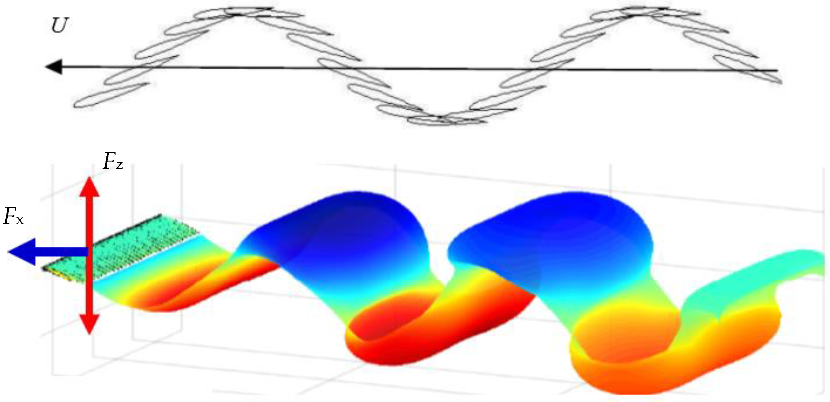
The flapping thruster operates as an unsteady hydrofoil combining heaving and pitching motion with a phase difference about 90 degrees, as depicted in Figure 1. The most important non-dimensional parameters are the Strouhal number $Str\hspace{0.17em}=\hspace{0.17em}2f{h}_0/U,$ where $f\hspace{0.17em}=\hspace{0.17em}\omega /2\pi$ is the frequency (with ω denoting the angular frequency), h₀ the heaving amplitude and $U$ the heaving amplitude and the forward travelling speed, the heave to chord ratio is $h_0/c$, the pitching amplitude is ${\theta }_0$, and the phase difference ψ between the foil heave and pitch oscillatory motions.

The case of the flapping wing of a large aspect ratio is considered in this study. For simplicity, using the unsteady hydrofoil theory (see, e.g., [21]) the lift force $F_L$ can be estimated as follows:

$$F_L\hspace{0.17em}=\hspace{0.17em}\frac{1}{2}\pi \rho UAH\left(AR\right)\hspace{0.17em}C\left(k\right)\left[U\theta \hspace{0.17em}-\hspace{0.17em}\dot{h}\hspace{0.17em}+\hspace{0.17em}\left(\frac{3}{4}\hspace{0.17em}-\hspace{0.17em}\frac{p}{c}\right)c\dot{\theta }\right]\hspace{0.17em}+\hspace{0.17em}\frac{\pi \rho c^2}{4}\left[\left(U\dot{\theta }\hspace{0.17em}-\hspace{0.17em}\ddot{h}\right)\hspace{0.17em}+\hspace{0.17em}c\left(\frac{1}{2}\hspace{0.17em}-\hspace{0.17em}\frac{p}{c}\right)\ddot{\theta }\right],$$

(1)

where $p/c$ is pitching axis location, $k=\omega c/\left(2U\right)$ is the reduced frequency, $C\left(k\right)$ is the Theodorsen function (lift deficiency factor), $A$ is the area of the foil, and $H=AR{\left(AR+2\right)}^{-1}$ is a 3D correction from lifting–line theory (elliptic wing). The instantaneous angle of attack $\alpha \left(t\right)$ is given by

$$a\left(t\right)\hspace{0.17em}=\hspace{0.17em}\theta \left(t\right)\hspace{0.17em}-\hspace{0.17em}{a}_b\left(t\right),\hspace{0.17em}\mathrm{where}\hspace{0.17em}{a}_b\left(t\right)\hspace{0.17em}=\hspace{0.17em}{\tan }^{-1}\left(\frac{\dot{h}}{U}\right)$$

(2)

where the foil pitching and heaving oscillatory motions are defined as follows:

$$\theta \left(t\right)\hspace{0.17em}=\hspace{0.17em}{\theta }_0\sin \left(\omega t\hspace{0.17em}+\hspace{0.17em}0.5\pi \right)\hspace{0.17em}\mathrm{and}\hspace{0.17em}h\left(t\right)\hspace{0.17em}=\hspace{0.17em}{h}_0\sin \left(\omega \hspace{0.17em}t\right)$$

(3)

The horizontal and vertical foil forces can be calculated as follows:

$$F_x\hspace{0.17em}=\hspace{0.17em}{F}_L\sin \left(\theta \right)\hspace{0.17em}-\hspace{0.17em}{F}_D\cos \left(\theta \right)$$

(4)

$$F_z\hspace{0.17em}=\hspace{0.17em}{F}_L\cos \left(\theta \right)\hspace{0.17em}+\hspace{0.17em}{F}_D\sin \left(\theta \right)$$

(5)

where $F_D=\frac{1}{2}\rho U^{2}A\hspace{0.17em}{C}_D\left(\mathrm{Re},\alpha \right)$ denotes a drag force that can be approximately considered by using a drag coefficient based on the Reynolds number and corrected for the angle of attack; see also [22].

The above simplified method provides us with a first estimation of the hydrodynamic loads that can be exploited in the sequel for estimating the noise generation and propagation by the oscillating foil. More accurate predictions for the hydrodynamic pressure field and loads associated with the operation of the flapping thruster can be derived by the implementation of unsteady BEM and CFD, as, e.g., presented by [23] taking also into account the effects of the free surface and incident waves. Moreover, systematic results and technical diagrams are provided by BEM [24].

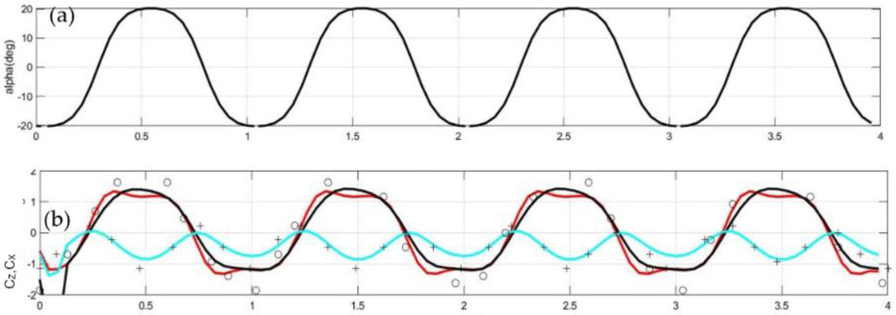
As an example, a flapping wing of $AR\hspace{0.17em}=\hspace{0.17em}6$ with symmetrical NACA0012 sections is considered and results concerning the time history of the dynamic angle of attack and the flapping thruster loads against non-dimensional time t/T, are presented in Figure 2. In this case, the flapping thruster operates at a Strouhal number $Str\hspace{0.17em}=\hspace{0.17em}2f{h}_0/U\hspace{0.17em}=\hspace{0.17em}0.23$, $h_0/c\hspace{0.17em}=\hspace{0.17em}0.75$, ${\theta }_0\hspace{0.17em}=\hspace{0.17em}23$ deg, where $f\hspace{0.17em}=\hspace{0.17em}\omega /2\pi$ is the frequency and T = 1/f the period, respectively, U is the foil steady travelling speed, $h_0$ the heaving amplitude, c is the chord in the centerplane of the wing and ${\theta }_0$ is the self-pitching amplitude about a pivot axis located at a distance of $c/3$ from the wing’s leading edge; for more details see Ref. [25].

In Figure 2a, the dynamic angle of attack is plotted and in Figure 2b the vertical (lift) force coefficient is shown by using a black line and the horizontal (thrust) force by using a cyan line, as calculated using the unsteady BEM method [26] and they are compared against the measured data [25] shown using symbols and the unsteady hydrofoil theory results using red lines. It is observed that the present method provides compatible predictions concerning the integrated quantities with unsteady hydrofoil theory and the experiment satisfactorily approximating the maxima of both the lift and thrust forces.

3. Noise Propagation in Free Space

The first integral approach for acoustic propagation is the Lighthill Acoustic Analogy [27]. The Ffowcs Williams and Hawkings (FW-H) [28] equation represents an extension of Lighthill’s Analogy, derived by rearranging the Navier–Stokes equations into a wave equation [29]. In recent years, this numerical approach is being used increasingly for applications to marine and maritime problems [30,31,32,33,34]. This method propagates the acoustic pressure by means of the analytical solution of the D’ Alembert’s equation in free space. Therefore, it cannot incorporate inhomogeneities as well as boundaries and interactions with surfaces. The pressure field and the forces produced by the flapping thruster motion, obtained using the BEM model described in the previous section, are used to calculate the dipole and monopole forcing terms associated with the initial boundary value problem governed by the FW-H equation. The acoustic model in free space is derived based on the Farassat formulation [35].

As the flapping thruster operates, it is subjected mainly to unsteady pressure loads. Low-frequency noise is caused by the fluctuations of foil pressure and volume flow disturbance due to oscillatory motion. The formulation for the acoustic pressure generated from rotating machinery based on the FW-H equation is described as follows:

$$\frac{1}{c^2}{\partial }_t^2{p}^{\prime }\left(x,t\right)\hspace{0.17em}-\hspace{0.17em}{\nabla }^2{p}^{\prime }\left(x,t\right)\hspace{0.17em}=\hspace{0.17em}{F}_{m\hspace{0.17em}}\hspace{0.17em}+\hspace{0.17em}{F}_{d\hspace{0.17em}}\hspace{0.17em}+\hspace{0.17em}{F}_q$$

(6)

where $c$ is the speed of sound in the medium ($1500\hspace{0.17em}\mathrm{m}/\mathrm{s} \le c \le 1550\hspace{0.17em}\mathrm{m}/\mathrm{s}$ for seawater), while the various terms on the right-hand side correspond to the acoustic monopole, dipole, and quadrupole source terms [36], respectively, and are defined as follows:

$$F_m\hspace{0.17em}=\hspace{0.17em}\frac{\partial }{\partial t}\hspace{0.17em}\left[\rho u_n\left|\nabla f\right|\delta \left(f\right)\right],\hspace{0.17em}{F}_d\hspace{0.17em}=\hspace{0.17em}-\frac{\partial }{\partial x_i}\hspace{0.17em}\left[l_i\left|\nabla f\right|\delta \left(f\right)\right],\hspace{0.17em}{F}_q\hspace{0.17em}=\hspace{0.17em}-\frac{{\partial }^2}{\partial x_i\partial x_j}\hspace{0.17em}\left[T_{ij}\hspace{0.17em}H\left(f\right)\right],$$

(7)

where $u_n$ is the normal velocity on the foil, $l_i$ represents the corresponding loads, and $T_{ij}$ denotes the stresses.

The quadrupole term becomes more important for high frequency and strongly transonic flow phenomena. Simplified models based on the above assumption have been presented by various authors, e.g., by [37] in the case of cavitating marine propellers. Considering that the speed of sound in water is much greater than the flow velocities and focusing on the low-frequency part of the generated noise spectrum, the contributions by the latter term are neglected in the present work. The Farassat formulation is employed offering an integral representation of the solution of Equation (6) forced by the monopole and dipole terms. This is a rearrangement of the basic conservation laws of mass and momentum into an inhomogeneous wave equation, where the different noise generation mechanisms are identified and expressed by separate source terms. Using the free-space Green’s function for the wave equation allows to write the two linear terms in an integral form. In the infinite homogeneous domain, the solution is given by thickness and loading components as follows:

$$p^{\prime }\left(x_0,t\right)\hspace{0.17em}=\hspace{0.17em}{p}_L^{\prime }\left(x_0,t\right)\hspace{0.17em}+\hspace{0.17em}{p}_T^{\prime }\left(x_0,t\right)$$

(8)

The loading term is given by

$$4\pi p_L^{\prime }\left(x_0,t\right)\hspace{0.17em}=\hspace{0.17em}-\hspace{0.17em}\frac{1}{c}\frac{d}{dt}{{\displaystyle \underset{f\hspace{0.17em}=\hspace{0.17em}0}{\int }\left[\frac{dpn\widehat{r}}{r\left(1-M_r\right)}\right]}}_{ret}dS\hspace{0.17em}+\hspace{0.17em}{{\displaystyle \underset{f\hspace{0.17em}=\hspace{0.17em}0}{\int }\left[\frac{dpn\widehat{r}}{r^2\left(1- M_r\right)}\right]}}_{ret}dS,$$

(9)

where $f\hspace{0.17em}=\hspace{0.17em}0$ indicates the moving surfaces, $dp$ denotes the pressure difference between the lower and upper sides of the foil surface, $M_r$ denotes the Mach number in the $r-$ direction, and the integrand is calculated at the retarded time. For relatively large distances of the observation point from the wing, we use the approximation

$$r\hspace{0.17em}=\hspace{0.17em}\left|x_0\hspace{0.17em}-\hspace{0.17em}x\right|\hspace{0.17em}\approx \hspace{0.17em}\left|x_0\hspace{0.17em}-\hspace{0.17em}{x}_T\left(t\right)\right|,\hspace{0.17em}\widehat{r}\hspace{0.17em}\approx \hspace{0.17em}\left(x_0\hspace{0.17em}-\hspace{0.17em}{x}_T\left(t\right)\right)/r$$

(10)

where $x_T$ denotes the center of lift and thrust force on the flapping wing. Using the fact that the Mach number is very small, the following simplification is derived from Equation (9):

$$p_L^{\prime }\left(x_0,t\right)\hspace{0.17em}=\hspace{0.17em}-\frac{1}{4\pi c}\frac{dF(t_r)}{dt}\frac{x_0-x_T\left(t_r\right)}{r^2}\hspace{0.17em}+\hspace{0.17em}\frac{1}{4\pi }F(t_r)\frac{x_0-x_T\left(t_r\right)}{r^3},$$

(11)

where $F(t_r)$ denotes the fluctuating unsteady part of the foil force, mainly composed from vertical (lift) and horizontal (thrust) forces, and $t_r\hspace{0.17em}=\hspace{0.17em}r/c$ denotes the retarded time between the observation point $x_0$ and the disturbance generating point $x_T$.

Similarly, for the thickness effect we have:

$$p_T^{\prime }(x_0,t)\hspace{0.17em}=\hspace{0.17em}\frac{\rho }{4\pi }\frac{\partial }{\partial t}{\displaystyle {\int }_{f=0}{\left[\frac{u_n}{r(1-M_r)}\right]}_{ret}}dS,$$

(12)

which is approximated by

$$p_T^{\prime }(x_0,t)\hspace{0.17em}\approx \hspace{0.17em}\frac{\rho }{4\pi }\frac{d^2{Q}_c(t_r)}{d{t}^2}\frac{1}{\left|x_0-x_Q(t_r)\right|}$$

(13)

where $x_Q(t_r)$ is the center of volume $Q_c$ displaced by the foil. In the case of an unsteady cavitating foil thruster, the latter term will also include the volume fluctuation of the sheet and tip vortex cavities and bubbles which in several cases, e.g., flapping foils and marine propellers, has a periodic or nearly periodic character.

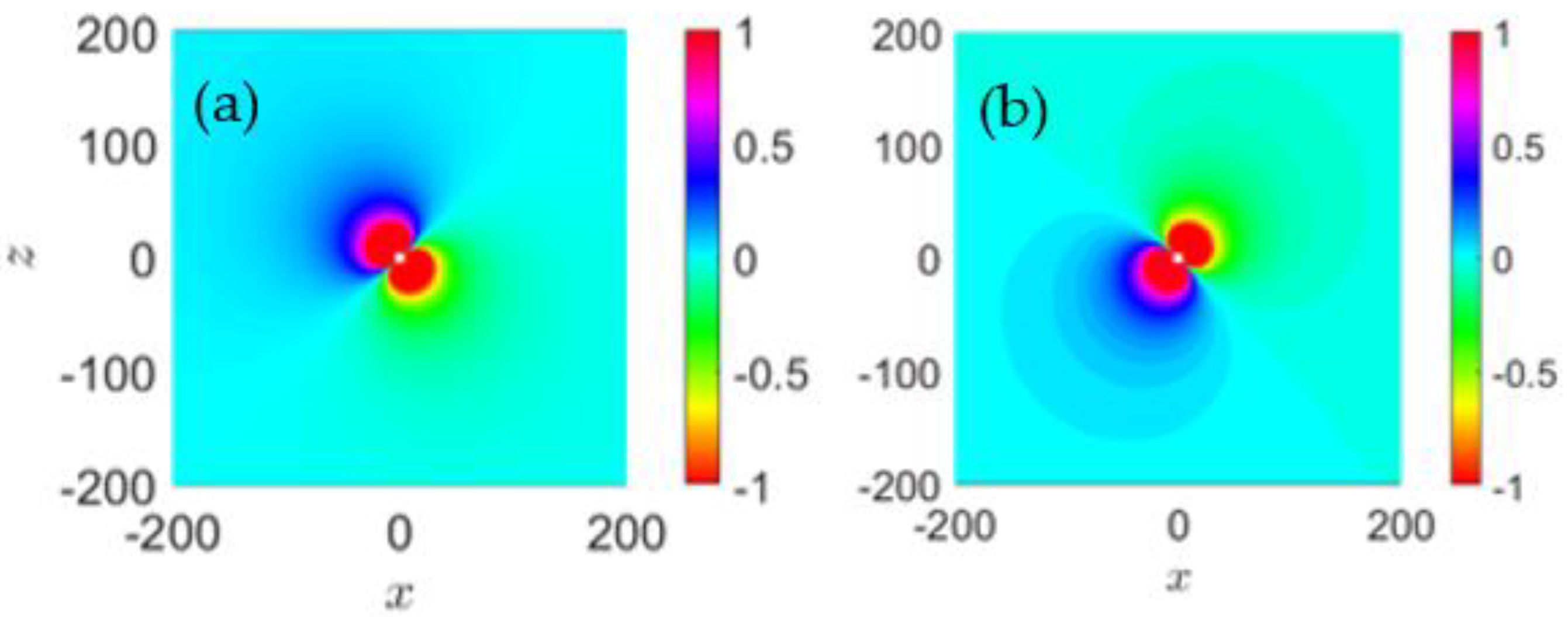
Indicative results concerning the calculated acoustic field in free space generated by the flapping thruster operating in water ($c\hspace{0.17em}=\hspace{0.17em}1500$ m/s), as obtained using the above equations, are presented in Figure 3. In particular, the case of the foil of Figure 1 is considered, flapping at $Str\hspace{0.17em}=\hspace{0.17em}0.23$, $h_0/c\hspace{0.17em}=\hspace{0.17em}0.75$ and ${\theta }_0\hspace{0.17em}=\hspace{0.17em}23\hspace{0.17em}\mathrm{deg}$, and the acoustic field is calculated using Equations (11) and (13) using the hydrodynamic loads of Figure 2b. The result in the near field is plotted at two instants, when the nose of the flapping thruster is directed upwards and downwards, respectively, and the field is normalized with respect to its value at the distance of 1 m from the source point.

In the case of periodic signals, the acoustic force $F(t)$ and cavity volume data $Q\left(t\right)$ can be represented by the Fourier series and using the results in conjunction with the Green’s function of the Helmholtz equation in free space:

$$G(x,x_0)\hspace{0.17em}=\hspace{0.17em}\frac{1}{4\pi }\frac{e^{i{k}_n\left|x-x_0\right|}}{\left|x-x_0\right|}$$

(14)

and its derivative:

$${\nabla }_{x_0}G(x,x_0)\hspace{0.17em}=\hspace{0.17em}\frac{e^{i{k}_n\left|x-x_0\right|}}{4\pi {\left|x-x_0\right|}^2}\left(\frac{\left(x-x_0\right)}{\left|x-x_0\right|}-i{k}_n\left(x-x_0\right)\right)$$

(15)

we find that the expressions provided by Equations (11) and (13) are the time-domain equivalent of the solution of the Helmholtz equation with complex monopole and dipole source intensities provided by:

$$Q_{n\hspace{0.17em}}\hspace{0.17em}=\hspace{0.17em}-\rho n^2{\omega }^2\left(Q_n^c\hspace{0.17em}-\hspace{0.17em}i{Q}_n^s\right), X_{n\hspace{0.17em}}\hspace{0.17em}=\hspace{0.17em}{X}_n^c\hspace{0.17em}-\hspace{0.17em}i{X}_n^s, Z_{n\hspace{0.17em}}\hspace{0.17em}=\hspace{0.17em}{Z}_n^c-i{Z}_n^s,$$

(16)

that is

$$p_m\left(x,t\right)\hspace{0.17em}=\hspace{0.17em}\frac{1}{4\pi }\mathrm{Re}\left({\displaystyle \sum _n{Q}_n}\frac{e^{i{k}_n\left|x\hspace{0.17em}-\hspace{0.17em}{x}_0\right|}}{\left|x\hspace{0.17em}-\hspace{0.17em}{x}_0\right|}{e}^{-i{\omega }_{n}t}\right)$$

(17)

$$p_d\left(x,t\right)\hspace{0.17em}=\hspace{0.17em}\frac{1}{4\pi }\mathrm{Re}\left({\displaystyle \sum _n\left(X_{n}i\hspace{0.17em}+\hspace{0.17em}{Z}_{n}k\right)}\frac{e^{i{k}_n\left|x\hspace{0.17em}-\hspace{0.17em}{x}_0\right|}}{4\pi {\left|x\hspace{0.17em}-\hspace{0.17em}{x}_0\right|}^2}\left(\frac{\left(x\hspace{0.17em}-\hspace{0.17em}{x}_0\right)}{\left|x\hspace{0.17em}-\hspace{0.17em}{x}_0\right|}\hspace{0.17em}-\hspace{0.17em}i{k}_n\left(x\hspace{0.17em}-\hspace{0.17em}{x}_0\right)\right)e^{-i{\omega }_{n}t}\right)$$

(18)

The above equations provide us with the expression of the complex monopole and dipole source terms at the basic frequency and its multiples, as provided by the hydrodynamic flapping foil responses described above. The above are sufficient for the study of acoustic noise generation and propagation from the flapping thruster in free space (unbounded domain). However, in the case of a bounded domain as it happens in underwater acoustics where the propagation is affected by the presence of the free surface and seabed boundary, the above results can be used to determine the source intensity. Subsequently, the propagation of noise emitted by the flapping foil in the ocean acoustic waveguide is obtained by formulating and numerically solving the forced acoustic equation, considering refraction, reflection, and scattering effects, as described in the next section.

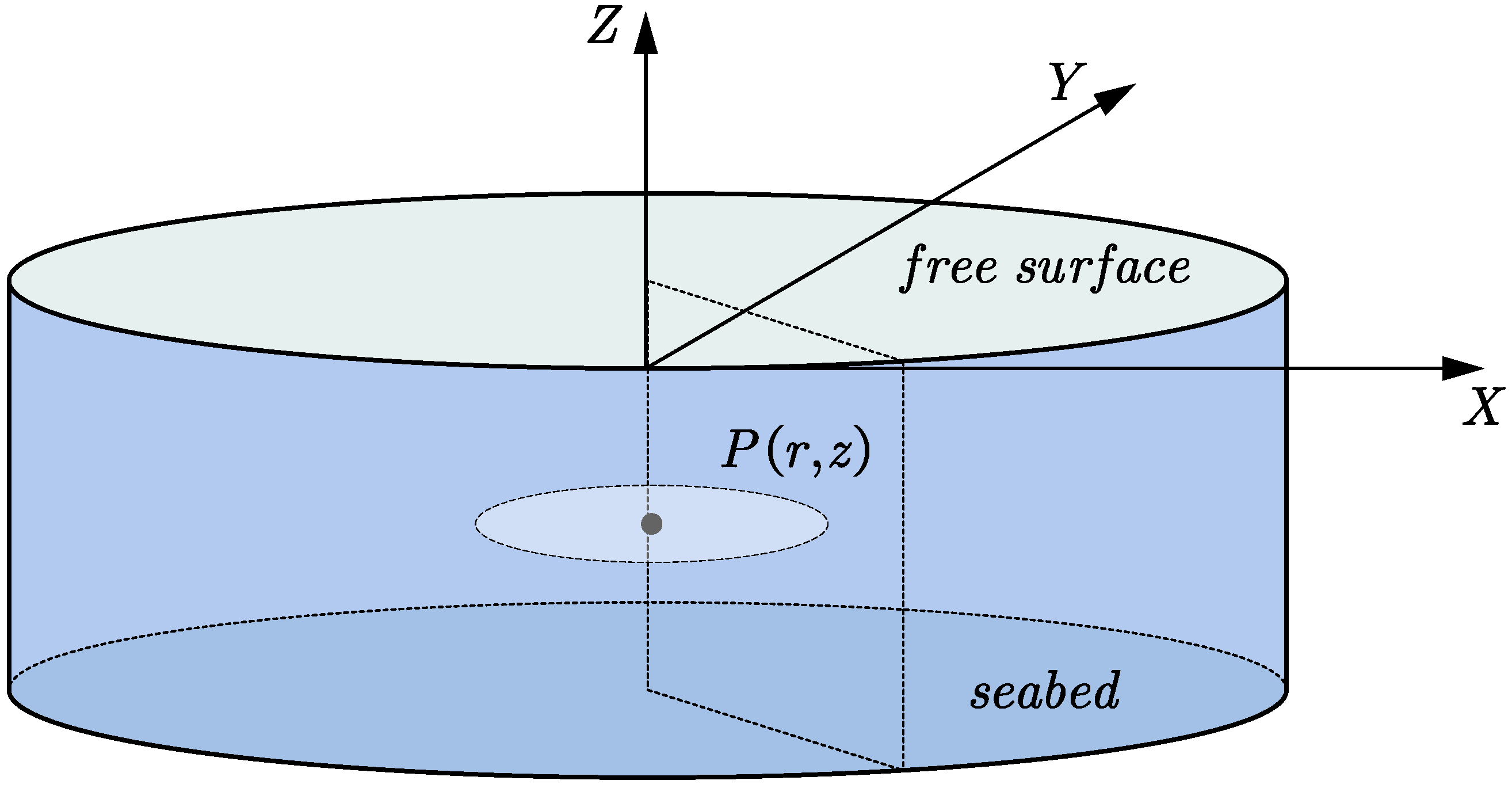
4. Noise Propagation in the 3D Ocean Acoustic Waveguide

We consider the ocean acoustic waveguide limited above by the sea surface and below by the seabed; see Figure 4. Both Cartesian $x\hspace{0.17em}=\hspace{0.17em}\left(x,y,z\right)$ and cylindrical coordinates $x\hspace{0.17em}=\hspace{0.17em}\left(r\hspace{0.17em}=\hspace{0.17em}\sqrt{{\left(x\hspace{0.17em}-\hspace{0.17em}{x}_s\right)}^2\hspace{0.17em}+\hspace{0.17em}{\left(y\hspace{0.17em}-\hspace{0.17em}{y}_s\right)}^2\hspace{0.17em}},\hspace{0.17em}\theta \hspace{0.17em}=\hspace{0.17em}{\tan }^{-1}\left(\left(y\hspace{0.17em}-\hspace{0.17em}{y}_s\right)/\left(x\hspace{0.17em}-\hspace{0.17em}{x}_s\right)\right),\hspace{0.17em}z\right)$ are used in the formulation with the origin at a point located above the acoustic source on the free surface. For the considered problem, the hydroacoustic model is extended to treat the bounded waveguide featuring the inhomogeneity of parameters. To address the latter complexity, an axisymmetric cylindrical environment is used to account for the geometrical spreading. The developed numerical method is based on a finite difference scheme in the time domain (FDTD) able to incorporate the effects imposed by the free surface, seabed boundaries, as well as a variable sound speed profile. For the open radiation boundaries, a PML reformulation of the acoustic wave equation for the truncated inhomogeneous ocean waveguide is presented, and subsequently employed in the numerical scheme.

4.1. The 3D Acoustic Problem in a Constant Depth

The forcing terms associated with the monopole and vertical dipole terms are clearly azimuthally symmetric and in an environment where the parameters do not depend on θ the generated fields are also azimuthally symmetric. In the case of excitation by the horizontal dipole source, the forcing term is explicitly dependent on θ, and we approximately assume that the same holds also for the generated field in the above environments. Using the above facts, assuming the azimuthal symmetry the hyperbolic acoustic equation expressed in cylindrical coordinates $x\hspace{0.17em}=\left(r,\theta ,z\right)$ takes the following form:

$$\frac{1}{c^2\left(x\right)}{\partial }_t^{2}p\left(x,t\right)\hspace{0.17em}-\hspace{0.17em}\left(\frac{1}{r}{\partial }_r\left(r{\partial }_{r}p\left(x,t\right)\right)\hspace{0.17em}+\hspace{0.17em}{\partial }_z^{2}p\left(x,t\right)\right)\hspace{0.17em}=\hspace{0.17em}F\left(x,t\right),\hspace{0.17em}r\in I{R}_0^{+},\hspace{0.17em}-h<z<0$$

(19)

$$p\left(x,t\right){|}_{x\in S_F}\hspace{0.17em}=\hspace{0.17em}0,\hspace{0.17em}r\in I{R}_0^{+},\hspace{0.17em}z\hspace{0.17em}=\hspace{0.17em}0,$$

(20)

$${\partial }_{n}p\left(x,t\right){|}_{x\in S_B}\hspace{0.17em}=\hspace{0.17em}0,\hspace{0.17em}r\in I{R}_0^{+},\hspace{0.17em}z\hspace{0.17em}=\hspace{0.17em}-h,$$

(21)

The homogeneous Dirichlet boundary condition is used for modeling the free surface Equation (20), and for simplicity the seabed is modeled as a hard boundary using the Neumann boundary condition, Equation (21). In Equation (19), $F\left(x;t\right)$ is the forcing term that includes both dipole and monopole sources, and $c\left(x\right)$ denotes the variable sound speed. Since the hydroacoustic problem is inherently defined in the infinite ocean waveguide, the numerical methods need to incorporate appropriate termination conditions that ensure field radiation at the numerically truncated boundary.

The solution of problem Equations (19)–(21) will be based on the time integration technique using a finite-difference numerical scheme. Expanding the idea regarding the determination of the monopoles and dipoles in the previous section, we need to formulate suitable expressions for the acoustic sources into the time domain produced by the Helmholtz equation, as well. Thus, the $F\left(x;t\right)$ will be determined in the source near field by the Green’s function of the Helmholtz equation in the bounded waveguide and its derivatives, which will be presented in Section 4.2. Additionally, the outward radiation condition will be satisfied by a Perfectly Matched Layer (PML) technique and will be discussed in detail in Section 4.3. Finally, the FDTD–PML numerical scheme and the numerical results and the corresponding verifications with analytical solutions will be presented Section 4.4.

4.2. Determination of the Source Near-Field Data in the Acoustic Waveguide

The singular nature of the cylindrical Laplacian operator, along with the presence of point singularities (monopole and dipole sources) pose difficulties in numerical implementation. In the present work, these challenges are overcome by the enforcement of the field data in the near-field region. In this procedure, the original domain is divided into two subdomains, the computational domain $\mathsf{\Omega }$ and the residual domain D (or relaxation zone) as shown in Figure 5. The problem is solved analytically in $D=\left\{r<r_{REL},\hspace{0.17em}-h<z<0,\hspace{0.17em}0\le \theta <2\pi \right\}$ for monopole and dipole force terms, and the data concerning the acoustic field are used to propagate the solution numerically in $\mathsf{\Omega }=\left\{r_{REL}<r<r_{PML},\hspace{0.17em}-h<z<0,\hspace{0.17em}0\le \theta <2\pi \right\}$ solving the problem consisting of Equations (19)–(21).

For this purpose, the Green’s function $G\left(x|x_s\right)$ of the Helmholtz equation, satisfying the free-surface and hard seabed boundary conditions, is implemented in the near-source subregion of the waveguide:

$${\nabla }^{2}G\hspace{0.17em}+\hspace{0.17em}{k}^{2}G\hspace{0.17em}=\hspace{0.17em}-\delta \left(x-x_S\right)$$

(22)

where $\delta \left(x-x_S\right)$ is the Dirac delta function.

The corresponding expressions modeling the dipole terms associated with the lift and thrust foil forces are defined as solutions of:

$${\nabla }^2{G}_{l,m,n}\hspace{0.17em}+\hspace{0.17em}{k}^2{G}_{l,m,n}\hspace{0.17em}=\hspace{0.17em}\frac{{\partial }^{l+m+n}}{\partial x^l\partial y^m\partial z^n}\delta \left(x-x_S\right)$$

(23)

and are obtained as:

$$G_{l,m,n}\hspace{0.17em}=\hspace{0.17em}{\left(-1\right)}^{l+m+n}\frac{{\partial }^{l+m+n}}{\partial x^l\partial y^m\partial z^n}G\left(x|x_s\right)$$

(24)

where $G$ is the Green’s function and $x_s$ denotes the position of the singularity; see [38]. Thus, the present monopole and dipole (horizontal and vertical) sources data in the near-field region are obtained from the corresponding Green’s function of the Helmholtz equation by using the harmonic time dependence, i.e., $G\left(x|x_s;t\right)\hspace{0.17em}=\hspace{0.17em}\hspace{0.17em}\mathrm{Re}\left\{G\left(x|x_s;\omega \right)e^{-i\omega t}\right\}.$

Next, we consider the source region to be range independent and thus the monopole source denoted by $G_M\left(x|x_s;\omega \right)$ is obtained using separation of the variables as follows [12]:

$$G_M\left(x|x_s;\omega \right)\hspace{0.17em}\hspace{0.17em}=\hspace{0.17em}\frac{i}{4}{\displaystyle \sum _{m=1}^{\infty }{\tilde{Z}}_m}\left(z_s\right){\tilde{Z}}_m\left(z\right)H_0^{\left(1\right)}\left(k_{rm}r\right)$$

(25)

where the normalized vertical eigenfunctions are:

$${\tilde{Z}}_n\left(z\right)\hspace{0.17em}=\hspace{0.17em}{Z}_n\left(z\right)/\Vert Z_n\Vert \hspace{0.17em},\hspace{0.17em}{\displaystyle {\int }_{-h}^0{\tilde{Z}}_m}\left(z\right){\tilde{Z}}_n\left(z\right)dz\hspace{0.17em}=\hspace{0.17em}{\delta }_{nm}$$

(26)

where ${\delta }_{nm}\hspace{0.17em}$ is the Kronecker delta and solutions to the corresponding Vertical Eigenvalue Problem (VEP) are obtained as:

$$\frac{d^2{Z}_m\left(z\right)}{d{z}^2}\hspace{0.17em}+\hspace{0.17em}\left[\frac{{\omega }^2}{c^2\left(z\right)}\hspace{0.17em}-\hspace{0.17em}{k}_{rm}^2\right]Z_m\left(z\right)\hspace{0.17em}=\hspace{0.17em}0$$

(27)

with boundary conditions:

$$Z_m\left(z\hspace{0.17em}=\hspace{0.17em}0\right)\hspace{0.17em}=\hspace{0.17em}0,\hspace{0.17em}\hspace{0.17em}\mathrm{on} \mathrm{the} \mathrm{free} \mathrm{surface}$$

(28)

$$\hspace{0.17em}\frac{d{Z}_m}{dz}{|}_{z=-h}\hspace{0.17em}=\hspace{0.17em}0,\hspace{0.17em}\hspace{0.17em}\mathrm{on} \mathrm{the} \mathrm{hard} \mathrm{bottom}$$

(29)

where $k_{rm}$ represents the eigenvalues. In the case of a homogeneous environment, the VEP is solved analytically, whereas in the case of a vertical sound speed profile the Sturm–Liouville problem is solved numerically by, e.g., the Finite Difference Method (see [12]).

In the case of a sound field generated by a horizontal dipole (associated with the foil thrust forcing) and a vertical dipole (associated with the lift force) the corresponding expressions are as follows:

$$G_H\hspace{0.17em}\left(x|x_s;\omega \right)\hspace{0.17em}=\hspace{0.17em}{\partial }_{x_s}{G}_M\hspace{0.17em}=\hspace{0.17em}-\frac{i}{4}{\displaystyle \sum _{m=1}^{\infty }{\tilde{Z}}_m}\left(z_s\right){\tilde{Z}}_m\left(z\right)k_{rm}{H}_1^{\left(1\right)}\left(k_{rm}r\right){\partial }_{x_s}r\hspace{0.17em}=\hspace{0.17em}\frac{i\cos \theta }{4}{\displaystyle \sum _{m=1}^{\infty }{\tilde{Z}}_m}\left(z_s\right){\tilde{Z}}_m\left(z\right)H_1^{\left(1\right)}\left(k_{rm}r\right),\hspace{0.17em}$$

(30)

$$G_V\hspace{0.17em}\left(x|x_s;\omega \right)\hspace{0.17em}=\hspace{0.17em}{\partial }_{z_s}{G}_M\hspace{0.17em}=\hspace{0.17em}\frac{i}{4}{\displaystyle \sum _{m=1}^{\infty }{\tilde{Z}}_m^{\prime }}\left(z_s\right){\tilde{Z}}_m\left(z\right)H_0^{\left(1\right)}\left(k_{rm}r\right),$$

(31)

where ${\partial }_{x_s}r\hspace{0.17em}=\hspace{0.17em}\left(x\hspace{0.17em}-\hspace{0.17em}{x}_s\right)/r\hspace{0.17em}=\hspace{0.17em}\cos \theta$ and $\theta$ is the azimuthal angle.

The above analytical expressions obtained using the normal-mode expression of the Green’s function of the Helmholtz equation and its derivatives in $D$ are converted to the time domain as follows

$$F\left(x,t\right)\hspace{0.17em}=\hspace{0.17em}\mathrm{Re}\left({\displaystyle \sum _n\left(Q_{n}G\left(x|x_s;{\omega }_n\right)+X_n{G}_H\hspace{0.17em}\left(x|x_s;\omega \right)+Z_n{G}_H\hspace{0.17em}\left(x|x_s;\omega \right)\right)}\hspace{0.17em}{e}^{-i{\omega }_{n}t}\right),\hspace{0.17em}r<r_{REL},$$

(32)

in order to be used to enforce near-source field data in Equation (19) by applying a relaxation scheme. Subsequently, the problem is numerically solved in cylindrical coordinates by using a Finite Difference Time Domain solver, in conjunction with a Perfectly Matched Layer technique for the satisfaction of the radiation condition (FDTD–PML), which is described in detail in the next subsections.

4.3. Incorporation of the Perfectly Matched Layer into the Acoustic Equation

To address the need of modeling general boundaries and inhomogeneities in a large domain, an absorbing boundary technique dissipating outgoing waves with minimum backscattering and without excessive computational cost is considered; see, e.g., [39]. In the present work, a Perfectly Matched Layer (PML) method is used based on Berenger’s [39] original PML formulation. In general, PML formulations in the time domain reorganize the second-order wave equation into a system of first-order equations, by introducing pseudo-variables [40,41,42,43,44,45]. Alternatively, the direct treatment of the second-order wave problem has been proposed by [46,47]. Finally, optimal PML formulations for the Helmholtz equation are proposed in [48,49].

In this work, the derivation of the PML method for a 3D cylindrical waveguide is based on Berenger’s model. The basic step consists of applying a complex change in variables as follows (coordinate stretching):

$$\left\{\begin{array}{c}{\partial }_r\\ {\partial }_z\end{array}\right\}\hspace{0.17em}=\hspace{0.17em}\left(\begin{array}{cc}{\gamma }_r^{-1}& 0\\ 0& {\gamma }_z^{-1}\end{array}\right)\left\{\begin{array}{c}{\partial }_r\\ {\partial }_z\end{array}\right\}$$

(33)

However, in our case only r-stretching is required

$${\gamma }_r\left(r\right)\hspace{0.17em}=\hspace{0.17em}\{\begin{array}{cc}1,& r\hspace{0.17em}<\hspace{0.17em}{r}_{PML}\hspace{0.17em}-\hspace{0.17em}L,\hfill \\ 1\hspace{0.17em}+\hspace{0.17em}\frac{i}{\omega }{\sigma }_r\left(r\right),& r\hspace{0.17em}\ge \hspace{0.17em}{r}_{PML}\hspace{0.17em}-\hspace{0.17em}L\hfill \end{array},\hspace{0.17em}\mathrm{and}\hspace{0.17em}{\gamma }_z\left(r\right)\hspace{0.17em}=\hspace{0.17em}1,$$

(34)

where L denotes the PML thickness. In the present case, the variable absorption coefficient within the layer is denoted as ${\sigma }_r$ and is defined as a function of $r$, as it will be provided in the sequel.

Equation (19) can be expressed as a system of equations by introducing the pseudo-variable ${\partial }_{t}w\hspace{0.17em}\hspace{0.17em}=\hspace{0.17em}\nabla p\hspace{0.17em}$ and the following system is derived,

$$\{\begin{array}{l}\frac{1}{c^2\left(x\right)}\hspace{0.17em}{{\partial }^2}_t\hspace{0.17em}-\hspace{0.17em}{\partial }_r^{2}p\left(x,t\right)\hspace{0.17em}-\hspace{0.17em}{\partial }_z^{2}p\left(x,t\right)\hspace{0.17em}+\hspace{0.17em}{\partial }_{t}p\left(x,t\right)\left({\sigma }_r+{\sigma }_z\right)+\\ \hspace{0.17em}\hspace{0.17em}+\frac{1}{c^2\left(x\right)}{\sigma }_r{\sigma }_{z}p\left(x,t\right)\hspace{0.17em}+\hspace{0.17em}\nabla \cdot diag\left(B\left(x\right)\hspace{0.17em}A\left(x\right)\right)\hspace{0.17em}-\hspace{0.17em}\frac{1}{r}\left({\partial }_{r}p \hspace{0.17em}-\hspace{0.17em}{\sigma }_r{v}_r\right)\hspace{0.17em}\hspace{0.17em}=\hspace{0.17em}\hspace{0.17em}F\left(x,t\right)\\ \frac{\partial w}{\partial t}\hspace{0.17em}\hspace{0.17em}=\hspace{0.17em}\hspace{0.17em}\nabla p\left(x,t\right)\hspace{0.17em}-\hspace{0.17em}diag\left(B\left(x\right)A\left(x\right)\right)\hspace{0.17em},\end{array}$$

(35)

where ${\rm B}\left(x\right)\hspace{0.17em}=\hspace{0.17em}\left[\begin{array}{cc}{\sigma }_r& 0\\ 0& {\sigma }_z\end{array}\right],\hspace{0.17em}A\left(x\right)\hspace{0.17em}=\hspace{0.17em}\left[\begin{array}{cc}{w}_r& 0\\ 0& w_z\end{array}\right]$ and $w\hspace{0.17em}=\hspace{0.17em}\left(w_r,w_z\right)$.

The damping terms ${\sigma }_r,\hspace{0.17em}{\sigma }_z$ are assumed to be non-negative functions. Within the absorbing layer, where ${\sigma }_r,\hspace{0.17em}{\sigma }_z\hspace{0.17em}>\hspace{0.17em}0$, the wavelike solutions are transformed into exponentially decaying ones. In the computational domain of interest, the above terms vanish (${\sigma }_x\hspace{0.17em}=\hspace{0.17em}{\sigma }_z\hspace{0.17em}=\hspace{0.17em}0$) and the system reduces to the 3D cylindrical acoustic equation. The numerical solution is obtained using a finite-difference discretization and time marching integration. Noticing the excitation foil forces in Figure 2 and the different main frequency and harmonics involved in the time series of lift and thrust, the time-domain scheme is considered more efficient for the propagation of the source data.

4.4. The FDTD–PML Model

The aim of this section is to introduce the Finite Difference Time Domain–Perfectly Matched Layer (FDTD–PML) solver used as a propagator, along with the relaxation scheme described above, for discretizing the system of Equation (35) and enforcing the source data, respectively. All spatial derivatives are discretized with centered finite differences, which guarantees second-order approximation in space. For time discretization, centered finite differences for the first- and second-order time derivatives on a uniform mesh is also employed.

Let $\Delta t>0$ denote the time step size and $\Delta r,\Delta z>0$ denote the spatial mesh sizes in the in the $r,z$ directions, respectively. Denoting the nth time step as $t_n\hspace{0.17em}=\hspace{0.17em}n\Delta t$ and the spatial nodes $r_i\hspace{0.17em}=\hspace{0.17em}i\Delta r,\hspace{0.17em}{z}_i\hspace{0.17em}=\hspace{0.17em}j\Delta z$, the Laplacian is discretized as follows:

$${{\nabla }^2}_n{p}_{i,j}^n\hspace{0.17em}=\hspace{0.17em}\frac{p_{i+1,j}^n\hspace{0.17em}-\hspace{0.17em}2p_{i,j}^n\hspace{0.17em}+\hspace{0.17em}{p}_{i-1,j}^n}{\Delta r^2}\hspace{0.17em}+\hspace{0.17em}\frac{1}{r_{i,j}}\frac{p_{i+1,j}^n\hspace{0.17em}-\hspace{0.17em}{p}_{i-1,j}^n}{2\Delta r}\hspace{0.17em}+\hspace{0.17em}\frac{p_{i,j+1}^n\hspace{0.17em}-\hspace{0.17em}2p_{i,j}^n\hspace{0.17em}+\hspace{0.17em}{p}_{i,j-1}^n}{\Delta z^2}$$

(36)

The first- and second-order time derivatives are provided, respectively, as,

$${\partial }_t^2{p}_{i,j}^n\hspace{0.17em}=\hspace{0.17em}\frac{p_{i,j}^{n+1}\hspace{0.17em}-\hspace{0.17em}2p_{i,j}^n\hspace{0.17em}+\hspace{0.17em}{p}_{i,j}^{n-1}\hspace{0.17em}}{\Delta t^2},\hspace{0.17em}{\partial }_t{p}_{i,j}^n\hspace{0.17em}=\hspace{0.17em}\frac{p_{i,j}^{n+1}\hspace{0.17em}-\hspace{0.17em}{p}_{i,j}^{n-1}}{2\Delta t}$$

(37)

Next, by substituting Equations (36) and (37) into the modified wave equation, Equation (35), we obtain the following discrete scheme:

$$\begin{array}{l}p{\hspace{0.17em}}_{i,j}^{n+1}\hspace{0.17em}=\hspace{0.17em}c{\hspace{0.17em}}_{i,j}^2\Delta t{\hspace{0.17em}}^2\frac{1}{\left(1+c_{i,j}^2\frac{\Delta t}{2}\left({\sigma }_r+{\sigma }_z\right)\right)}\hspace{0.17em}[\hspace{0.17em}-\hspace{0.17em}\frac{1}{c{\hspace{0.17em}}_{i,j}^2\Delta t{\hspace{0.17em}}^2}{p}_{i,j}^{n-1}\hspace{0.17em}\left(\hspace{0.17em}1\hspace{0.17em}-\hspace{0.17em}c{\hspace{0.17em}}_{i,j}^2\hspace{0.17em}\frac{\Delta t}{2}\hspace{0.17em}\left({\sigma }_r\hspace{0.17em}+\hspace{0.17em}{\sigma }_z\right)\hspace{0.17em}\right)+\\ \hspace{0.17em}\hspace{0.17em}\hspace{0.17em}\hspace{0.17em}\hspace{0.17em}\frac{1}{c{\hspace{0.17em}}_{i,j}^2\Delta t{\hspace{0.17em}}^2}\hspace{0.17em}2p{\hspace{0.17em}}_{i,j}^n\hspace{0.17em}\left(\hspace{0.17em}1\hspace{0.17em}-\hspace{0.17em}0.5\hspace{0.17em}c{\hspace{0.17em}}_{i,j}^2\Delta t{\hspace{0.17em}}^2{\sigma }_r{\sigma }_z\hspace{0.17em}-\hspace{0.17em}\frac{1}{\Delta r^2}\hspace{0.17em}-\hspace{0.17em}\frac{1}{\Delta z^2}\hspace{0.17em}\right)\hspace{0.17em}-\hspace{0.17em}\nabla \cdot diag\left(B\left(x\right)A\left(x\right)\right)+\\ \hspace{0.17em}\hspace{0.17em}\hspace{0.17em}p{\hspace{0.17em}}_{i+1,j}^n\left(\frac{1}{r_{i,j}2\Delta r}\hspace{0.17em}+\hspace{0.17em}\frac{1}{\Delta r^2}\right)\hspace{0.17em}+\hspace{0.17em}p{\hspace{0.17em}}_{i-1,j}^n\left(\frac{1}{\Delta r^2}\hspace{0.17em}-\hspace{0.17em}\frac{1}{r_{i,j}2\Delta r}\right)\hspace{0.17em}+\hspace{0.17em}\left(\hspace{0.17em}\frac{p{\hspace{0.17em}}_{i,j+1}^n\hspace{0.17em}+\hspace{0.17em}p{\hspace{0.17em}}_{i,j-1}^n}{\Delta z^2}\right)\hspace{0.17em}+\hspace{0.17em}F{\hspace{0.17em}}_{i,j}]\hspace{0.17em}. \end{array}$$

(38)

The above scheme is used explicitly together with the system of equations which includes the pseudovariable $w\hspace{0.17em}=\hspace{0.17em}\left(w_r,w_z\right)$,

$$w\hspace{0.17em}=\hspace{0.17em}\left({\nabla }_{i,j}p\left(x,t\right)-diag\left(B\left(x\right)A\left(x\right)\right)\right)\Delta t$$

(39)

where ${\nabla }_{i,j}={\left({\partial }_r,{\partial }_z\right)}_{i,j}$ denotes the finite difference approximation of the gradient on the i,j grid point of the spatial mesh.

In the sequel, we restrict our attention to problems formulated at the given azimuthal angle $\theta$ and the PML subregions correspond to large $r>r_{PML}$. Although the PML has very good properties in its continuous form, a number of factors including the spatial discretization, the PML thickness $L$, the mesh density, and the absorption function need to be optimized in the discrete version. These aspects have been studied for classical wave problems in various works [50,51,52]. Within the context of the present work, the absorbing function takes Berenger’s [40] polynomial form,

$${\sigma }_r\left(r\right)\hspace{0.17em}=\hspace{0.17em}{\sigma }_0{\left(L^{-1}\left|r\hspace{0.17em}-\hspace{0.17em}{r}_{PML}+L\right|\right)}^m\hspace{0.17em},$$

(40)

where ${\sigma }_0$ is a positive parameter, $L$ is the thickness of the layer, and $m$ is the polynomial degree. Suitable choices for ${\sigma }_0$, $L$, and $m$ are required to ensure minimal numerical solution contamination within the region of interest through interface reflection as well as back propagation from the fictitious termination boundary. In the present work, $L$ is selected to be of the order of characteristic acoustic wavelength and $m\hspace{0.17em}=\hspace{0.17em}3$.

As already discussed in the previous subsection, the source, the free-surface, and the hard seabed data are enforced by a relaxation scheme at each time step providing the field data in the notes

$$p_{i,j}^n\hspace{0.17em}=\hspace{0.17em}{G}_{M,H,V}\left(r_{i,j}^{\left(N\right)}\hspace{0.17em},z_{i,j}^{\left(N\right)};t\hspace{0.17em}=\hspace{0.17em}{t}_n\right)$$

(41)

for (i,j) in the source field region,

$$p_{i,j}^n\hspace{0.17em}=\hspace{0.17em}0,\hspace{0.17em}\hspace{0.17em}\mathrm{for}\hspace{0.17em}\left(r_{i,j}^{\left(FS\right)}\hspace{0.17em},z_{i,j}^{\left(FS\right)}\hspace{0.17em}=\hspace{0.17em}0;t\hspace{0.17em}=\hspace{0.17em}{t}_n\right)$$

(42)

$$p_{i,1}^n\hspace{0.17em}-p_{i,2}^n\hspace{0.17em}=\hspace{0.17em}0,\hspace{0.17em}\hspace{0.17em}\mathrm{for}\hspace{0.17em}\left(r_{i,j}^{\left(FS\right)}\hspace{0.17em},z_{i,j}^{\left(FS\right)}\hspace{0.17em}=\hspace{0.17em}-h;t\hspace{0.17em}=\hspace{0.17em}{t}_n\right)$$

(43)

where $h$ denotes the waveguide depth.

5. Numerical Results and Discussion

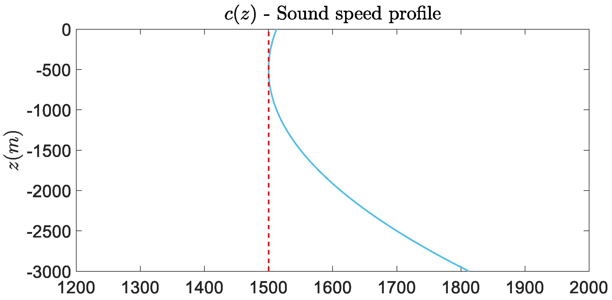
A series of numerical results, obtained by means of the developed FDTD–PML scheme, including the free surface and seabed effects, are presented in this section. Acoustic propagation is considered in both homogeneous environments, featuring constant velocity $c\hspace{0.17em}=\hspace{0.17em}1500m/s$, as well as in more realistic cases where the velocity exhibits vertical variation. The employed variable velocity profile is shown in Figure 6 and described as

$$c\left(z\right)\hspace{0.17em}=\hspace{0.17em}5\cdot {10}^{-5}{z}^2\hspace{0.17em}+\hspace{0.17em}0.05z\hspace{0.17em}+\hspace{0.17em}1.5125\cdot {10}^3$$

(44)

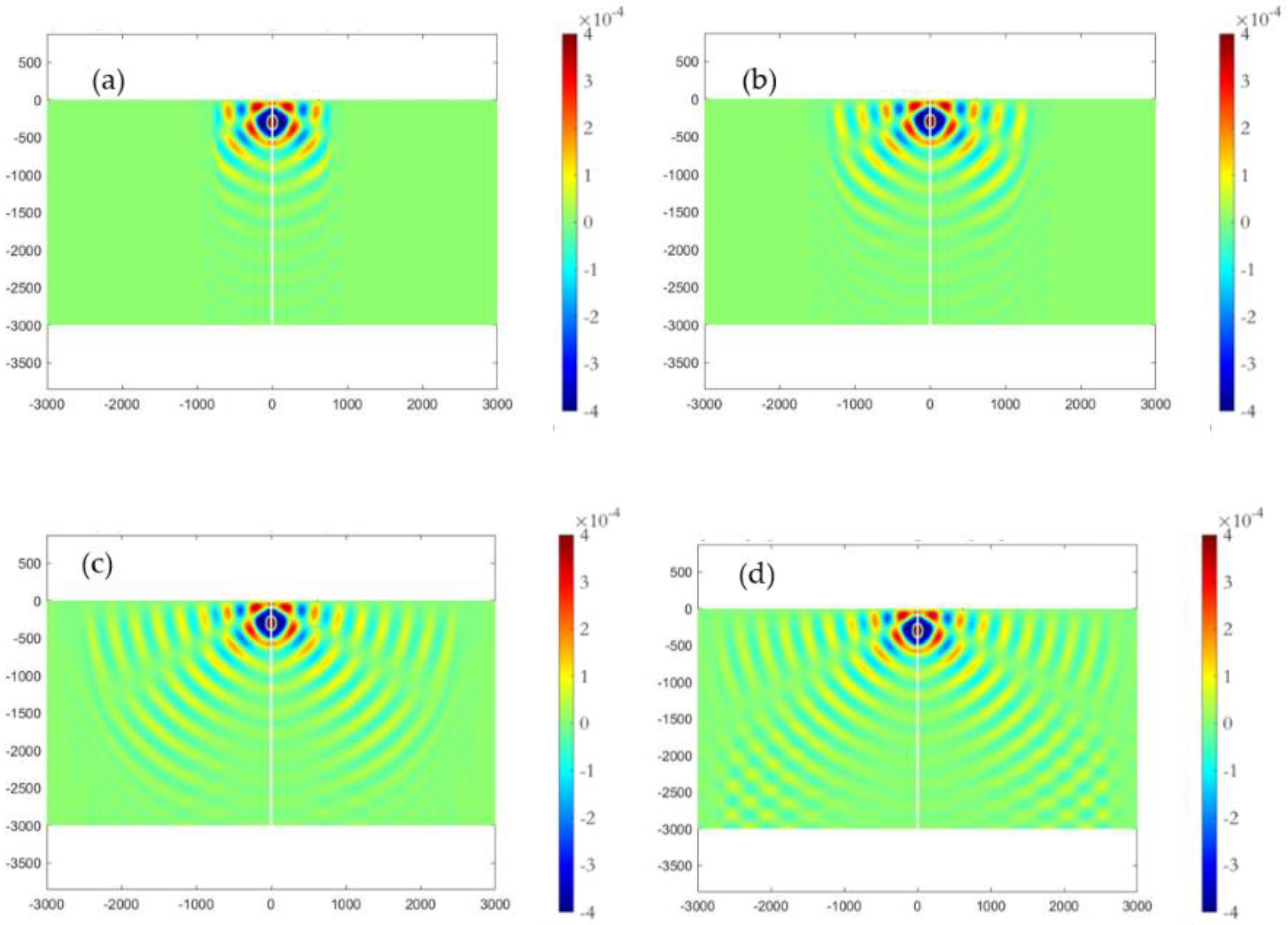
First, a homogenous (isovelocity) environment is considered, with the constant depth set as $h\hspace{0.17em}=\hspace{0.17em}3000\hspace{0.17em}\mathrm{m}$ and the calculated acoustic field excited by monopole, horizontal, and vertical dipole sources of constant intensity is presented in Figure 7, Figure 8, Figure 9 and Figure 10. In order to illustrate the time evolution of the solution, in Figure 7 the acoustic field generated by the monopole source is plotted at time instants after 1, 3, 7, and 14 periods from the beginning of the calculation. 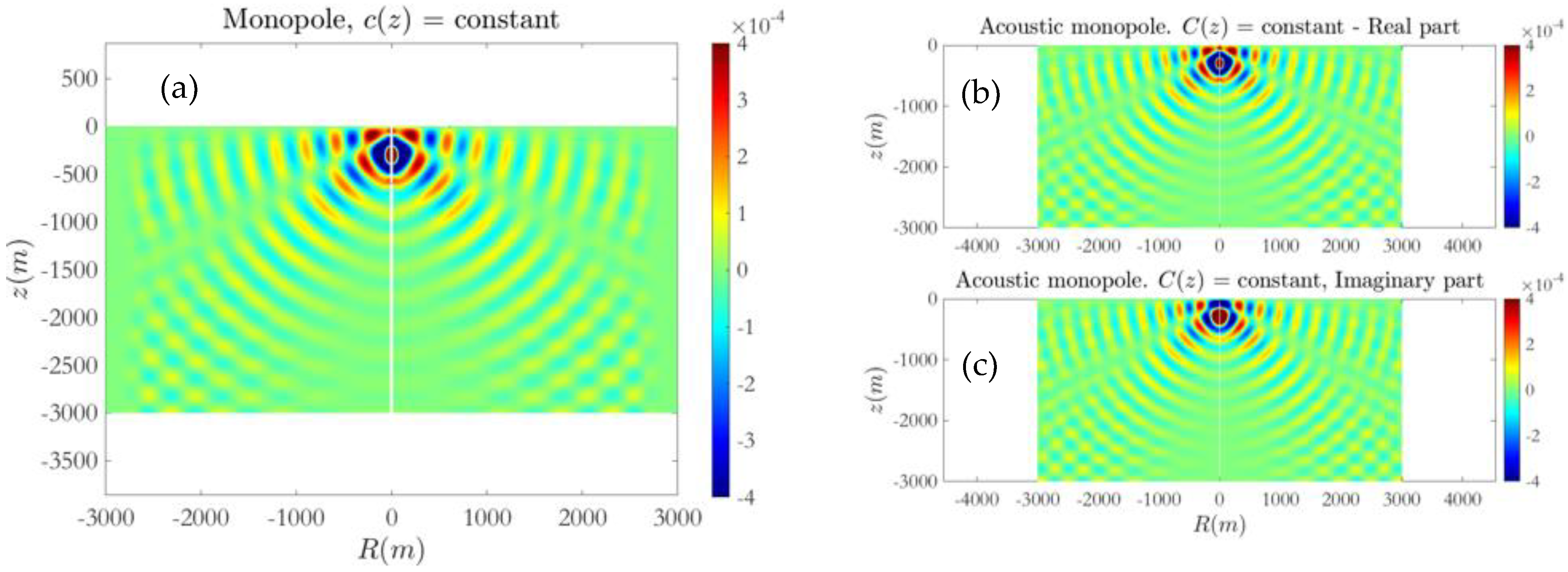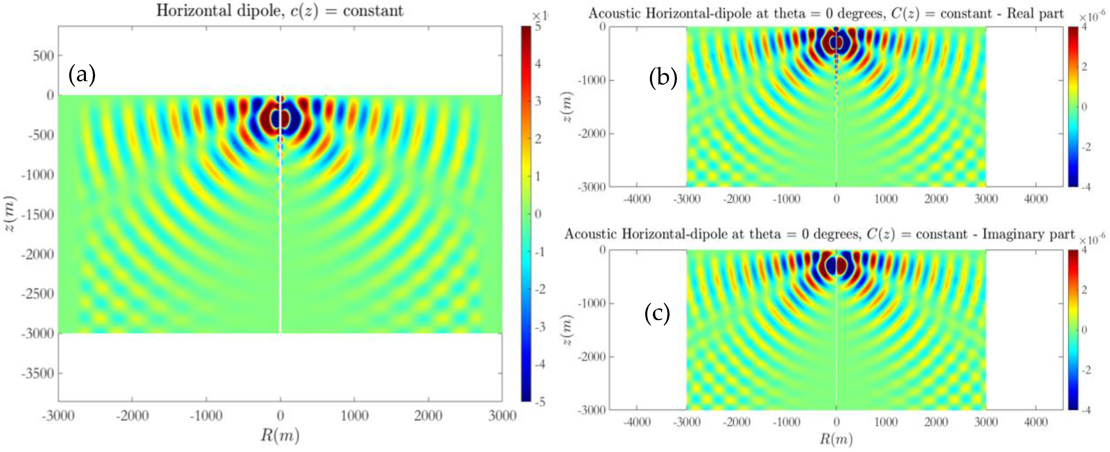Subsequently, in Figure 8, Figure 9 and Figure 10 the periodic results obtained after 15 periods are compared against the solutions of the Helmholtz equation, for the monopole and dipole sources, respectively. In order to avoid numerical dissipation, the horizontal length of the relaxation source field zone is selected in the order of wavelengths. The results presented here and in the sequel correspond to delta-type forcing in the right-hand side of Equation (22), and thus, are normalized with respect to the monopole/dipole source amplitude.

In the case of the isovelocity environment, a comparison of the computed solution using the present FDTD–PML scheme and the Helmholtz equation is presented in Figure 8, Figure 9 and Figure 10. Numerical results concerning the acoustic field excited by the monopole/dipole sources at $f\hspace{0.17em}=\hspace{0.17em}5\hspace{0.17em}\mathrm{Hz}$ are obtained using a $r\hspace{0.17em}-\hspace{0.17em}z$ grid consisting of 300 by 150 points, and Δt = 0.005 s corresponding to 40 time steps in a period, which provides a Courant number of $C\hspace{0.17em}=\hspace{0.17em}c/\left(\Delta x/\Delta t\right)\hspace{0.17em}=\hspace{0.17em}0.75$, that is sufficient for convergence and stability of the present FDTD method.

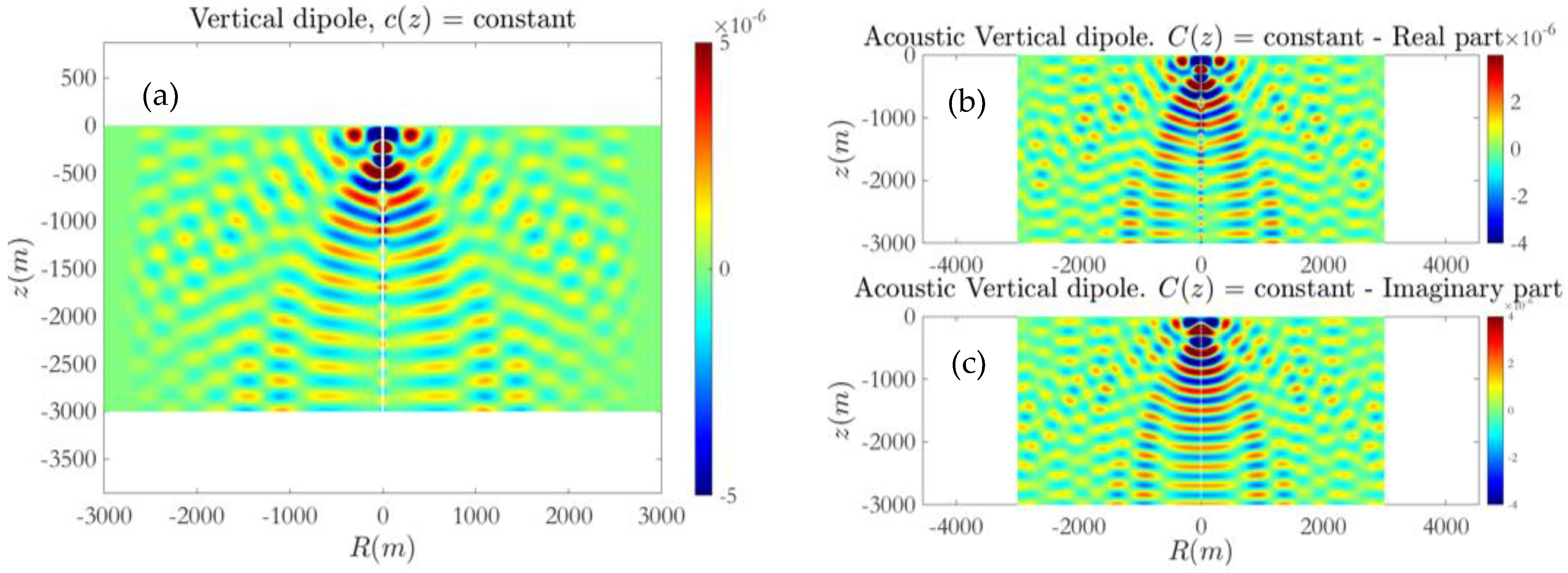
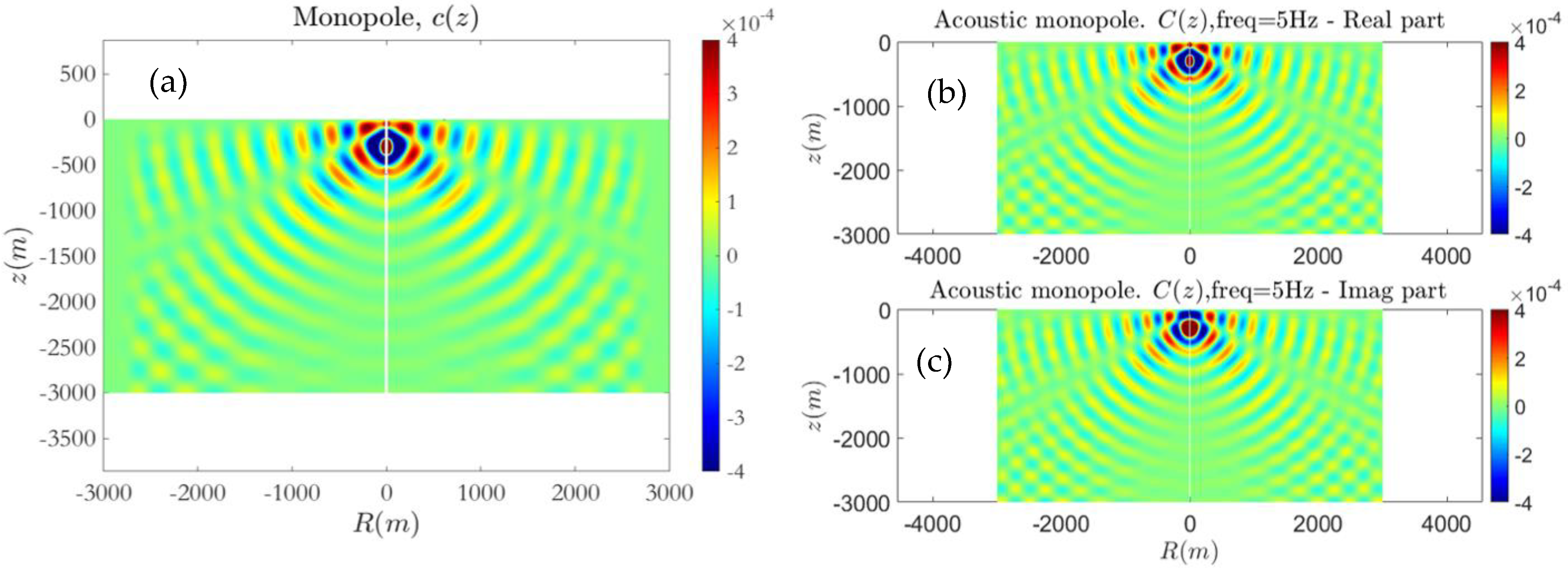
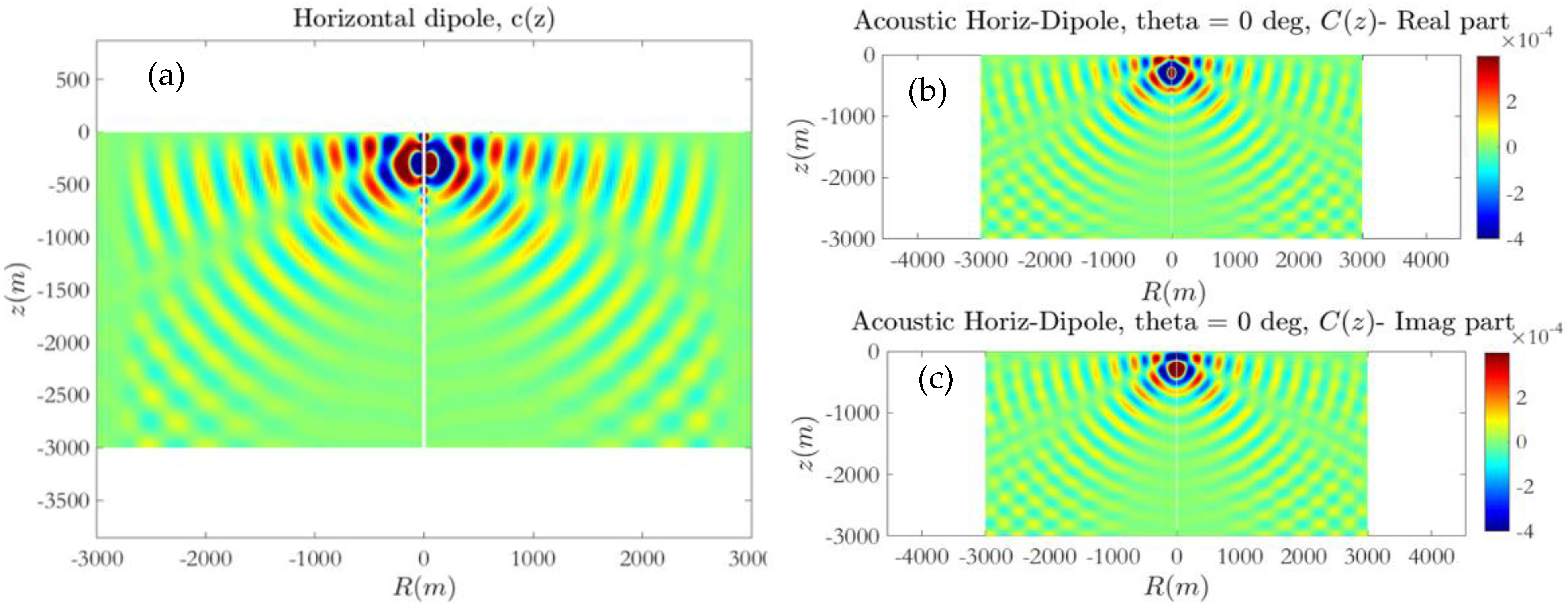
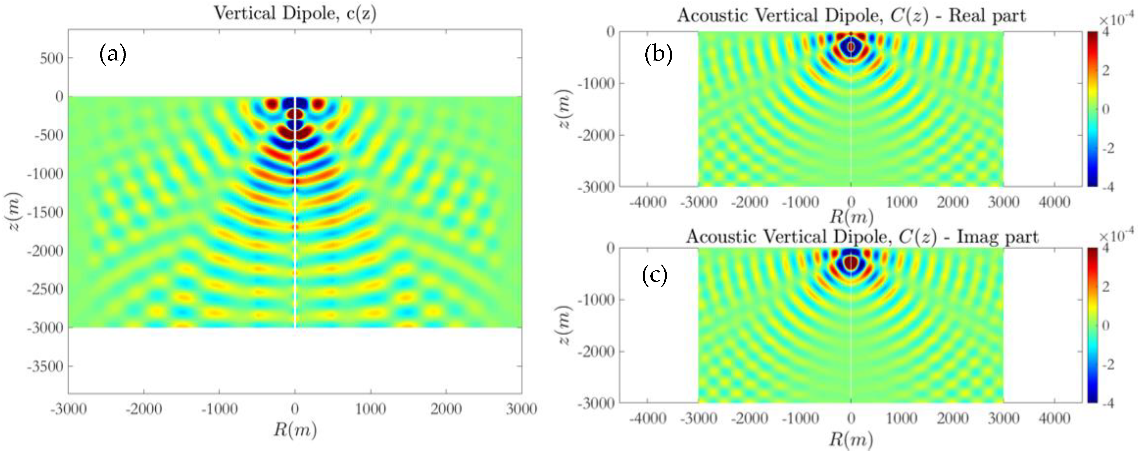
Similar results obtained in the case of underwater acoustic propagation in the sea acoustic waveguide characterized the vertical sound–speed profile, shown in Figure 8, are presented for the monopole, horizontal and vertical dipole source in Figure 11, Figure 12 and Figure 13, respectively, along with comparison with the results from the frequency domain where the VEP is solved with a finite difference scheme. It is seen in the aforementioned figures that the propagation pattern is modified by the presence of additional boundaries and refraction phenomena that manifest at higher frequencies. In particular, the effect of the free surface and hard bottom modifies the noise pattern significantly.

6. Extension to the Case of the Impedance-Type Seabed Model

Next, the present acoustic model is extended in the case of a more realistic sea bottom which is represented as an impedance boundary. In order to quantify the seabed acoustic parameter, the Pekeris waveguide consisting of a homogeneous layer overlying a homogeneous half-space is considered. In the latter two-layer medium, the sound velocity, attenuation, and density can be discontinuous from layer to layer. In this work, we will proceed to the formulation of an impedance-type seabed model using the Pekeris waveguide analysis; see [12]. In this case, an isovelocity water layer lies over an isovelocity half-space bottom and a boundary condition is applied in the interface between the layers. The general solution in the half space is given by:

$$Z_n\hspace{0.17em}=\hspace{0.17em}B{e}^{-{\gamma }_{b}z}\hspace{0.17em}+\hspace{0.17em}C{e}^{{\gamma }_{b}z}$$

(45)

where ${\gamma }_b^2\hspace{0.17em}=\hspace{0.17em}{k}_{rn}^2\hspace{0.17em}-\hspace{0.17em}{\left(\frac{\omega }{c_b}\right)}^2\hspace{0.17em}$ and $c_b$ represent the sound speed in the seabed. Requiring a bounded solution, the above equation reduces to:

$$Z_n\hspace{0.17em}=\hspace{0.17em}B{e}^{-{\gamma }_{b}z}$$

(46)

At the interface between the two layers, we require the continuity of pressure and normal velocity:

$$Z_n\left(D\right)\hspace{0.17em}=\hspace{0.17em}B{e}^{-{\gamma }_{b}z},\hspace{0.17em}\frac{1}{\rho }\frac{d{Z}_n\left(D\right)}{dz}\hspace{0.17em}=\hspace{0.17em}-{\gamma }_b\frac{B{e}^{-{\gamma }_{b}z}}{{\rho }_b}$$

(47)

and from the solution of the corresponding VEP we obtain (see also [12],)

$$f\left(k_{rn}^2\right)Z_n\left(D\right)\hspace{0.17em}+\hspace{0.17em}\frac{g\left(k_{rn}^2\right)}{\rho }\frac{d{Z}_n\left(D\right)}{dz}\hspace{0.17em}=\hspace{0.17em}0$$

(48)

where $f\left(k_{rn}^2\right)\hspace{0.17em}=\hspace{0.17em}1$ and $g\left(k_{rn}^2\right)\hspace{0.17em}=\hspace{0.17em}{\rho }_b/\sqrt{k_{rn}^2\hspace{0.17em}-\hspace{0.17em}{\left(\frac{\omega }{c_b}\right)}^2}$. Thus, the impedance seabed BC is written in the form:

$$\frac{d{Z}_n}{dz}{|}_{z=-h}\hspace{0.17em}+\hspace{0.17em}i\left|A\right|Z_n\left(z\hspace{0.17em}=\hspace{0.17em}-h\right)\hspace{0.17em}=\hspace{0.17em}0$$

(49)

where the modulus of the coefficient $A$ is given by

$$\left|A\right|\hspace{0.17em}=\hspace{0.17em}\frac{\rho }{{\rho }_b}\sqrt{k_{rn}^2\hspace{0.17em}-\hspace{0.17em}{\left(\frac{\omega }{c_b}\right)}^2}$$

(50)

The latter quantity is mode dependent, however, an efficient value is estimated by considering the first mode wavenumbers. From the above equation, we see that the value of $\left|A\right|\hspace{0.17em}$ is small. Using the above results the following Vertical Eigenvalue Problem is formulated in the case of an impedance seabed model:

$$\frac{d^2{Z}_n\left(z\right)}{d{z}^2}\hspace{0.17em}+\hspace{0.17em}\left[\frac{{\omega }^2}{c^2}\hspace{0.17em}-\hspace{0.17em}{\left(k_{zn}^I\right)}^2\right]Z_n\left(z\right)\hspace{0.17em}=\hspace{0.17em}0$$

(51)

with boundary conditions:

$$Z_n\left(z\hspace{0.17em}=\hspace{0.17em}0\right)\hspace{0.17em}=\hspace{0.17em}0,\hspace{0.17em}\hspace{0.17em}\hspace{0.17em}\hspace{0.17em}\hspace{0.17em}\frac{d{Z}_n}{dz}{|}_{z=-h}\hspace{0.17em}+\hspace{0.17em}A{Z}_n\left(z\hspace{0.17em}=\hspace{0.17em}-h\right)\hspace{0.17em}=\hspace{0.17em}0$$

(52)

where the superscript $I$ denotes the eigenvalues of impedance-type sea bottom BC VEP.

The general solution is:

$$Z_n\left(z\right)\hspace{0.17em}=\hspace{0.17em}{A}_n\cos \left({\lambda }_{n}z\right)\hspace{0.17em}+\hspace{0.17em}{B}_n\sin \left({\lambda }_{n}z\right), \mathrm{where} {\lambda }_n\hspace{0.17em}=\hspace{0.17em}{k}^2\hspace{0.17em}-\hspace{0.17em}{\left(k_{zn}^I\right)}^2,$$

(53)

and by applying the boundary conditions on the free surface and the impedance bottom we obtain the following eigenvalue equation:

$$\frac{k_{zn}^{I}h}{Ah}\hspace{0.17em}=\hspace{0.17em}\tan \left(k_{zn}^{I}h\right),\hspace{0.17em}\mathrm{where}\hspace{0.17em}A=i\left|A\right|,$$

(54)

which is put into a nondimensional form as follows

$$\hspace{0.17em}{z}_n\cos z_n\hspace{0.17em}-\hspace{0.17em}i\widehat{A}\sin z_n\hspace{0.17em}=\hspace{0.17em}0,\hspace{0.17em}\mathrm{where}\hspace{0.17em}{z}_n=k_{zn}^{I}h,\hspace{0.17em}\mathrm{and}\hspace{0.17em}\widehat{A}=Ah$$

(55)

Clearly, the case $A\hspace{0.17em}=\hspace{0.17em}0$ corresponds to a hard bottom (Neumann) boundary condition

$$k_{zn}^N\hspace{0.17em}=\hspace{0.17em}\frac{\left(n\hspace{0.17em}-\hspace{0.17em}0.5\right)\pi }{h},\hspace{0.17em}n=1,2,\dots ,$$

(56)

and for $A\hspace{0.17em}\to \hspace{0.17em}\infty$ we have a soft (Dirichlet) boundary condition:

$$k_{zn}^D\hspace{0.17em}=\hspace{0.17em}\left(n\hspace{0.17em}-\hspace{0.17em}1\right)\pi ,\hspace{0.17em}n=1,2,\dots \hspace{0.17em}.$$

(57)

For small values of $\left|A\right|\hspace{0.17em}$, an asymptotic analysis is possible providing a very good approximation as presented in the sequel. Allowing $z_n\hspace{0.17em}=\hspace{0.17em}{r}_n\hspace{0.17em}+\hspace{0.17em}i{\epsilon }_n$, where $r_n\hspace{0.17em}=\hspace{0.17em}\left(n\hspace{0.17em}-\hspace{0.17em}0.5\right)\pi$ is the Neumann eigenvalues, and substituting into Equation (55), we obtain:

$$z_n\hspace{0.17em}=\hspace{0.17em}\left(n\hspace{0.17em}-\hspace{0.17em}0.5\right)\pi \hspace{0.17em}-\hspace{0.17em}\frac{i\widehat{A}}{\left(n\hspace{0.17em}-\hspace{0.17em}0.5\right)\pi } \mathrm{for} n\hspace{0.17em}=\hspace{0.17em}1,2,\mathrm{\dots }$$

(58)

and the seabed impedance eigenvalues are approximated by:

$$k_{zn}^{I}h\hspace{0.17em}=\hspace{0.17em}\hspace{0.17em}\left(n\hspace{0.17em}-\hspace{0.17em}0.5\right)\pi \hspace{0.17em}-\hspace{0.17em}\frac{i\widehat{A}}{\left(n\hspace{0.17em}-\hspace{0.17em}0.5\right)\pi }\hspace{0.17em} \mathrm{for} n\hspace{0.17em}=\hspace{0.17em}1,2,\mathrm{\dots }$$

(59)

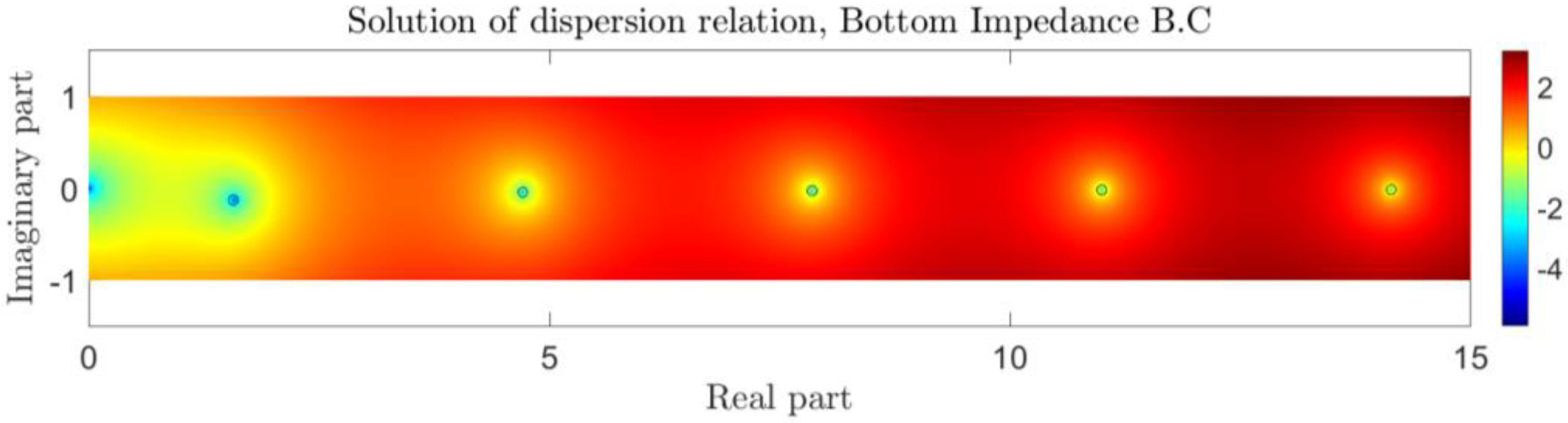
As an example, in the case of $\widehat{A}=0.001$ and h = 3000 m, c = 1500 m/s, the solution of the eigenvalue Equation (55) on the complex plane is shown in Figure 14, where the approximation provided by Equation (59) is also plotted using circles, and we observe that it provides excellent predictions.

Based on the above Green’s function of the Helmholtz equation, in the case of an ocean acoustic waveguide with impedance seabed BC is expressed as follows:

$$G_I\hspace{0.17em}=\hspace{0.17em}\frac{i}{4h}{\displaystyle \sum _{n\hspace{0.17em}=\hspace{0.17em}1}^{\infty }\sin \left(k_{zn}^{I}z\right)}\sin \left(k_{zn}^I{z}_s\right)H_0^{\left(1\right)}\left(k_n^{I}r\right),\hspace{0.17em}\hspace{0.17em}\hspace{0.17em}{k}_n^I={\left[\frac{{\omega }^2}{c^2}\hspace{0.17em}-\hspace{0.17em}{\left(k_{zn}^I\right)}^2\right]}^{1/2}$$

(60)

Thus, after deriving the eigenvalues $k_{zn}^I$, the above analytical expression obtained using the normal-mode expression of the Green’s function and its derivatives in the $x_s,z_s$ direction of the location of the source could be similarly exploited to model the monopole, horizontal, and vertical dipole sources, respectively, over an impedance seabed boundary. These expressions will be used to enforce near-source field data by applying, again, a relaxation scheme, as already discussed in Section 4.2.

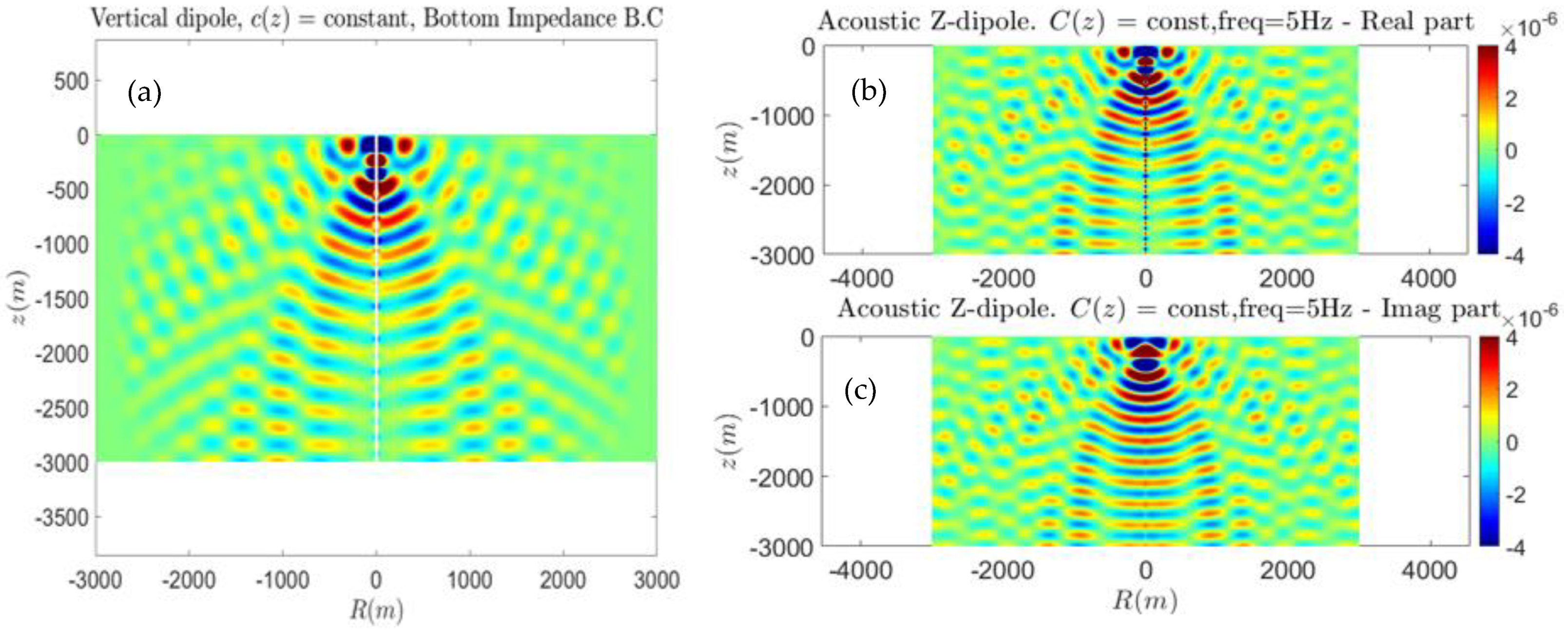
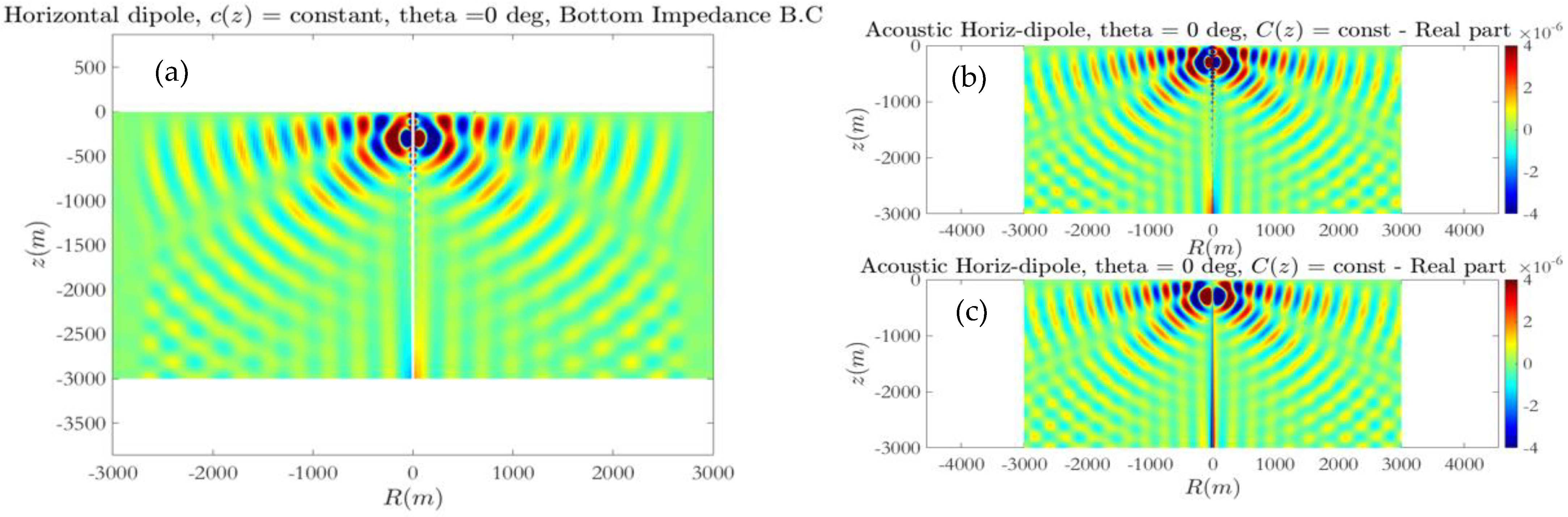
Next, the numerical results obtained using the present FDTD–PML numerical scheme for the case of an impedance-type BC for the modeling of the seabed effects in the acoustic propagation are presented for the monopole, horizontal and vertical dipole source in Figure 15, Figure 16 and Figure 17, respectively, and compared and verified with results from the solution of the Helmholtz equation. The effect of the bottom scattering field is clearly observed in contrast with the hard bottom case.

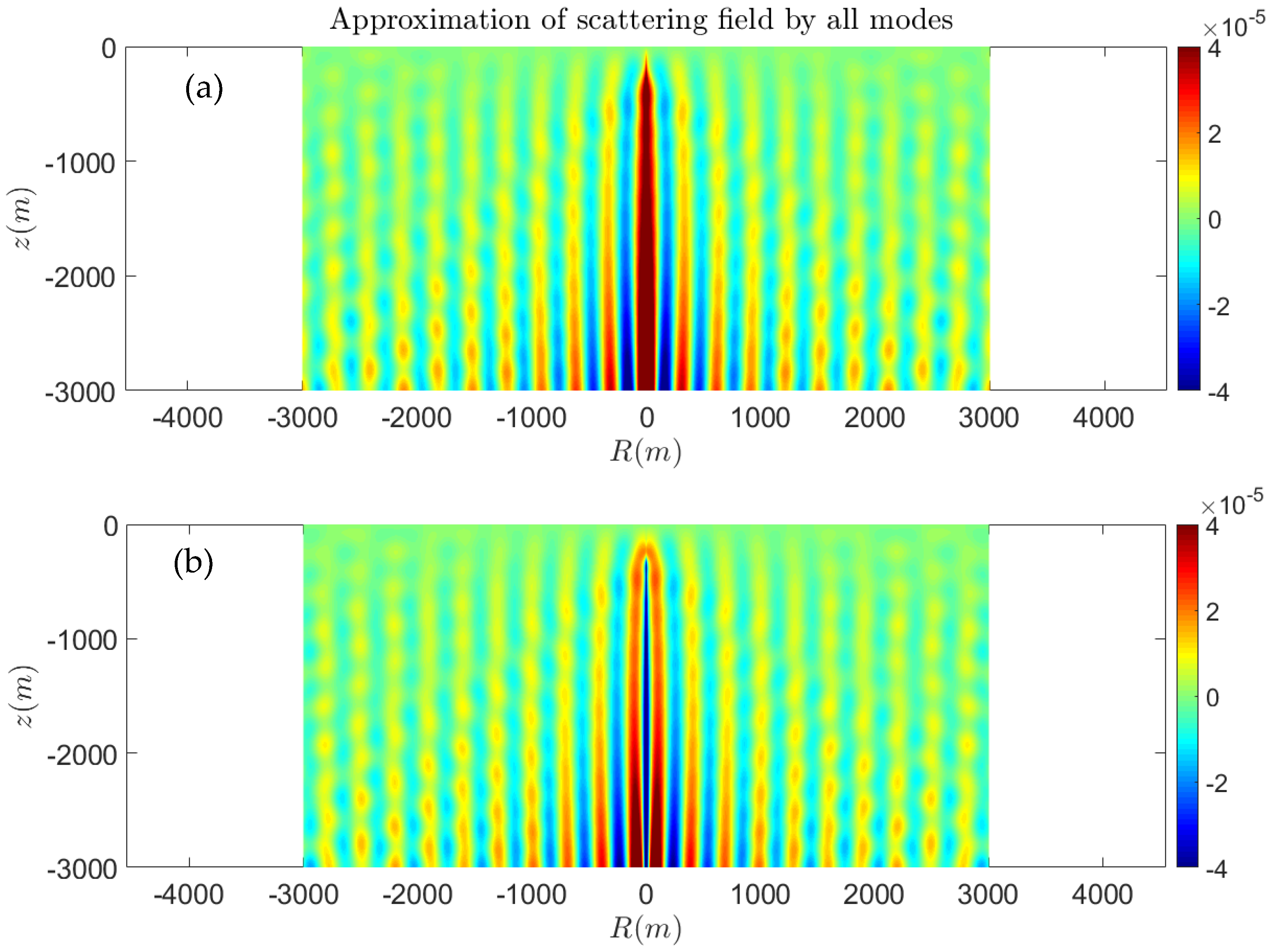
Finally, having obtained normal mode expressions of the Green’s function for the impedance sea bottom $G_I\hspace{0.17em}$ and for the hard seabed $G_N\hspace{0.17em}$, respectively, the results can be used to derive an alternative representation of the impedance sea bottom singularity in the form: $G_I\hspace{0.17em}=G_N\hspace{0.17em}+ \hspace{0.17em}{p}_{scat}$, where $p_{scat}$ is a regular scattering field excited by the sea bottom data.

As an example, the scattering field is presented in Figure 18 as obtained using $\hspace{0.17em}{p}_{scat}\hspace{0.17em}=G_I\hspace{0.17em}-\hspace{0.17em}{G}_N\hspace{0.17em}$ in the case of a monopole source located at z₀ = −300 m and with parameters $\widehat{A}=0.001$, h = 3000 m, and $c\hspace{0.17em}=\hspace{0.17em}1500$ m/s. Comparing this result with Figure 11, we observe that the scattering field due to the effect of the impedance seabed is an order of magnitude less than the source field and is maximized on the sea bottom.

The above alternative representation will be exploited in future work for formulating and solving scattering problems in the inhomogeneous ocean waveguide characterized by an impedance seabed with the additional presence of obstacles modeling the effects of ocean vehicles or AUVs modifying the directivity pattern of the acoustic field generated by the monopole and dipole sources associated with the hydrodynamic flapping thruster loads. For this purpose, appropriate 3D BEM methods have been developed; see, e.g., [53].

7. Conclusions

The effects of noise generation and propagation by flapping thrusters used for small ships and AUV propulsion were studied. A new and efficient, low-cost numerical method based on finite differences and absorbing layer techniques was presented and validated for treating noise propagation in large domains and lengthy time simulations. The present FDTD–PML numerical scheme extends the standard acoustic model from free space to the inhomogeneous ocean waveguide in a 3D cylindrical environment including free-surface and bottom-boundary effects, as well as refraction/diffraction phenomena due to sound–speed variations. For simplicity, the axisymmetric sea acoustic waveguide was considered. A Perfectly Matched Layer technique was employed for the treatment of the outgoing radiating field behavior in the open boundaries. For the verification of the present method, the numerical results in the case of fields excited by monopole and dipole sources were presented with a comparison against a frequency domain solution both for an isovelocity environment and variable sound-speed profile in the case of a hard seabed boundary. The acoustic model is further extended by employing an impedance-type seabed model, allowing for a more realistic approach of the sea bottom. The FDTD–PML numerical scheme is in good agreement in comparison with analytical solutions and exhibits low computational cost, which makes it appropriate for large domains and lengthy time simulations. Future work will be directed towards the modeling of more complex range-dependent waveguide configurations, as in the case of variable seabed profiles using a curvilinear FDTD–PML scheme on a structured grid derived using conformal mapping and differential system techniques. The Green’s function for an impedance-type seabed will used for the implementation of 3D BEM treating noise propagation by flapping propulsors of ocean and underwater vehicles, providing useful information concerning the directivity pattern of the acoustic field generated by the hydrodynamic flapping thruster loads.

References

1. McKenna, M.F.; Ross, D.; Wiggins, S.M.; Hildebrand, J.A. Underwater radiated noise from modern commercial ships. J. Acoust. Soc. Am. 2012, 131, 92–103. [Google Scholar] [CrossRef] [PubMed]
2. United Nations Conference on Trade and Development [UNCTAD]. Review of Maritime Transport 2018; No. 9211128412; United Nations Conference on Trade and Development: Geneva, Switzerland, 2018. [Google Scholar]
3. IMO 2014. Guidelines for the Reduction of Under-Water Noise from Commercial Shipping to Address Adverse Impacts on Marine Life—Non Mandatory Technical Advices; International Maritime Organization: London, UK, 2014. [Google Scholar]
4. Ross, D. Mechanics of Underwater Noise; Pergamon Press: New York, NY, USA, 1976. [Google Scholar]
5. Belibassakis, K.A.; Politis, G.K. Hydrodynamic performance of flapping wings for augmenting ship propulsion in waves. Ocean Eng. 2013, 72, 227–240. [Google Scholar] [CrossRef]
6. Belibassakis, K.A.; Filippas, E.S. Ship propulsion in waves by actively controlled flapping foils. Appl. Ocean Res. 2015, 52, 1–11. [Google Scholar] [CrossRef]
7. Wu, X.; Zhang, X.; Tian, X.; Li, X.; Lu, W. A review on fluid dynamics of flapping foils. Ocean Eng. 2020, 195, 106712. [Google Scholar] [CrossRef]
8. Duarte, C.M.; Chapuis, L.; Collin, S.P.; Costa, D.P.; Devassy, R.P.; Eguiluz, V.M.; Erbe, C.; Gordon, T.A.C.; Halpern, B.S.; Harding, H.R.; et al. The soundscape of the Anthropocene ocean. Science 2021, 371, 6529. [Google Scholar] [CrossRef]
9. Belibassakis, K.A.; Politis, G. Generation and Propagation of Noise from Cavitating Marine Propellers, 6th ed.; Symposium on Marine Propulsors smp: Rome, Italy, 2019. [Google Scholar]
10. Sun, X.; Wang, X. Fundamentals of Aeroacoustics with Applications to Aeropropulsion Systems; Elsevier: San Diego, CA, USA, 2020. [Google Scholar]
11. Athanassoulis, G.A.; Belibassakis, K.A.; Mitsoudis, D.A.; Kampanis, D.A.; Dougalis, V.A. Coupled mode and finite element approximations of underwater sound propagation problems in general stratified en-vironments. J. Comput. Acoust. 2008, 16, 83–116. [Google Scholar] [CrossRef]
12. Jensen, F.; Kuperman, W.; Porter, M.; Schmidt, H. Computational Ocean Acoustics, 2nd ed.; Springer: Berlin/Heidelberg, Germany, 2011. [Google Scholar]
13. Petris, G.; Cianferra, M.; Armenio, V. A numerical method for the solution of the three-dimensional acoustic wave equation in a marine environment considering complex sources. Ocean Eng. 2022, 256, 111459. [Google Scholar] [CrossRef]
14. Triantafyllou, M.S.; Triantafyllou, G.S.; Yue, D.K.P. Hydrodynamics of fishlike swimming. Annu. Rev. Fluid Mech. 2000, 32, 33–53. [Google Scholar] [CrossRef]
15. Triantafyllou, M.S.; Techet, A.H.; Hover, F.S. Review of experimental work in biomimetic foil. IEEE J. Ocean. Eng. 2004, 29, 585–594. [Google Scholar] [CrossRef]
16. von Ellenrieder, K.D.; Parker, K.; Soria, J. Fluid mechanics of flapping wing. Exp. Therm. Fluid Sci. 2008, 32, 1578–1589. [Google Scholar] [CrossRef]
17. Taylor, G.; Triantafyllou, M.S.; Tropea, C. (Eds.) Animal Locomotion; Springer: Berlin/Heidelberg, Germany, 2010; pp. 1–443. [Google Scholar]
18. Ci, X.; Fan, S.; Jin, Y. Design and Operation Optimization of the Flapping Fin for AUV Propulsion. In 2019 IEEE Underwater Technology (UT); IEEE: Piscataway, NJ, USA, 2019; pp. 1–9. [Google Scholar]
19. Filippas, E.; Papadakis, G.; Belibassakis, K.A. Free-Surface Effects on the Performance of Flapping-Foil Thruster for Augmenting Ship Propulsion in Waves. J. Mar. Sci. Eng. 2020, 8, 357. [Google Scholar] [CrossRef]
20. Belibassakis, K.; Filippas, E.; Papadakis, G. Numerical and Experimental Investigation of the Performance of Dynamic Wing for Augmenting Ship Propulsion in Head and Quartering Seas. J. Mar. Sci. Eng. 2021, 10, 24. [Google Scholar] [CrossRef]
21. Katz, J.; Plotkin, A. Low-Speed Aerodynamics; Cambridge University Press: Cambridge, UK, 1990; Volume 13. [Google Scholar]
22. Filippas, E.; Belibassakis, K.A. Hydrodynamic analysis of flapping-foil thrusters operating beneath the free surface and in waves. Eng. Anal. Bound. Elem. 2014, 41, 47–59. [Google Scholar] [CrossRef]
23. Filippas, E.S.; Belibassakis, K.A. A nonlinear time-domain BEM for the performance of 3D flapping-wing thrusters in directional waves. Ocean Eng. 2022, 245, 110157. [Google Scholar] [CrossRef]
24. Politis, G.; Tsarsitalidis, V. Flapping wing propulsor design: An approach based on systematic 3D-BEM simulations. Ocean Eng. 2014, 84, 98–123. [Google Scholar] [CrossRef]
25. Schouveiler, L.; Hover, F.S.; Triantafyllou, M.S. Performance of flapping foil propulsion. J. Fluids Struct. 2005, 20, 949–959. [Google Scholar] [CrossRef]
26. Belibassakis, K.; Malefaki, I. Noise Generation and Propagation by Biomimetic Dynamic-Foil Thruster. In Proceedings of the Euronoise, Madeira, Portugal, 25–27 October 2021. [Google Scholar]
27. Lighthill, M.J. On sound generated aerodynamically. I. General theory. Proc. R. Soc. Lond. Ser. A. Math. Phys. Sci. 1952, 211, 564–587. [Google Scholar]
28. Ffowcs Williams, J.E.; Hawkings, D.L. Sound Generated by Turbulence and Surfaces in Arbitrary Motion. Philos. Trans. R. Soc. 1969, 264, 321–342. [Google Scholar]
29. Brentner, K.S. Modeling Aerodynamically Generated Sound: Recent Advances in Rotor Noise Prediction. In Proceedings of the 38th Aerospace Sciences Meeting and Exhibit, Reno, NV, USA, 10–13 January 2000. [Google Scholar]
30. Ianniello, S.; Muscari, R.; Mascio, A. Ship underwater noise assessment by the acoustic analogy. Part I: Nonlinear analysis of a marine propeller in a uniform flow. J. Mar. Sci. Technol. 2013, 18, 547–570. [Google Scholar] [CrossRef]
31. Ianniello, S.; Muscari, R.; Di Mascio, A. Ship underwater noise assessment by the Acoustic Analogy. Part II: Hydroacoustic analysis of a ship scaled model. J. Mar. Sci. Technol. 2014, 19, 52–74. [Google Scholar] [CrossRef]
32. Ianniello, S.; De Bernardis, E. Farassat’s formulations in marine propeller hydroacoustics. Int. J. Aeroacoustics 2015, 14, 87–103. [Google Scholar] [CrossRef]
33. Testa, C.; Porcacchia, F.; Zaghi, S.; Gennaretti, M. Study of a FWH-based permeable-surface formulation for propeller Hydroacoustics. Ocean Eng. 2021, 240, 109828. [Google Scholar] [CrossRef]
34. Belibassakis, K. A velocity-based BEM for modeling generation and propagation of underwater noise from marine propellers. In Proceedings of the Euronoise, Crete, Greece, 27–31 May 2018. [Google Scholar]
35. Farassat, F. Acoustic radiation from rotating blades—The Kirchhoff method in aeroacousics. J. Sound Vib. 2001, 239, 785–800. [Google Scholar] [CrossRef]
36. Farassat, F.; Myers, M.K. Aerodynamics via Acoustics: Application of Acoustic Formulas for Aerodynamic Calculations. In Proceedings of the 10th Aeroacoustics Conference, Seattle, WA, USA, 9–11 July 1986; pp. 86–1877. [Google Scholar]
37. Seol, H.; Suh, J.C.; Lee, S. Development of hybrid method for the prediction of underwater propeller noise. J. Sound Vib. 2005, 288, 345–360. [Google Scholar] [CrossRef]
38. Brekhovskikh, L.M.; Godin, O.A. Acoustics of Layered Media; Springer: Berlin/Heidelberg, Germany, 1990. [Google Scholar]
39. Givoli, D. Numerical Methods for Problems in Infinite Domains; Elsevier: Amsterdam, The Netherlands, 1992. [Google Scholar]
40. Bérenger, J.-P. A perfectly matched layer for the absorption of electromagnetic waves. J. Comput. Phys. 1994, 114, 185–200. [Google Scholar] [CrossRef]
41. Appelö, D.; Hagstrom, T.; Kreiss, G. Perfectly matched layers for hyperbolic systems: General formulation, well-posedness, and stability. SIAM J. Appl. Math. 2006, 67, 1–23. [Google Scholar] [CrossRef]
42. Zhao, L.; Cangellaris, A. A general approach for the development of unsplit-field time-domain implementations for perfectly matched layers for FDTD grid truncation. IEEE Microw. Guided Wave Lett. 1996, 6, 209–211. [Google Scholar] [CrossRef]
43. Lähivaara, T.; Huttunen, T. A non-uniform basis order for the discontinuous Galerkin method of the 3D dissipative wave equation with perfectly matched layer. J. Comput. Phys. 2010, 229, 5144–5160. [Google Scholar] [CrossRef]
44. Hu, F.Q. A stable, perfectly matched layer for linearized Euler equations in unsplit physical variables. J. Comput. Phys. 2001, 173, 455–480. [Google Scholar] [CrossRef]
45. Cohen, G.C. Higher-Order Numerical Methods for Transient Wave Equations; Springer: Berlin/Heidelberg, Germany, 2002. [Google Scholar]
46. Grote, M.; Sim, I. Efficient PML for the wave equation. arXiv 2010, arXiv:1001.0319. [Google Scholar]
47. Diaz, J.; Joly, P. A time domain analysis of PML models in acoustics. Comput. Methods Appl. Mech. Eng. 2006, 195, 3820–3853. [Google Scholar] [CrossRef]
48. Bermúdez, A.; Hervella-Nieto, L.; Prieto, A.; Rodrı, R. An optimal perfectly matched layer with unbounded absorbing function for time-harmonic acoustic scattering problems. J. Comput. Phys. 2007, 223, 469–488. [Google Scholar] [CrossRef]
49. Karperaki, A.; Papathanasiou, T.K.; Belibassakis, K.A. An optimized, parameter-free PML-FEM for wave scattering problems in the ocean and coastal environment. Ocean Eng. 2019, 179, 307–324. [Google Scholar] [CrossRef]
50. Bécache, E.; Dhia, A.B.B.; Legendre, G. Perfectly matched layers for the time-harmonic acoustics in the presence of uniform flow. SIAM J. Numer. Anal. 2006, 44, 1191–1217. [Google Scholar] [CrossRef]
51. Collino, F.; Monk, P. Optimizing the perfectly matched layer. Comput. Methods Appl. Mech. Eng. 1998, 164, 157–171. [Google Scholar] [CrossRef]
52. Modave, A.; Delhez, E.; Geuzaine, C. Optimizing perfectly matched layers in discrete contexts. Int. J. Numer. Methods Eng. 2014, 99, 410–437. [Google Scholar] [CrossRef]
53. Belibassakis, K.; Prospathopoulos, J.; Malefaki, I. Scattering and directionality effects of noise generation from flapping thrusters used for propulsion of small ocean vehicles. J. Mar. Sci. Eng. 2022, 10, 1129. [Google Scholar] [CrossRef]
Figure 1. Flapping thruster: consecutive positions of foil oscillatory motion and trailing vortex wake associated with the formation of a reverse Karman vortex street leading to the generation of oscillatory vertical lift force and horizontal thrust force (red arrows) with a significant non-zero mean (blue arrow).
Jmse 10 01240 g001
Figure 2. Flapping thruster performance as obtained from the unsteady hydrofoil theory and a comparison with experimental data by [26], in the case of foil of c = 0.1 m , A R = 6 , for U = 0.4 m / s ,   S t r = 2 f h 0 / U = 0.23 , h 0 / c c h o r d = 0.75 , and θ 0 = 23 ° . Time history of the (a) dynamic angle of attack and (b) flapping thruster loads against non-dimensional time t/T, where T = 1/f: C Z = F Z / ( 0.5 ρ U 2 A ) shown by black and red lines and experimental data shown by using circles, and C X = F X / ( 0.5 ρ U 2 A ) shown using cyan lines and experimental data shown using crosses.
Jmse 10 01240 g002
Figure 3. Calculated acoustic field in free space as generated by the flapping thruster operating in water (c = 1500 m/s), in the case of foil of Figure 2 of A R = 6 , flapping at S t r = 0.23 , h 0 / c = 0.75 , and θ 0 = 23 deg , using the hydrodynamic loads in the present method. Total acoustic field in the vicinity of the flapping thruster, normalized with respect to its value at the distance of 1 m from the source, at two instances: (a) when the nose of the flapping thruster is directed upwards. (b) when the nose of the foil is directed downwards.
Jmse 10 01240 g003
Figure 4. A point source in a cylindrical domain.
Jmse 10 01240 g004
Figure 5. Decomposition of the original domain into two non-overlapping subdomains Ω and D .
Jmse 10 01240 g005
Figure 6. Sound speed profiles.
Jmse 10 01240 g006
Figure 7. The acoustic field in the case of the isovelocity c = 1500 m/s environment, obtained using the present FDTD–PML numerical scheme, excited by a monopole source of frequency f = 5   Hz located at a depth of 300 m, after times of (a) 1 period, (b) 3 periods, (c) 7 periods, and (d) 14 periods from the beginning of the calculation.
Jmse 10 01240 g007
Figure 8. (a) The calculated acoustic field for the isovelocity environment, obtained using the present FDTD–PML numerical scheme, excited by a monopole source of frequency f = 5   Hz located at a depth of 300 m, at the end of the computation time after 15 periods. (b,c) Real and imaginary parts of the acoustic field obtained using the solution of the Helmholtz equation excited by a monopole source of frequency f = 5   Hz located at a depth of 300 m.
Jmse 10 01240 g008
Figure 9. (a) The calculated acoustic field for the isovelocity environment, obtained using the present FDTD–PML numerical scheme, excited by a horizontal dipole source of frequency f = 5   Hz located at a depth of 300 m, at the end of the computation time after 15 periods. (b,c) Real and imaginary parts of the acoustic field obtained using the solution of the Helmholtz equation excited by a horizontal dipole source of frequency f = 5   Hz located at a depth of 300 m.
Jmse 10 01240 g009
Figure 10. (a) The calculated acoustic field for the isovelocity environment, obtained using the present FDTD–PML numerical scheme, excited by a vertical dipole source of frequency f = 5   Hz located at a depth of 300 m, at the end of the computation time after 15 periods. (b,c) Real and imaginary parts of the acoustic field solution of the Helmholtz equation excited by a vertical dipole source of frequency f = 5   Hz located at a depth of 300 m.
Jmse 10 01240 g010
Figure 11. (a) The acoustic field obtained using the solution of the FDTD–PML numerical scheme excited by a monopole source of frequency f = 5   Hz located at a depth of 300 m, in the case of a vertically stratified environment. (b,c) Real and imaginary parts of the acoustic field solution of the Helmholtz equation excited by a monopole source of frequency f = 5   Hz located at a depth of 300 m in the stratified velocity environment.
Jmse 10 01240 g011
Figure 12. (a) The acoustic field obtained using the solution of the FDTD–PML numerical scheme excited by a horizontal dipole source of frequency f = 5   Hz located at a depth of 300 m, in the case of a vertically stratified environment. (b,c) Real and imaginary parts of the acoustic field obtained using a solution of the Helmholtz equation excited by a horizontal dipole source of frequency f = 5   Hz located at a depth of 300 m in the stratified velocity environment.
Jmse 10 01240 g012
Figure 13. (a) The acoustic field obtained using the solution of the FDTD–PML numerical scheme excited by a vertical dipole source of frequency f = 5   Hz located at a depth of 300 m in the case of a vertically stratified environment. (b,c) Real and imaginary parts of the acoustic field in the same environment as obtained using the solution of the Helmholtz equation excited by a vertical dipole source of frequency f = 5 Hz located at a depth of 300 m.
Jmse 10 01240 g013
Figure 14. The solution of the eigenvalue Equation (55) in the isovelocity case and small values of the impedance parameter A ^ = 0.001 on the complex plane, and the comparison of the exact and approximate solutions given by Equation (59) shown using black circles.
Jmse 10 01240 g014
Figure 15. (a) The acoustic field obtained using the solution of the FDTD–PML numerical scheme excited by a monopole source of frequency f = 5   Hz located at a depth of 300 m with an impedance bottom boundary condition in the isovelocity environment. (b,c) Real and imaginary parts of the acoustic field obtained using the solution of the Helmholtz equation excited by a monopole source of frequency f = 5   Hz located at a depth of 300 m with an impedance boundary condition.
Jmse 10 01240 g015
Figure 16. (a) The acoustic field obtained using the solution of the FDTD–PML numerical scheme excited by a horizontal dipole source of frequency f = 5   Hz located at a depth of 300 m with an impedance bottom boundary condition in an isovelocity environment. (b,c) Real and imaginary parts of the acoustic field obtained using the solution of the Helmholtz equation excited by a horizontal dipole source of frequency f = 5   Hz located at a depth of 300 m with an impedance boundary condition.
Jmse 10 01240 g016
Figure 17. (a) The acoustic field obtained using the solution of the FDTD–PML numerical scheme excited by a vertical dipole source of frequency f = 5   Hz located at a depth of 300 m with an impedance bottom boundary condition in an isovelocity environment. (b,c) Real and imaginary parts of the acoustic field obtained using the solution of the Helmholtz equation excited by a vertical dipole source of frequency f = 5   Hz located at a depth of 300 m with an impedance boundary condition.
Jmse 10 01240 g017
Figure 18. (a) Real and (b) imaginary parts of the scattering field p s c a t = G I G N .
Jmse 10 01240 g018
Publisher’s Note: MDPI stays neutral with regard to jurisdictional claims in published maps and institutional affiliations.