Numerical Research of the Pressure Fluctuation of the Bow of the Submarine at Different Velocities

Abstract

A numerical analysis based on stress-blended eddy simulation was conducted to investigate the pressure fluctuation of the bow of a submarine at various velocities (5.93 kn, 10 kn, and 12 kn). The simulation results were compared with the experimental data to demonstrate the validity of the numerical method. Self-power spectrum and wave-number frequency spectrum were discussed from the perspective of energy. The results show that with increasing submarine velocity, the pressure fluctuation in the axial direction increases, the transition point moves forward, and the frequency of the Tollmien–Schlichting wave raises.

1. Introduction

Turbulent wall pressure fluctuation is an important hydrodynamic noise source, and it is necessary to carry out the corresponding calculation and experimental research. In addition, the sonar is installed on the bow of the submarine, and it is easily affected by self-noise. Therefore, it is important to understand the change in the flow field on the bow at different velocities to improve the performance of the submarine itself.

Benefiting from the development of computer technology, computational fluid dynamics (CFD) is increasingly applied to submarine hydrodynamic research. Huang et al. [1] analyzed the wake of the SUBOFF model with various appendages through experiments and provided the velocity information, which was used to develop the CFD capability for the prediction of flow fields around underwater bodies. Abedi et al. [2] used the Reynolds-averaged Navier–Stokes (RANS) to calculate the three-dimensional axisymmetric flow of the SUBOFF without any appendages and carried out numerical simulation and comparison of the cross-flow vortex structure of the submarine with the SUBOFF and DRDC STR precursors. The calculated data agreed with the experimental. Manoha et al. [3] used the large eddy simulation (LES) to calculate the pressure fluctuation of the unsteady flow field at the blunt trailing edge of the thick plate, then analyzed the pressure fluctuation on the wall of the trailing edge, and the evolution of its amplitude, frequency, and flow direction. Both were in good agreement with the measurements of blunt trailing-edge airfoils. Posa et al. [4] simulated the submarine wake flow field based on LES and it was shown that the wake of the body was affected mainly by the shear layer from the trailing edge of the fins and the turbulent boundary layer growing along the stern, while the influence of the wake of the sail was minimal. Broglia et al. [5] analyzed both the global loads and the vortices originating from the sail of submarine, but focused on the coherent structures shed from the tip and the root of the appendages, where the results showed that the pattern of the coherent structures produced by the stern appendages was substantially dependent on the maneuvering conditions. Ashok et al. [6] used PIV to investigate the turbulent wake of the submarine, that in yaw was expected to generate wakes that were inherently more persistent than one in pitch, and the strong asymmetries in yaw were expected to produce a net rolling moment on the body. In recent years, hybrid formulations such as the detached eddy simulation (DES) [7] and stress-blended eddy simulation (SBES) have been widely used. The starting point for the hybrid formulation was designed to cover all attached boundary layers in the RANS model and to only switch to the LES model in detached zones. Alin et al. [8,9] used LES, DES, and RANS models to investigate the effect of the different simulation methods and to demonstrate the feasibility of using DES and LES on the relatively coarse grids for submarine flows. Liu et al. [10] adopted the DES model to investigate the horseshoe vortex generated around the appendage-body junction of submarines and analyzed the flow characteristics around the appended submarine body, where a new method on the vortex control baffle was presented. Wang et al. [11] studied the effect of the enclosure shape on the hydrodynamic noise of the submarine by the SST-SBES turbulence model and analyzed the influence of the leading and trailing edges with different shapes on the flow field and noise of the underwater vehicle, where the results demonstrated that the front edge of the enclosure could effectively suppress the noise. Magionesi et al. [12] investigated the physical properties of the pressure fluctuation under the turbulent boundary layer on the ship wall through a self-power spectrum and cross-spectrum to reduce the vibration source that may cause noise. Bhushan et al. [13] applied the SST-URANS, SA-DDES, k-ω-DDES, and RANS/LES hybrid methods to simulate the flow field and vortex structure around the SUBOFF enclosure and wake, respectively. Magionesi et al. [14] used Farabee’s semi-empirical formula to compare with measurements of the mean square value of the pressure fluctuation in the turbulent boundary layer of the bow sonobuoy, and found that the experimental values of the zero pressure gradient test section agreed better with the empirical values, and the experimental values of the inverse pressure gradient test section were significantly higher than the empirical values. Li et al. [15] used the IDDES model to capture the variation characteristic of the eddy and showed that the pump-jet propulsor had significant force fluctuation and more complex vortices evolution in drifts. Dietiker et al. [16] used the DES method to calculate the pressure fluctuation of the backstage flow, and the calculated main frequency was in good agreement with the test, and the power spectrum was consistent with the empirical model. Meng et al. [17,18] applied the LES method to calculate the pressure fluctuation in the low-speed case of a thin-plate wing with arching and combined it with the FW–H equation for radiated noise. The calculated frequency spectrum and spreading correlation of the pressure field in the edge region of the wing surface were in good agreement with the experiment.

At present, there are few researchers exploring the analysis of pressure fluctuation from the perspective of energy. Based on the analysis of the law of axial pressure change, this paper analyzed the variation of pressure fluctuation at the bow of the submarine from the perspective of energy change under different velocities by calculating the self-power spectrum and wave-number frequency spectrum.

2. Numerical Simulation Methods

The flow of the submarine was simulated based on the RANS equations. In this paper, the SST-SBES (stress-blended eddy simulation, SBES) model was used. The SBES model shielding properties were much improved relative to the current DES/DDES model formulations and SBES allowed for a much more rapid RANS-LES transition than DES/DDES [19]. SBES is expressed as

$$\frac{\partial \left(\rho k\right)}{\partial t}+\frac{\partial \left(\rho {\overline{U}}_{j}k\right)}{\partial x_j}=P_k-\rho \frac{k^{3/2}}{\min \left(L_t,C_{DES}{\Delta }_{\max }\right)}+\frac{\partial }{\partial x_j}\left(\left(\mu +\frac{{\mu }_t}{{\sigma }_k}\right)\frac{\partial k}{\partial x_j}\right)$$

(1)

$$L_t=\frac{k^{3/2}}{\epsilon }=\frac{\sqrt{k}}{{\beta }^{*}\omega }$$

(2)

$${\epsilon }_{SDES}=-{\beta }^{\ast }\rho wk{F}_{SDES}$$

(3)

$$F_{SDES}=\left[\max \left(\frac{L_t}{C_{SDES}{\Delta }_{SDES}}\left(1-f_{SDES}\right),1\right)-1\right]$$

(4)

where $\rho$ is the fluid density; $p$ is the fluid pressure; $\mu$ is the fluid dynamic viscosity; $\overline{U}$ is the velocity vector; $t$ is the time; $k$ is the turbulent kinetic energy; and $\omega$ is the turbulent dissipation rate.

The SBES model takes the dissipative term $\epsilon$ replaced with Equation (3). Compared with DES, the shielding function of SBES can realize fast conversion between RANS and LES. The stress tensor is obtained by

$${\tau }_{ij}^{SBES}=f_{SDES}{\tau }_{ij}^{RANS}+\left(1-f_{SDES}\right){\tau }_{ij}^{LES}$$

(5)

where ${\tau }_{ij}^{RANS}$ and ${\tau }_{ij}^{LES}$ are the RANS and LES parts of the model stress tensor, respectively, $f_{SDES}$ is the shielding function. If the two models are based on the eddy-viscosity, the formula can be simplified as

$${\nu }_t^{SBES}=f_{SDES}{\nu }_t^{RANS}+\left(1-f_{SDES}\right){\nu }_t^{LES}$$

(6)

where ${\nu }_t^{SBES}$ is the eddy viscosity and ${\nu }_t^{RANS}$ and ${\nu }_t^{LES}$ are the RANS and the LES eddy viscosity, respectively. In addition, it should be noted that the equations were solved based on the ANSYS Fluent V2020. The detailed information of other parameters can be found in [20].

After selecting the SBES model for the hybrid model, ANSYS Fluent provides four subgrid-scale (LES) models as options: the Smagorinsky–Lilly model, dynamic Smagorinsky–Lilly model, wall-adapting Local eddy-viscosity (WALE) model, and algebraic wall-modeled LES $S-\mathrm{\Omega }$ (WMLES S-Omega) model. In this paper, WALE was selected as it provides the lowest eddy viscosity in 2D flow regions and thereby allows the flow to quickly develop 3D turbulence structures in separating the shear layers. The combination of SBES with the WMLES S-Omega formulation is likely not a useful combination, as the SBES-WALE model combination can by itself act in a WMLES mode [20].

In the simulation, the PISO (pressure-implicit with splitting of operators) algorithm was used. The Eulerian terms and viscous terms were discretized by a standard second-order scheme, and a bounded second-order scheme was used for the physical time discretization. Pressure-velocity coupling was SIMPLIC and the time-step was 5 × 10⁻⁵.

3. Numerical Simulation of Submarine

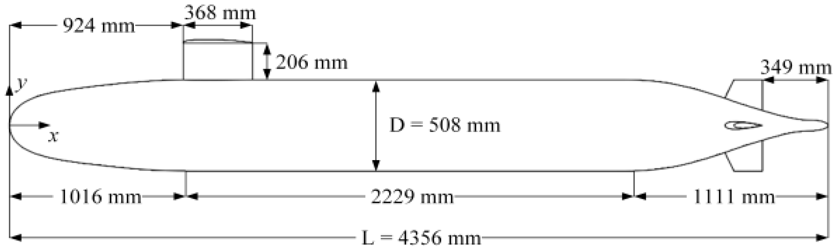
3.1. Model Geometry

In this paper, the 1:24 scaling SUBOFF model was used. The geometric model was based on the SUBOFF geometric model published by the David Taylor Research Center [21]. The total length of the model was 4356 mm, the head was 1016 mm, the middle part was 2229 mm, and the tail was 1111 mm. The leading edge of the sail was located at 924 mm of the submarine, the length was 368 mm, and the height was 206 mm. The trailing edge of the stern appendage was 349 mm away from the tail end of the submarine, which was arranged in a cross shape. The SUBOFF model is shown in Figure 1.

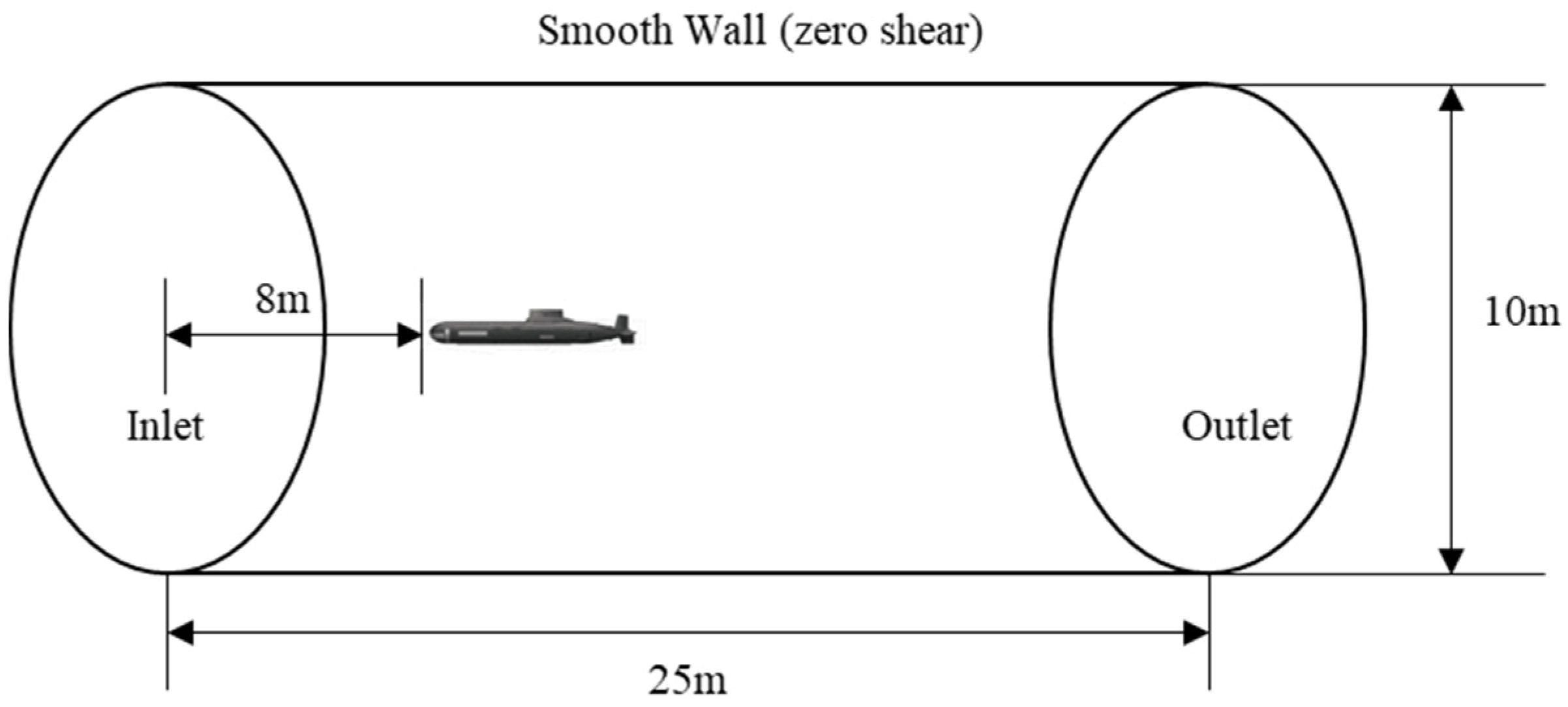
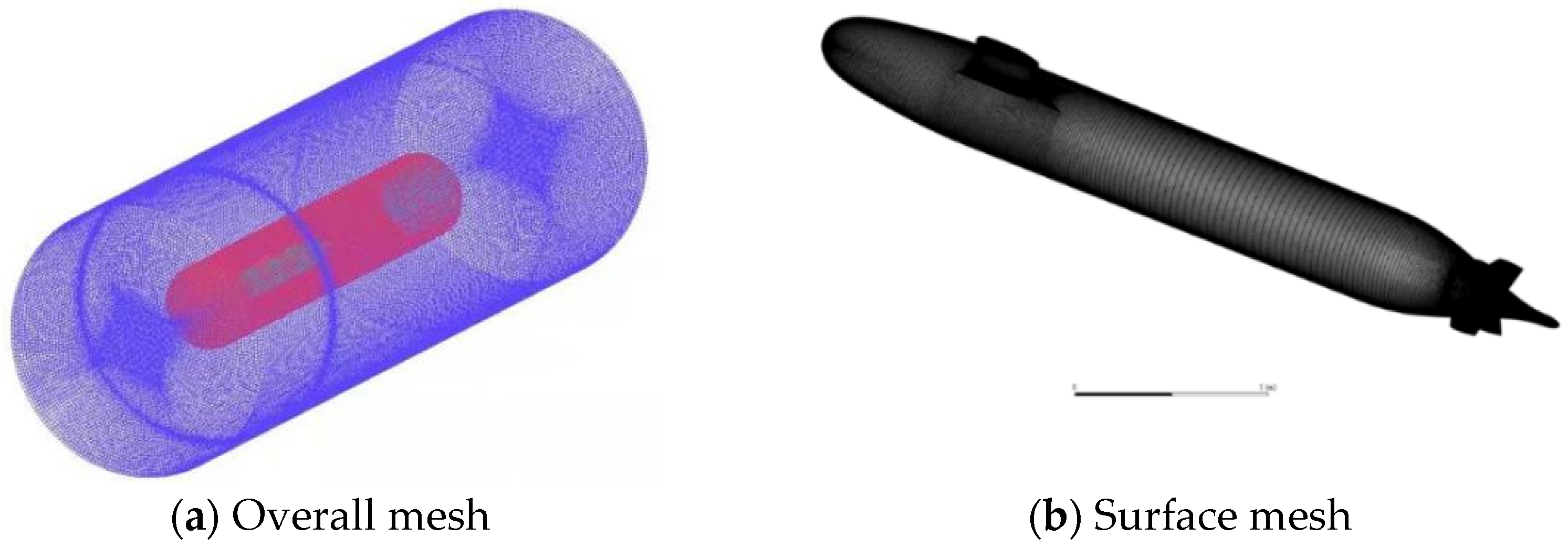
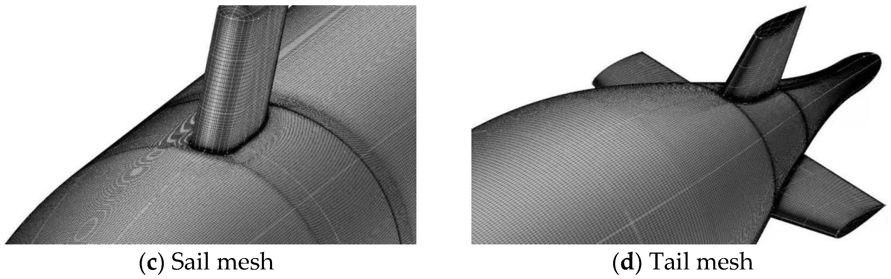
3.2. Mesh and Numerical Setup

The entire computational domain was divided into two subdomains: the inner domain and outer domain. The outer domain is shown in Figure 2. The submarine worked in a cylinder tunnel with a length of 25 m, and a radius of 10 m. The blockage ratio of the water domain was 0.0025, which was small enough that the blockage effect of the SUBOFF model could be ignored. The inlet was located 8 m upstream of the submarine. For the outlet boundary, it was defined as the pressure outlet boundary. Smooth wall conditions (zero shear) were defined as the side of the cylinder boundary, and the SUBOFF surface was considered to be the no-slip wall.

In order to obtain better turbulent structural characteristics of the submarines, mesh densification was carried out on the sail, the tail rudder, and the tail area. Meanwhile, considering the calculation power, the entire computing domain was divided into two parts: the inner domain and the outer domain. By refining the mesh, the outer domain can appropriately reduce the number of elements, so that the mesh can be effectively concentrated around the submarine. The submarine mesh is shown in Figure 3. In the numerical simulation of the submarine, high-quality results can be obtained only when all boundary layer solutions are sufficient. In this paper, the y+ was set to 1, the width of the first cell to the wall y was set to $1\times {10}^{-5}$ m, and it increased exponentially according to 1.1.

3.3. Verification of Mesh

The mesh density and quality have an important influence on the calculation results, and CFD uncertainty analysis was carried out with the numerical results of the submarine drag. Three groups of meshes were generated for verification, having approximately 23 million (coarse mesh), 44.3 million (medium mesh), and 82 million (fine mesh) cells. The verification simulations are presented at an operating velocity of 5.98 kn.

Table 1. The calculation results of the total drag coefficient.

Mesh Groups	ID	Number (M)	Drag Force (N)
Coarse	1	23	97.3
Medium	2	44.3	99.6
Fine	3	82	100.7

lists the number of meshes with different scales and resolutions.

Next, two steps were performed to complete the mesh-independent verification.

Step 1: Calculate the convergence ration R_k according to the following formula:

$$R_k={\epsilon }_{k32}/{\epsilon }_{k21}$$

(7)

$${\epsilon }_{k32}=S_{k3}-S_{k2}$$

(8)

$${\epsilon }_{k21}=S_{k2}-S_{k1}$$

(9)

where ${\epsilon }_{k21}$ is defined as the changes between ID1 and ID2, in the same way as ${\epsilon }_{k32}$.

The R_k = 0.4783. Because 0 < R_k < 1, the three different meshes presented monotone convergence, and the convergence was satisfied.

Step 2: Calculate the order of accuracy and one-term estimates:

$$p_{k1}=\frac{\ln \left({\epsilon }_{k32}/{\epsilon }_{k21}\right)}{\ln \left(r_k\right)}$$

(10)

$${\delta }_{R{E}_{k1}}^{*}=\frac{{\epsilon }_{k21}}{r_k^{p_{k1}}-1}$$

(11)

The correction factor C_k is

$$C_{k1}=\frac{r_k^{p_{k1}}-1}{r_k^{p_{kest}}-1}$$

(12)

Because C_k = 1.8572 >1, according to the ITTC (2017) recommendation, when the C_k >1, the mesh uncertainty U_k is

$$U_k=\left|C_{k1}{\delta }_{R{E}_{k1}}^{\ast }\right|+\left|\left(1-C_{Tk1}\right){\delta }_{R{E}_{k1}}^{\ast }\right|$$

(13)

The comparison error e_k is

$$E_k=D-S$$

(14)

The validation uncertainly U_v is

$$U_v=\sqrt{U_{SN}^2+U_D^2}$$

(15)

After calculation, E_k = 1.60, U_v = 3.42. For validation of the uncorrected simulation, |E_k| < U_v, so that the validation of U_v was achieved. Therefore, the medium met the requirement of mesh independence. Meanwhile, the result of the medium was 99.6 N, the experimental [22] result was 102.3 N, and the error was 2.64%, which met the requirements. Therefore, the mesh with 44.3 million was chosen for further simulation.

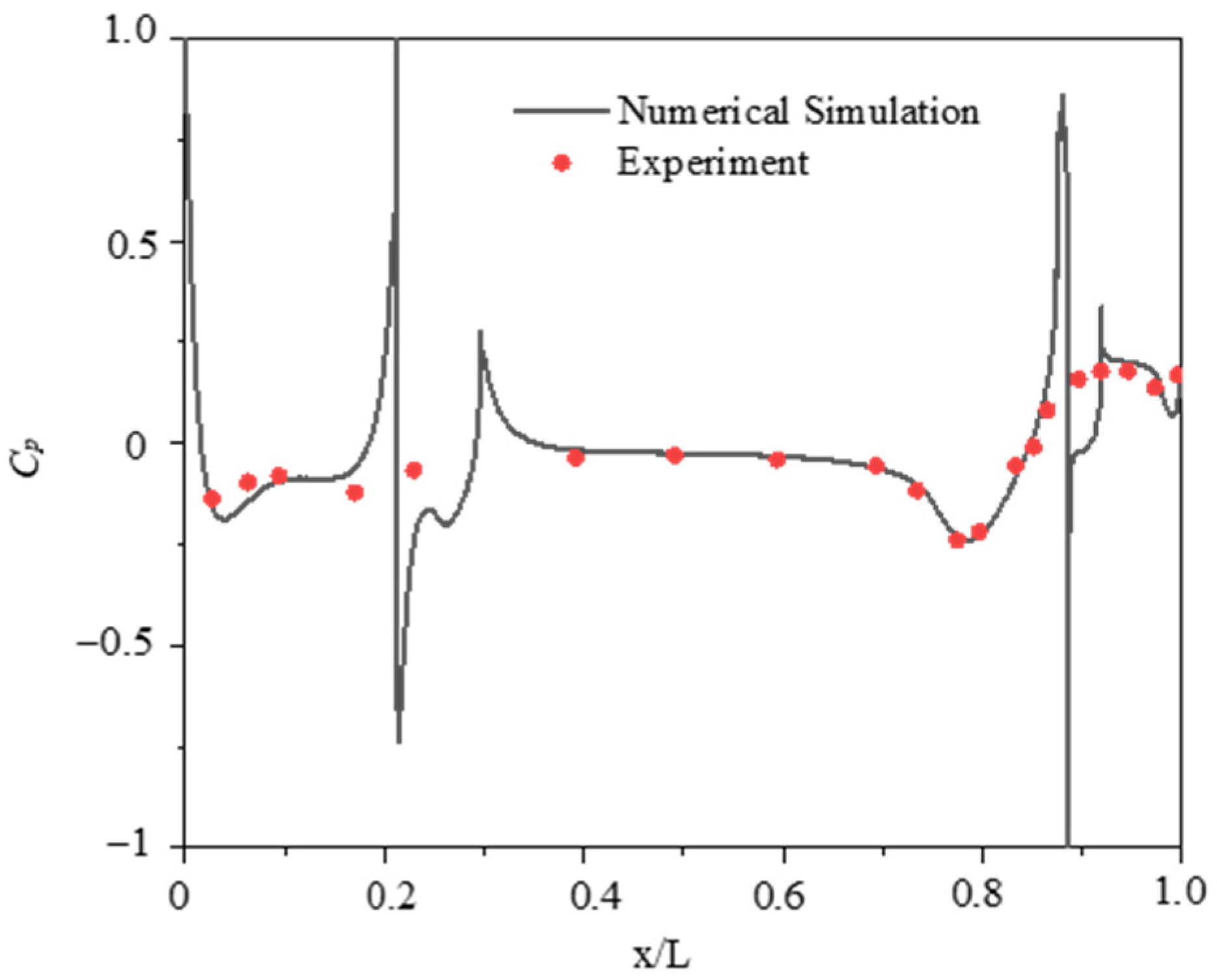
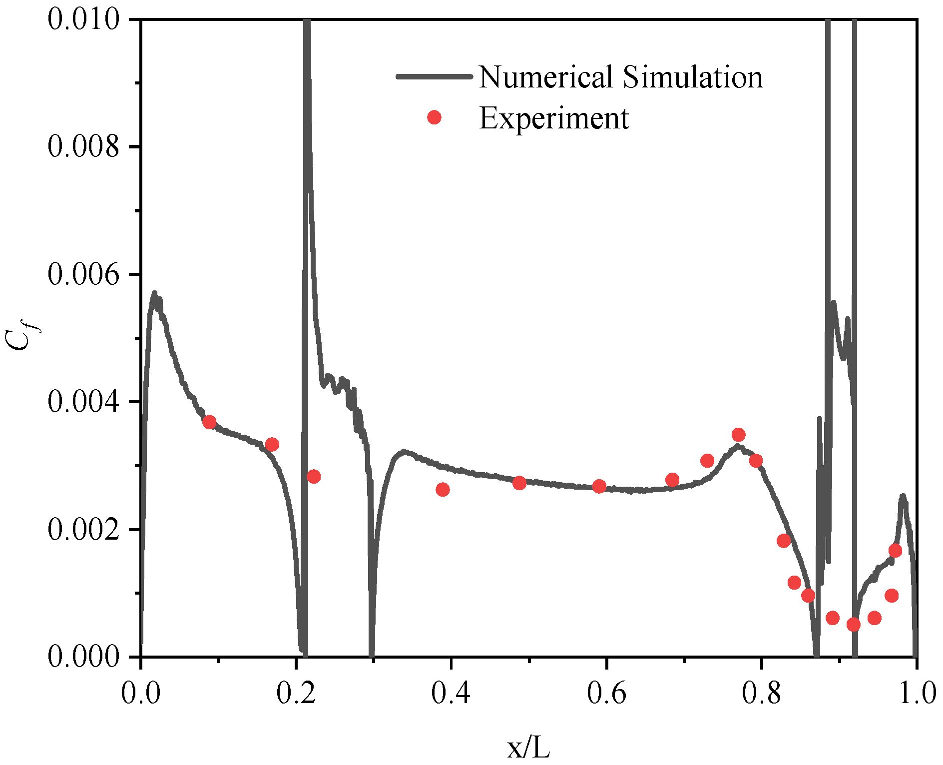
3.4. Verification of Numerical Method

In order to verify the validity of the numerical calculation method adopted in this paper, the numerical simulation under the working condition of 5.93 kn was carried out, and the results were compared with the experimental results [23], which were used to verify the pressure coefficient C_p and the surface friction coefficient C_f along the upper meridian line of the submarine longitudinal section obtained by numerical simulation. The formulas of C_p and C_f are shown as follows:

$$C_p=\frac{p-p_{ref}}{0.5{\rho }_{ref}{\nu }_{ref}^2}$$

(16)

$$C_f=\frac{{\tau }_w}{0.5{\rho }_{ref}{\nu }_{ref}^2}$$

(17)

where p is the static pressure; ${\tau }_{\omega }$ is the wall shear stress; $p_{ref}$ is the reference pressure; ${\rho }_{ref}$ is the reference density; and $v_{ref}$ is the reference velocity, in this paper, $v_{ref}$ refers to the flow velocity.

It can be seen from Figure 4 and Figure 5 that C_p and C_f are in good agreement with the experimental value. The pressure coefficient C_p values of the bow, the sail, and the tail of the SUBOFF were larger, while the C_p values of other parts of the submarine were smaller, which is consistent with the actual flow field. It was noted that the lift force was the integral of the pressure on the surface of the submarine, so it can be represented with the integral of the pressure coefficient. The experimental [23] value was −0.03615 and the calculated value was −0.03721. The error was 2.93%, which met the requirement of less than 5%.

Through the comparison, it could be found that the numerical calculation in this paper was in good agreement with the experimental results, which verifies the accuracy and feasibility of the numerical method used in this paper.

4. Results and Discussion

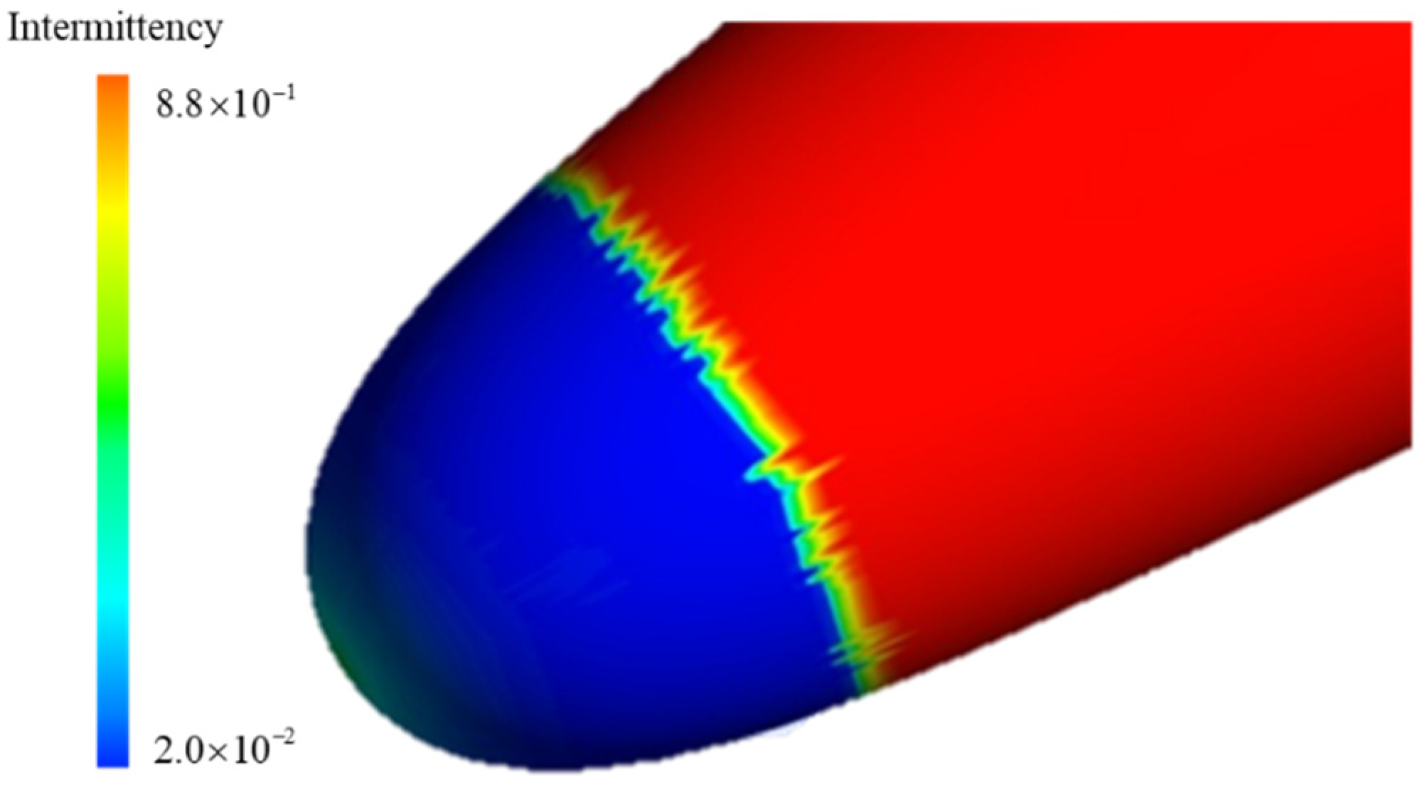
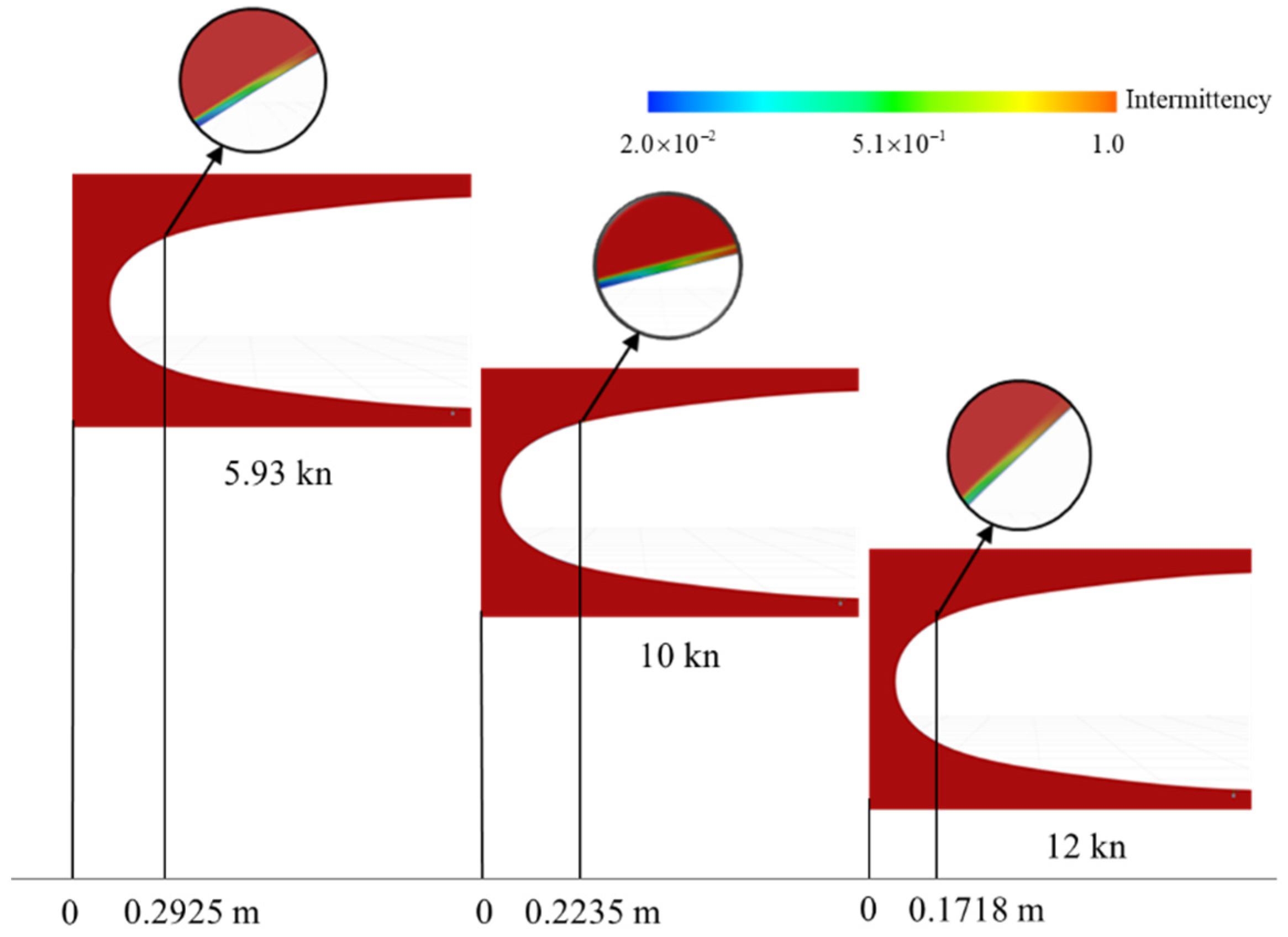
4.1. Overview of the Fluid and the Boundary Layer Transition

In this section, the characteristics of the overall and bow flow field of the submarine under three velocities (5.93 kn, 10 kn, 12 kn) were studied. Figure 6 shows the simulation results of the three pressures. It can be seen that the pressure distribution on the surface of the submarine was similar under three velocities. The places where the pressure changed strongly were the bow, the front of the sail, and the front of the tail, which is consistent with the actual flow field. According to Bernoulli’s principle, the impact of the fluid on the wall caused the velocity to decrease and the pressure to increase.

The surface distribution of the velocity gradient tensor under three velocities was the second invariant, as seen in Figure 7, where V_A denotes the inflow velocity. The vortex structure around the submarine was clearly visible, which could well capture the horseshoe vortex and top vortex pair at the bottom of the sail and the bottom of the rudder.

Table 2. The drag and structural parameters of the horseshoe vortex at three velocities.

Velocity (kn)	ReL	Fx (N)	Cd	A (m2)	Γ (m2/s2)
5.93	1.322 × 107	99.6	0.106	8.195 × 10−5	5.397 × 10−4
10	2.230 × 107	262.2	0.098	7.902 × 10−5	1.482 × 10−3
12	2.676 × 107	370.7	0.096	7.528 × 10−5	1.815 × 10−3

compares the total drag, the drag coefficient, and main parameters of the horseshoe vortex in the sail of the submarine under three velocities, where Re_L is the Reynolds number with the length as the characteristic length; F_x is the drag; C_d is the drag coefficient; A and Γ are the size of the vortex and the flux of the circulation as the flow direction vorticity, respectively. Γ is expressed as

$$\mathrm{\Gamma }={\displaystyle \underset{A}{\iint }{w}_x}dA$$

(18)

where ${\omega }_x$ is the vorticity component along the x-axis perpendicular to the measurement plane.

It can be seen from Table 2 that as the velocity increased, the drag on the submarine increased, the drag coefficient decreased slightly, and the structure of the horseshoe vortex in front of the sail became smaller, but the strength of the vortex increased.

Extracting the pressure coefficient distribution on the ridge of the longitudinal profile in the submarine, we compared the pressure coefficient of 5.93 kn with [23], which was closer to the literature results. Here, it can be seen that for the SUBOFF standard model, the velocity had essentially no effect on the distribution of the pressure coefficients (Figure 8), and the pressure coefficients for all three velocities reached their lowest values at x/L = 0.025.

Table 3. The parameters of the transition point at different velocities.

Velocity (kn)	S (m)	Res
5.93	0.2925	8.880 × 105
10	0.2235	1.144 × 106
12	0.1718	1.056 × 106

shows the specific location of the turning point calculated by the intermittent factor under the three cases. S is the arc length to the transition point at the bow, and Re_s is the Reynolds number with S as the characteristic length. As can be seen from the table, with the increase in the velocity, the position that reached the critical Reynolds number moved forward, so the turning point position moved forward gradually. The intermittency phenomenon occurred as the boundary layer developed along the flow direction from laminar to fully developed turbulence, that is, during the transition between laminar and turbulent periods. The intermittency factor is typically used to describe the intermittent phenomena. Intermittent phenomena can also occur in the normal upward direction such as in the areas where turbulent patches arise, where the turbulence is fully developed inside the patches, and the laminar is outside the patches. The intermittency factor $\gamma$ is the time average of the intermittency function I(x,y,z,t), which has a value of 0 in laminar flow and 1 in turbulent flow. The relationship between the two is expressed as

$$\gamma =\frac{1}{T}{\displaystyle \underset{0}{\overset{T}{\int }}I\left(x,y,z,t\right)}\mathrm{dt}=\gamma \left(x,y,z,t\right)$$

(19)

Figure 9 depicts the distribution of the bow’s intermittent factor, and the position of the transition point of the 1:24 scaling model of SUBOFF at 5.93 kn could be obtained. The arc length of the surface through which the fluid flowed was 0.2925 m at x = 0.20 m. Taking the arc length as the characteristic length, the critical Reynolds number Re_s = 8.880 × 10⁵ was obtained. The distribution of the intermittency factor allowed us to observe the location where the transient occurred, where the higher the velocity, the more forward the transition location, and Figure 10 shows the distribution of the intermittency factor at different velocities.

Figure 11 shows the time-averaged velocity profiles at the positions of x = 0.03 m, 0.087 m, 0.2 m, and 0.5 m, respectively. Based on the previously obtained positions of the transition points, when x < 0.0976 m, the boundary layers of the three cases were in laminar flow and the velocity distribution curves had inflection points, as shown in Figure 11a,b. When x = 0.2 m (Figure 11c), the case of 5.93 kn was still laminar, while the 10 kn and 12 kn were already after the turning point, and the distribution of the 10 kn and 12 kn velocities along the normal direction at this time also showed the typical turbulent boundary layer velocity profile characteristics. When x = 0.5 m (Figure 11d), the boundary layer of all three cases developed into a turbulent state, and the boundary layer was no longer a single laminar structure, but an inner and outer layer, and the velocity distribution profiles of the linear bottom layer, transition layer, logarithmic layer, and outer layer were characterized. This significant change in the velocity pattern is that the velocity profile with flow direction is an important sign of the boundary layer transition phenomenon.

Figure 11d shows the distribution of the turbulent boundary layer velocity along the normal direction at x = 0.5 m, where the velocity stratification structure of the inner layer was consistent with the wall rate of the turbulent boundary layer at the linear bottom layer ($0\le y^{+}\le (5~8)$), with

$$u^{+}=y^{+}$$

(20)

In the logarithmic layer ($(30~50)\nu /{\mu }_{\tau }\le y\le 0.2\delta$), the velocity distribution satisfies the logarithmic law of the form:

$$u^{+}=\frac{1}{\kappa }\ln y^{+}+C$$

(21)

Since there is still no consensus on the choice of coefficients, the calculated results of the three cases were fitted here, and 1/κ and C are shown in

Table 4. The fitting results of 1/κ and C.

Velocity (kn)	1/κ	C
5.93	3.1379	1.9797
10	3.1086	1.5708
12	3.1146	1.5411

. Combined with Figure 11d, it is clear that at the same flow position, in the inner layer with y < 0.2δ, the profiles of the boundary layer with various mainstream velocities were very similar and did not change significantly with the change in velocity. While in the outer layer with y > 0.2δ, the data points for different mainstream velocities fell on different profiles, and the appearance of this dispersion implies a change in the turbulence characteristics.

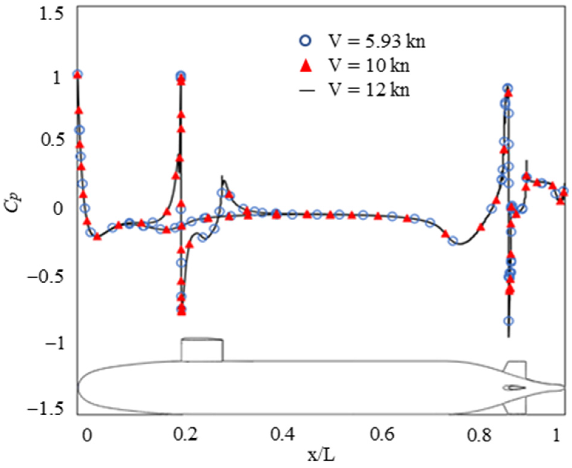
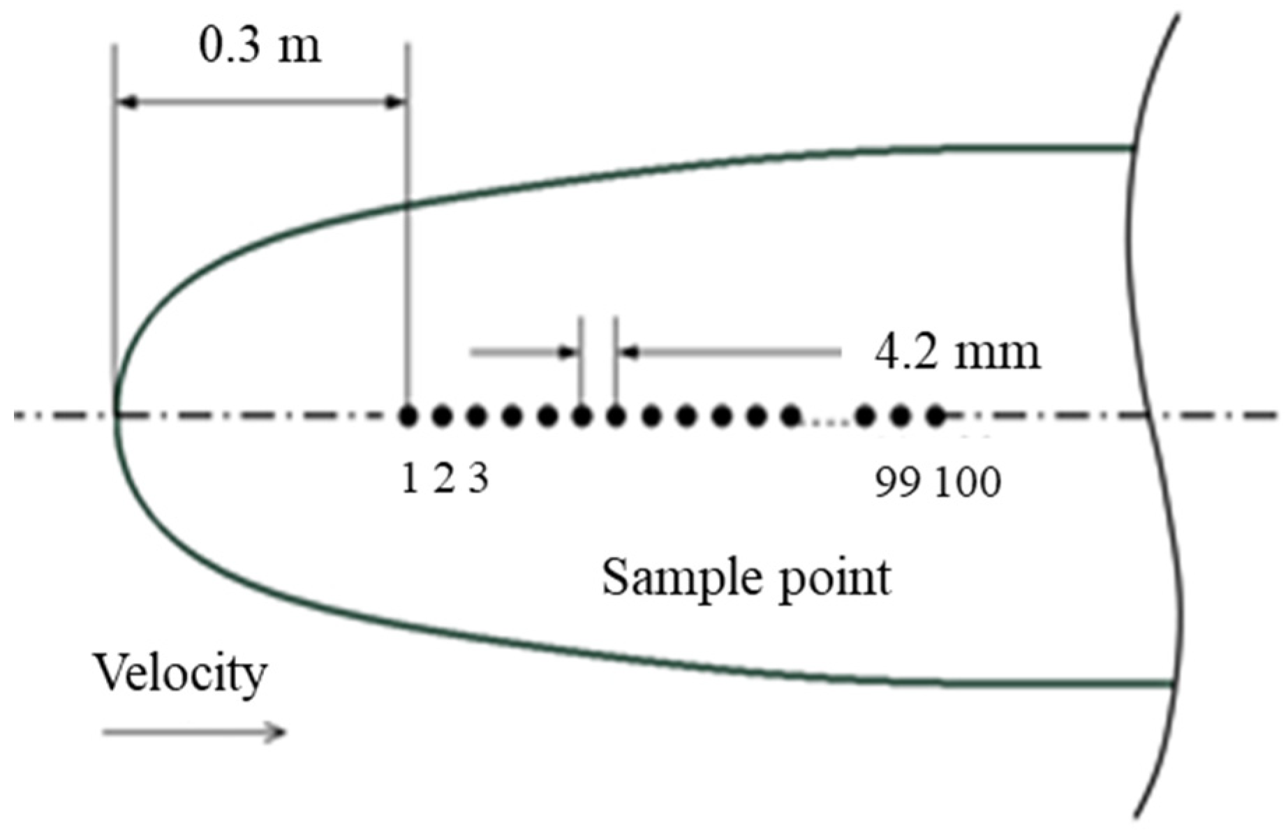
4.2. Axial Pressure Distribution

As shown in Figure 12, thirty sample points were arranged along the mid-longitudinal profile ridge on the surface of the bow. Figure 13 shows the curves of the pressure fluctuation at several of the selected sample points with time. Due to the small velocity, the pressure fluctuation at different flow locations was not visually distinguishable in the time domain, so Cp′ is needed to be used to measure the magnitude of the pressure fluctuation, which represents the strength of the pressure fluctuation, and is expressed as

$$C{p}^{\prime }=\frac{p_{rms}^{\prime }}{Q_v}\times 100\%$$

(22)

where $p_{rms}^{\prime }$ is the root mean square value of pressure fluctuation; $Q_v$ is the pressure of the fluid velocity.

The pressure fluctuation data at the bow were extracted for the three cases, and the variation curves of the pulsation pressure with times at several sample points at 12 kn are shown in Figure 13. At a higher velocity of 12 kn, it can be observed from the time domain that the amplitude of pulsation pressure was very small in the laminar region, there was a sudden increase in the transient region (Re_s = 1.011 × 10⁶), and then there was a certain decrease in the turbulent region, but it was still higher than the laminar.

Figure 14 gives the strength of the pressure fluctuation at different velocities for the first 20 sample points along the axial direction at three velocities. This is in agreement with the time-domain characteristics where the pressure fluctuation is small in the laminar region and has a clear peak at the transient region, after which it decays rapidly and develops to the turbulent phase, where the pressure fluctuation magnitude is maintained at a lower level, but is somewhat larger than in the laminar. This feature of the boundary layer pressure fluctuation is also one of the most effective methods to detect boundary layer transitions. For example, Hu et al. [24] used the pulsation pressure test technique to detect the boundary layer transitions in a 10° cone in a wind tunnel and obtained the evolution of the pulsation pressure coefficient along the bus.

Comparing the pressure fluctuation evolution law for three velocities, the transition point at the bow moved forward with increasing velocity and the pressure fluctuation coefficient declined, while the strength of the pressure fluctuation in the transient region increased, and the magnitude of the increase grew larger. In conclusion, the pressure fluctuation strength in the transient area may be separated from the laminar and turbulent flow more clearly when the velocity is higher.

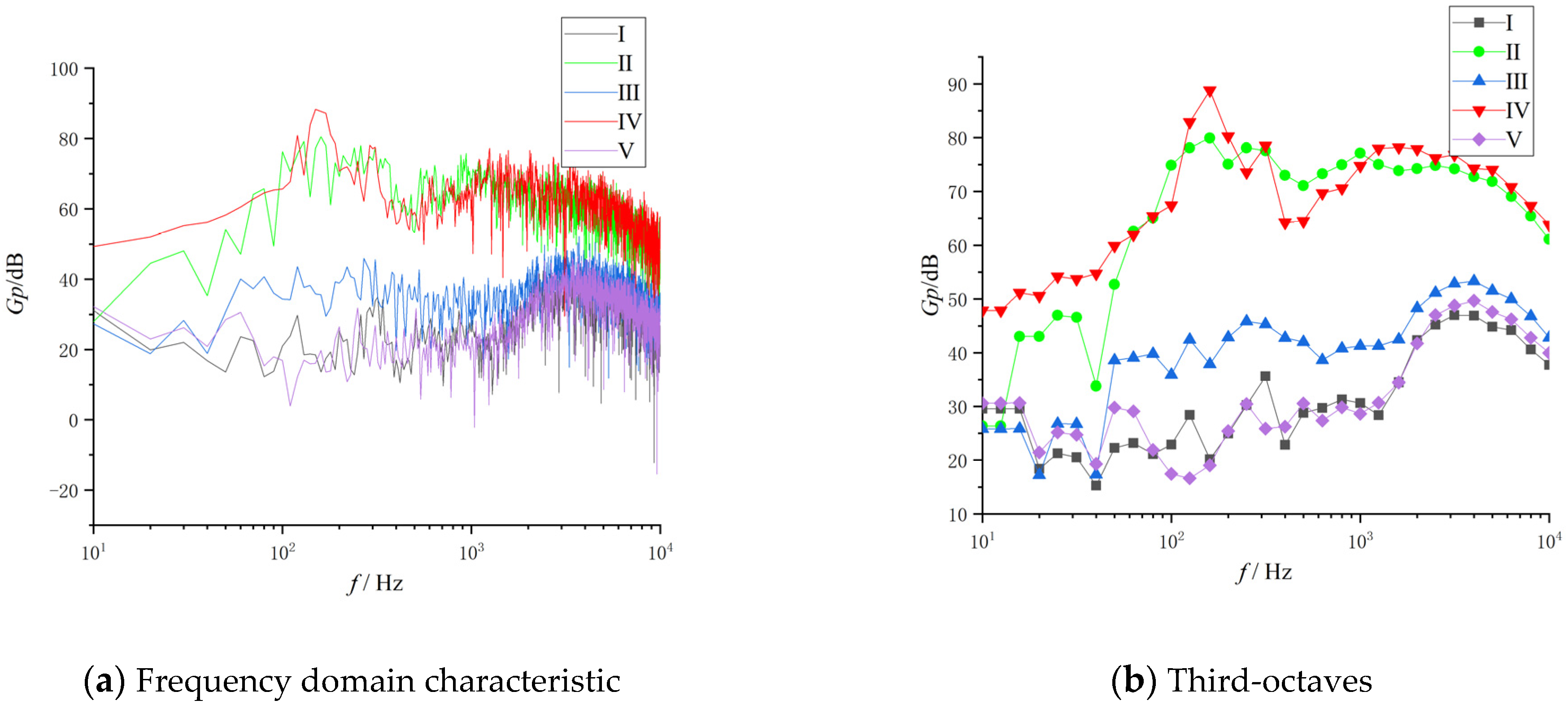
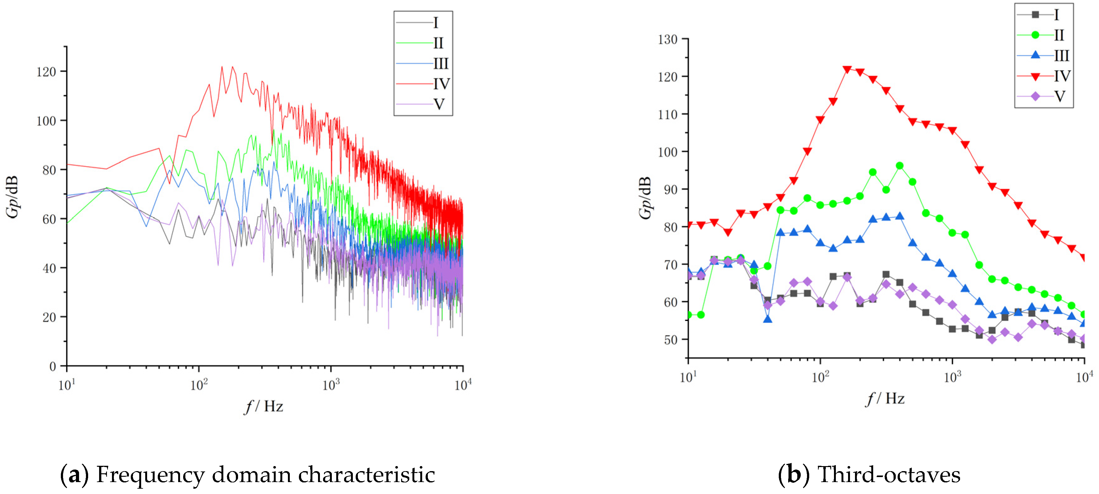
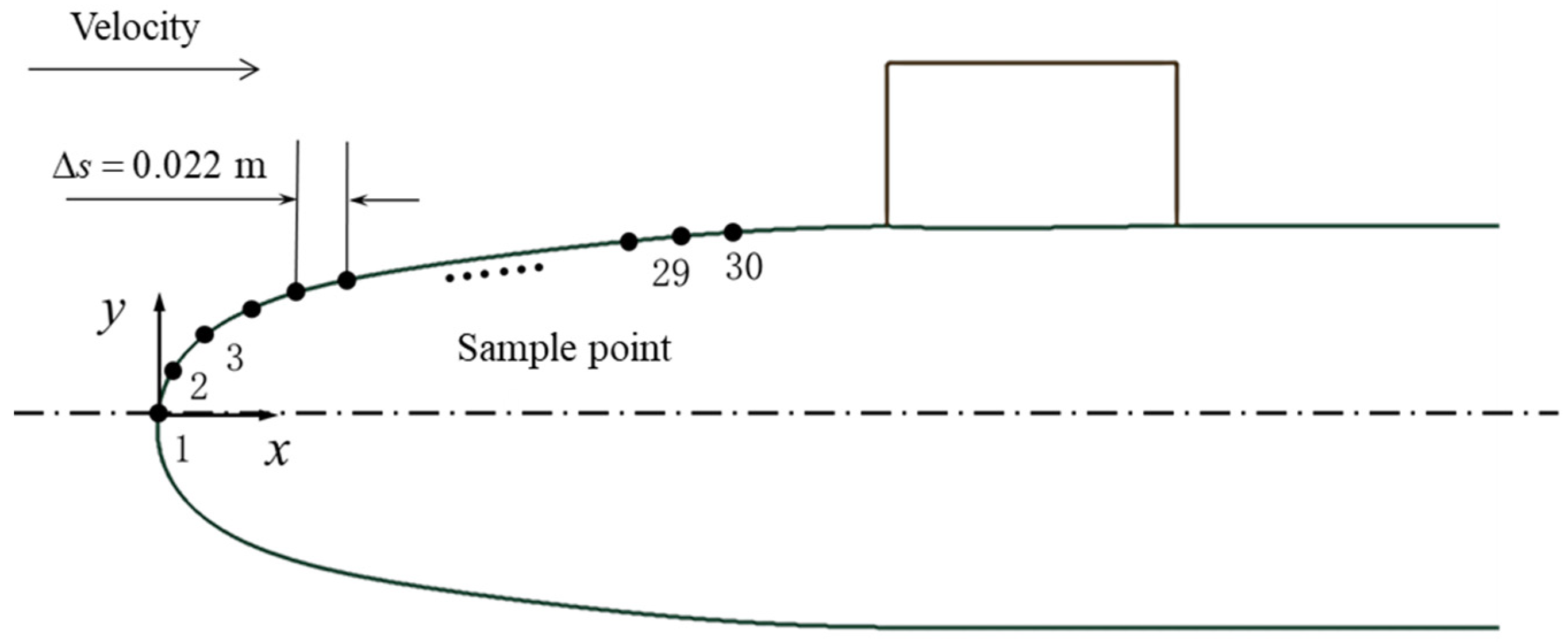
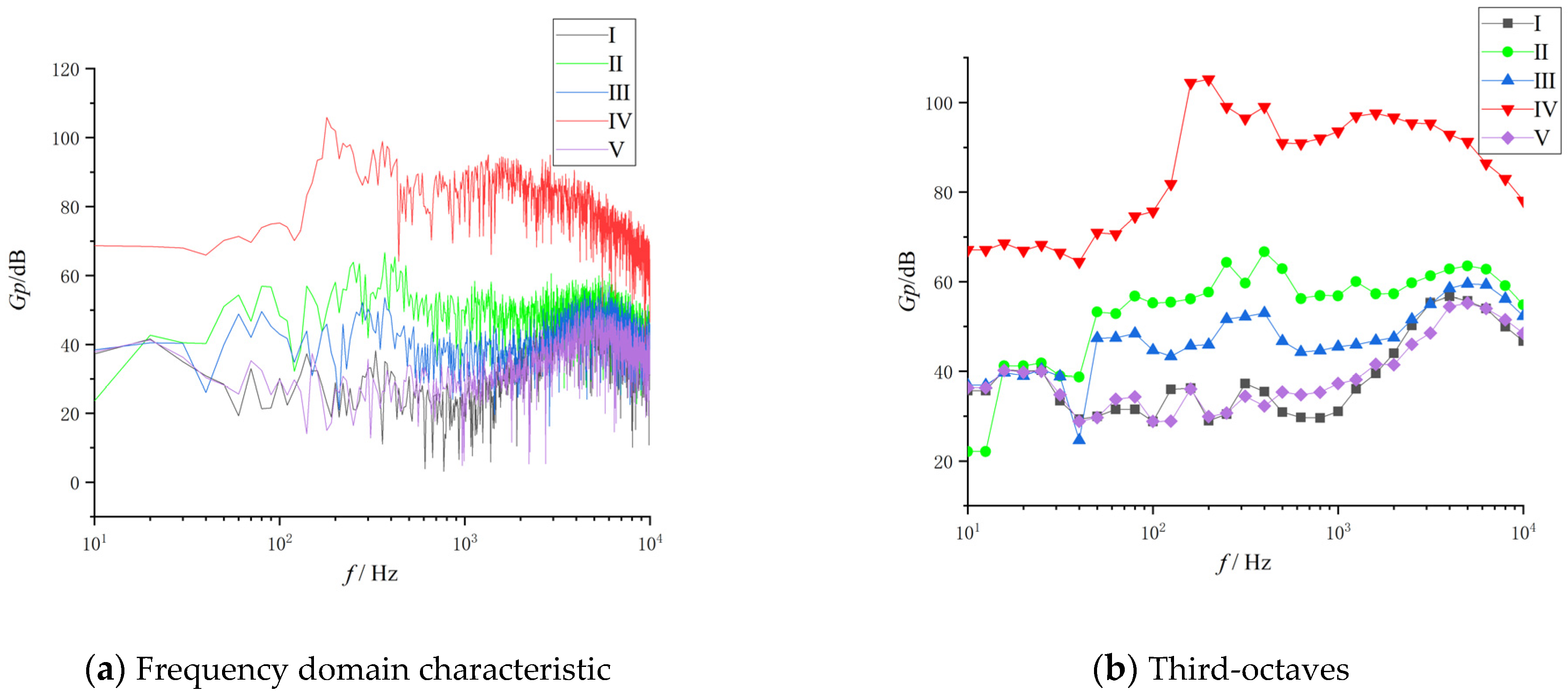
4.3. Self-Power Spectral of Wall Pressure Fluctuation

The self-power spectral of the pressure fluctuation at the sample point at different velocities is given in Figure 15, Figure 16 and Figure 17. According to Parseval’s theorem, the total energy of the signal in the time domain was equal to the total energy of the signal in the frequency domain. From the random signal through Fourier transform, and then through the following calculation, we could find its self-power spectrum. In this paper, the frequency characteristics of the pressure fluctuation are represented by the power spectrum G_p and is defined as

$$G_p=10\lg \frac{G\left(f\right)}{p_{ref}^2}$$

(23)

where p_ref is baseline sound pressure; p_ref = 1 $\mu$ pa; G(f) is the pressure fluctuation power spectral density function calculated with fast Fourier transform.

In the low- and medium-frequency range, each velocity case followed the same pattern of the highest spectral level occurring in the transient region, the lower spectral level in the region toward turbulence, and the lowest spectral level in the laminar region. In the frequency range around 100 Hz, a peak gradually appeared during the development from the laminar to the transient, which was associated with the T–S wave generated in the sensible phase and growth in the linear phase. The frequency and spectral level of this peak at each velocity transient point are given in

Table 5. The parameters of the T–S wave at different velocities.

	5.93 kn	10 kn	12 kn
fTS (Hz)	93.33	133.33	166.67
Spectrum level (dB)	135.70	141.84	149.92

. It is clear that as the velocity rises, the T–S wave frequency and spectral level increased.

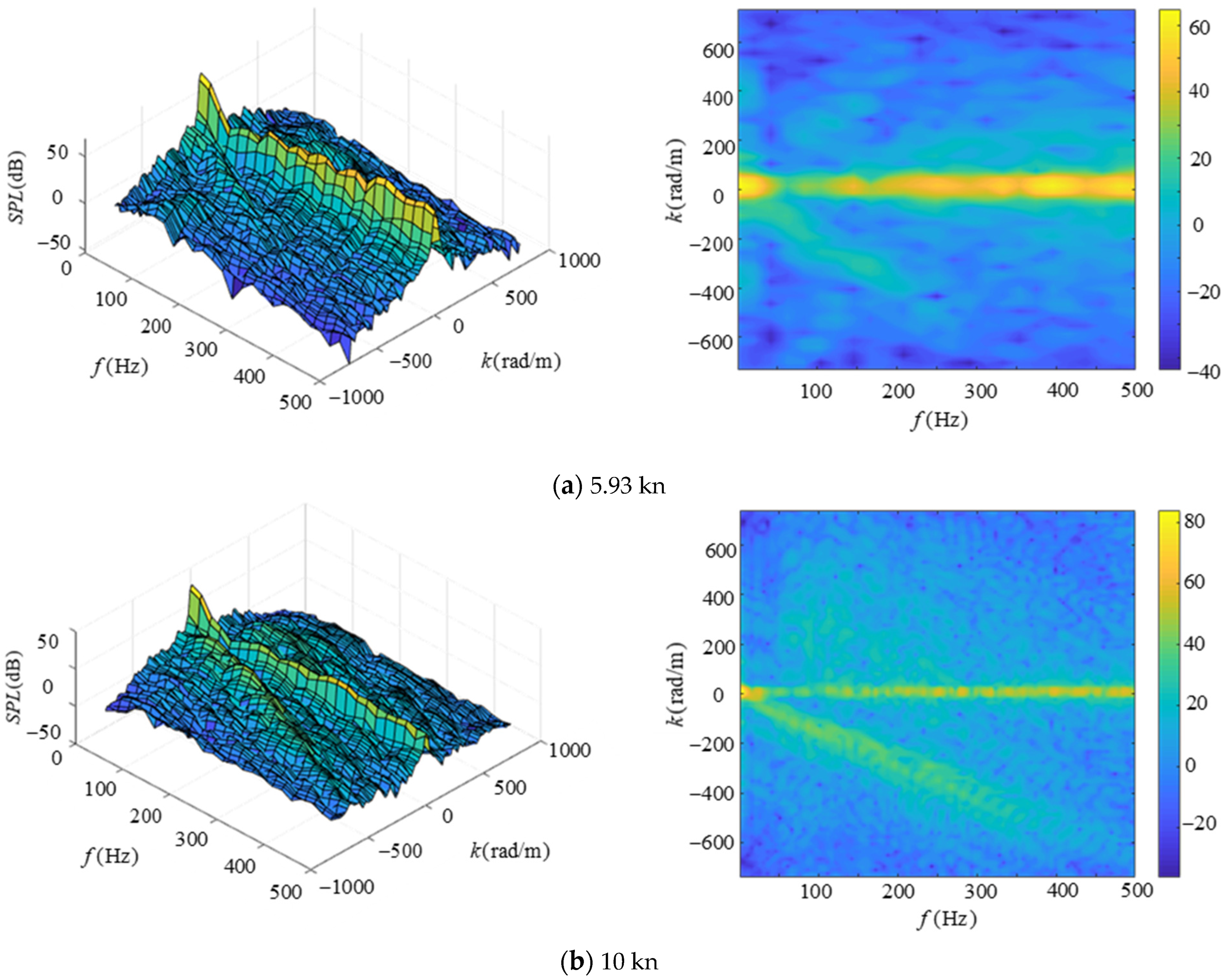
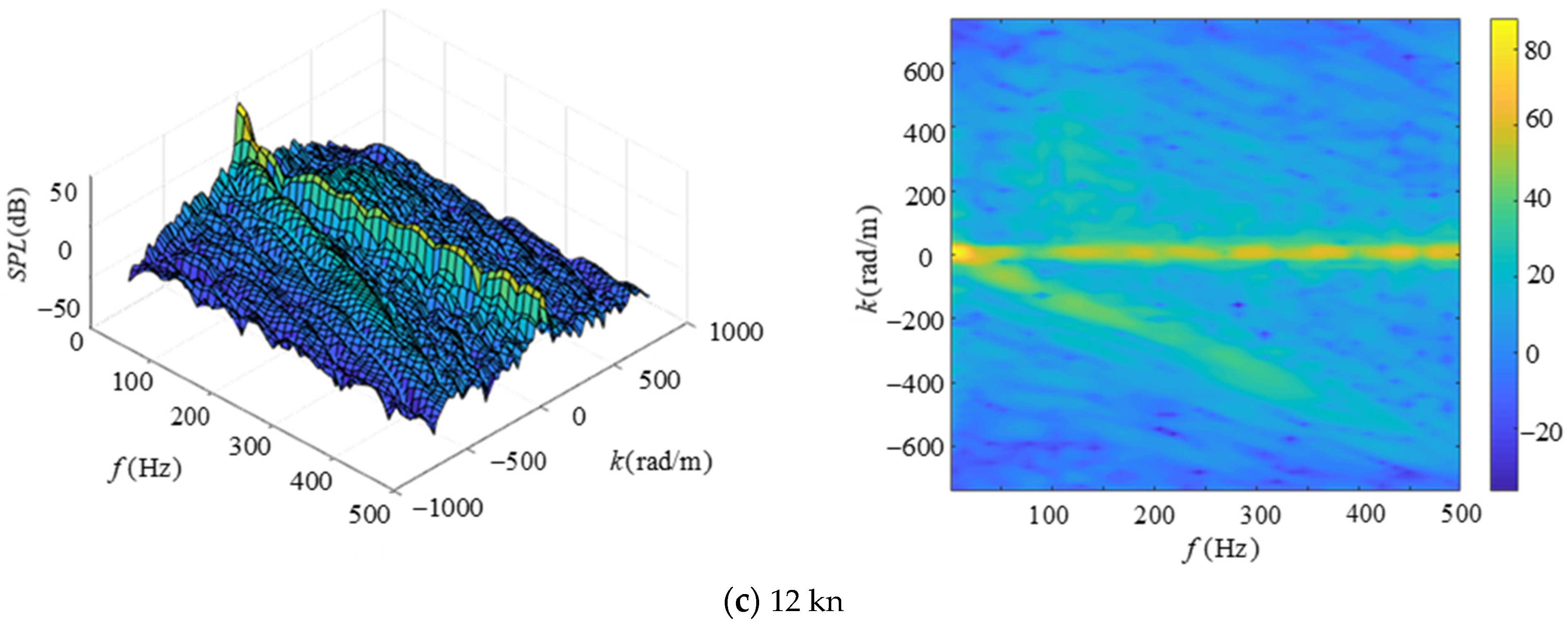
4.4. Wave-Number Frequency Spectrum of Wall Pressure Fluctuation

The pressure fluctuation was subjected to a two-dimensional Fourier transform from time–space to the wave-number frequency domain in order to examine the movements of the bow turbulent boundary layer vortices and the distribution of energy. With a sampling time step of 0.001 s, only the low-frequency portion of the spectrum, which corresponds to the large-scale eddies, was studied in this paper.

Fourier transform of the correlation function of the turbulent pressure fluctuation time-space signal was used to define the wave-number frequency spectrum. The equation is as follows:

$$\mathrm{\Phi }\left(\overrightarrow{k},w\right)={\displaystyle {\int }_{-\infty }^{+\infty }R\left(\overrightarrow{\xi },\tau \right)}{e}^{-i\left(\overrightarrow{k},\overrightarrow{\xi }+\omega \tau \right)}d\overrightarrow{\xi }d\tau$$

(24)

By applying a fast Fourier variation to the discrete spatial and temporal signals of turbulent pressure fluctuation and methodically averaging the square of its amplitude, it is typically possible to derive the wave-number frequency spectrum in practice. The formula is:

$${\mathrm{\Phi }}_m\left(k,w\right)=\frac{\langle {\left|{\displaystyle \sum _{n=1}^N{\displaystyle \sum _{m=1}^{M}W\left(x_m,t_n\right)p_m\left(x_m,t_n\right)e^{-i\left(k_x{x}_m+w{t}_n\right)}\Delta x\Delta t}}\right|}^2\rangle }{{\left(2\pi \right)}^{2}NM{C}_w}$$

(25)

where p_m is the pressure fluctuation from the mth sensor. N is the number of time nodes and M is the number of sensors. ∆x is sensor spacing and ∆t is the time step.

$$x_m=\left(m-1\right)\Delta x$$

(26)

$$t_n=\left(n-1\right)\Delta t$$

(27)

$$W\left(x_m,t_n\right)=W\left(x_m\right)W\left(t_n\right)$$

(28)

where $W\left(x_m\right)$ and $W\left(t_n\right)$ are window functions. The Hanning window was used in this paper.

$$C_w=\frac{{\displaystyle \sum _{n=1}^N{\displaystyle \sum _{m=1}^M{W}^2\left(x_m,t_n\right)}}}{NM}$$

(29)

In the wave-number domain, the range was −π⁄d to π⁄d with a resolution of 2π/Nd, where D is the distance between adjacent sampling points and N is the number of sampling points. With an interval of 4.2 mm between adjacent monitoring points, 100 points were placed along the ridge line of the mid-longitudinal profile in the fully developed turbulent area at the bow to increase the resolution of the wave-number domain. According to Figure 18, the first sample point was situated at x = 0.3 m.

Figure 19 shows the wave-frequency spectrum of the wall pressure fluctuation at three velocities. The acoustic component is what led to the highest value at k = 0. It is clear that the migratory ridge was readily visible. With an increase in frequency, the amplitude lowered, the wave number decreased to the peak value of the migration ridge, and the migration ridge widened. The highest portion of the wavenumber-frequency spectrum, or the distribution of energetic vorticity with the highest energy, had a frequency domain range that expanded with increasing velocity from the standpoint of energy distribution.

Table 6. The parameters of the wave-number frequency spectrum.

Item	5.93 kn	10 kn	12 kn
Spectral peak level (dB)	21.79	64.61	83.57
Frequency range (Hz)	(0,250)	(0,450)	(0,500)
Wavenumber range (rad/m)	(−529,0)	(−680,0)	(−695,0)
Migration rate (m/s)	2.17	3.62	4.49
Dimensionless migration rate	0.71	0.70	0.73

lists the computed results for the wave-number frequency spectrum parameters. The three velocities had peak spectral levels of 21.79 dB, 64.61 dB, and 83.57 dB, respectively. These values are consistent with the change in the self-power spectral level, which rises with increasing velocity. The migration velocity is one of the crucial physical quantities to examine the turbulent wall pressure, which reflects the motion velocity of the turbulent vortex cluster structure.

The calculated migration velocities for 5.93 kn, 10 kn, and 12 kn were 2.17 m/s, 3.62 m/s, and 4.49 m/s, respectively, while the corresponding dimensionless velocities were 0.71 m/s, 0.70 m/s, and 0.72 m/s, meaning that the migration velocities rose as the main flow velocities rose, while the corresponding dimensionless velocities hovered around 0.7.

5. Conclusions

For the SUBOFF standard model 5.93 kn, 10 kn, and 12 kn cases, calculations were carried out to determine the flow field structure and pressure fluctuation for various velocities. The following conclusions were drawn after data analysis.

(1)

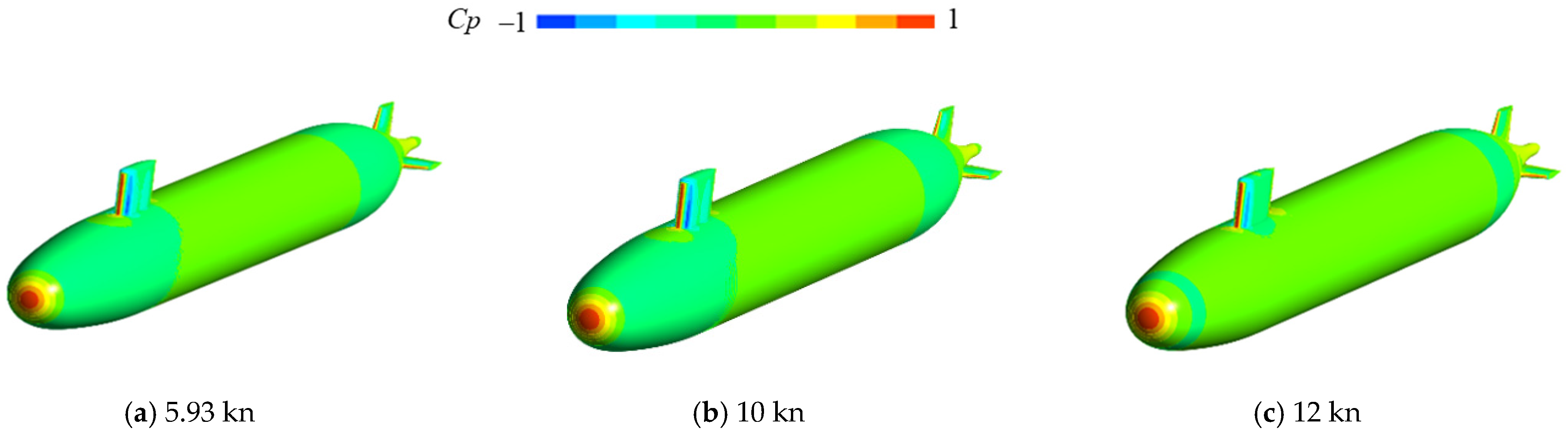
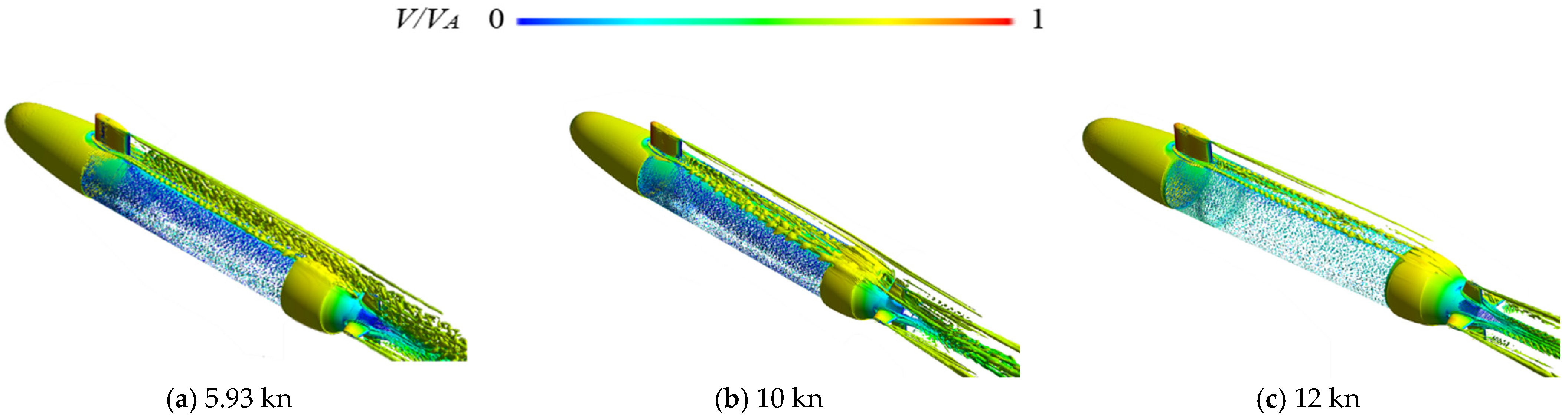
The distribution of pressure coefficients along the ridge of the mid-longitudinal profile and the distribution of pressure and velocity in the flow field of the submarine under various velocities essentially followed the same pattern. The influence of velocities on the flow field was more apparent in the numerical magnitude of pressure and velocity as well as the size and intensity of the vortex structure. With increasing velocity, the submarine experienced an increase in both the drag coefficient and the total drag force. However, the size of the horseshoe vortex at the sail deck’s bottom leading edge decreased as the velocity rose, and its intensity increased.

(2)

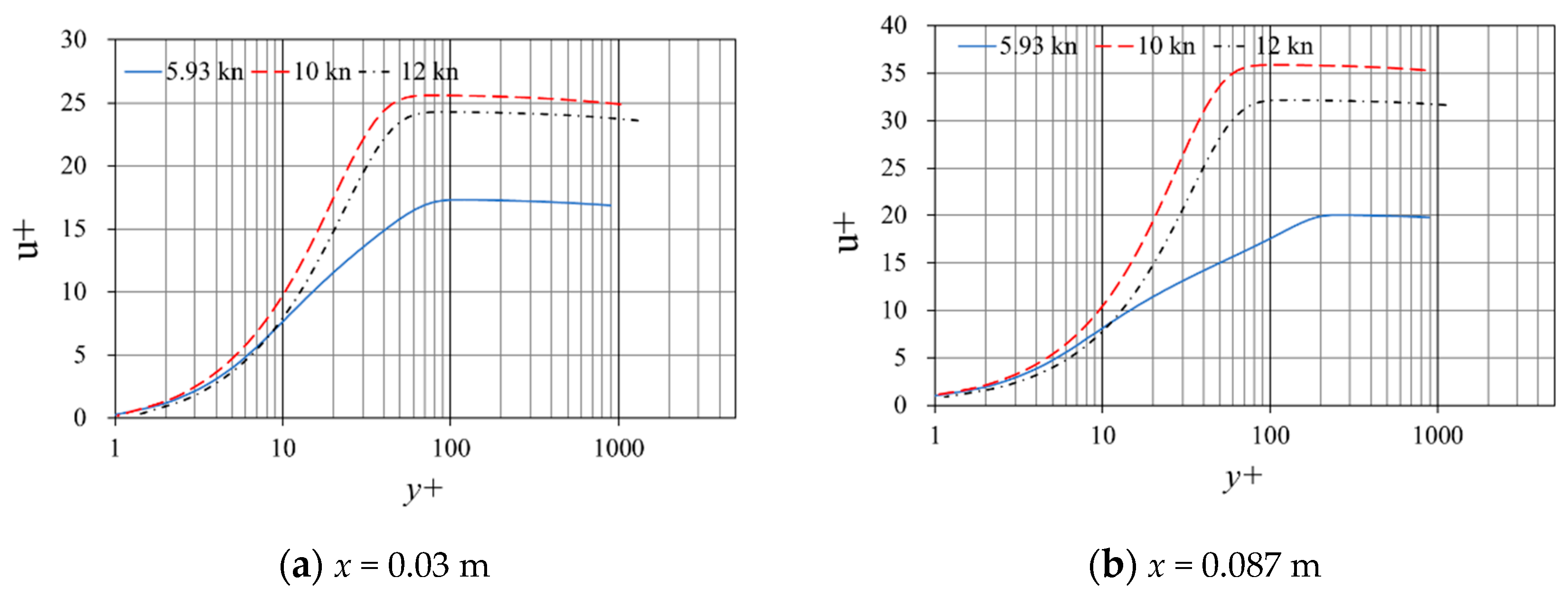
Using the horizontal distance to the stationary point of the bow as the characteristic length, the critical Reynolds number of the submarine’s bow was 6.339 × 10⁵. With the higher velocity, the crucial Reynolds number was positioned further ahead and the transient point was located farther forward.

(3)

When the transient occurred, the pressure fluctuation amplitude greatly increased and appeared to reach a high peak before swiftly decaying and dropping to a lower level in the turbulent region. The pressure fluctuation at the wall of the submarine’s bow was relatively modest in the laminar region. The peak obtained in the transient region rose under conditions of increasing velocity and advanced with it.

(4)

As the pulsation energy of each frequency component significantly increased at the transient compared to laminar flow, the magnitude of the pressure fluctuation was reflected in the self-power spectrum. During the development from laminar to the transient, a peak gradually appeared in the frequency range of about 100 Hz, which was associated with the T–S wave generated in the perceptive phase and growing in the linear phase. The T–S wave frequency rose with increasing velocity, and the spectral level followed suit.

(5)

In the fully developed turbulent region’s wave-number-frequency spectrum, a clear migration ridge with energy focused in the lower frequency range could be seen. The migration ridges increased in frequency, width, and amplitude as they migrated in the direction of lower wave numbers. The migration velocity was the vortex cluster’s average movement speed; the larger the velocity, the higher the migration velocity, which was maintained at 0.7.

References

1. Huang, T.; Liu, H. Measurement of flows over an axisymmetric body with various appendages in a wind tunnel: The DARPA SUBOFF experimental program. In Proceedings of the 19th Symposium on Naval Hydrodynamics, Seoul, Korea, 23–28 August 1992. [Google Scholar]
2. Saeed, A.; Ali, A.D.; Ali, S. Effects of bulbous bow on cross-flow vortex structures around a streamlined submersible body at intermediate pitch maneuver: A numerical investigation. J. Mar. Sci. Appl. 2016, 15, 8–15. [Google Scholar]
3. Manoha, E.; Troff, B.; Sagaut, P. Trailing-edge noise prediction using large-eddy simulation and acoustic analogy. AIAA J. 2000, 38, 575–583. [Google Scholar] [CrossRef]
4. Posa, A.; Balaras, E. A numerical investigation of the wake of an axisymmetric body with appendages. J. Fluid Mech. 2016, 792, 470–498. [Google Scholar] [CrossRef]
5. Broglia, R.; Posa, A.; Bettle, M. Analysis of vortices shed by a notional submarine model in steady drift and pitch advancement. Ocean Eng. 2020, 218, 108236. [Google Scholar] [CrossRef]
6. Ashok, A.; Buren, T.; Smits, A. The structure of the wake generated by a submarine model in yaw. Exp. Fluids 2015, 56, 123. [Google Scholar] [CrossRef]
7. Spalart, P. Detached Eddy Simulation. Annu. Rev. Fluid Mech. 2009, 41, 181–202. [Google Scholar] [CrossRef]
8. Alin, N.; Fureby, C. LES of the flow past simplified submarine hulls. In Proceedings of the 8th International Conference on Numerical Ship Hydrodynamics, Busan, Korea, 22–25 September 2003. [Google Scholar]
9. Alin, N.; Bensow, R.; Fureby, C. Current capabilities of DES and LES for submarines at straight course. J. Ship Res. 2010, 54, 184–196. [Google Scholar] [CrossRef]
10. Liu, Z.; Ying, X.; Tu, C. Numerical simulation and control of horseshoe vortex around an appendage–body junction. J. Fluids Struct. 2011, 27, 23–42. [Google Scholar]
11. Wang, X.; Huang, Q.; Pan, G. Numerical research on the influence of sail leading edge shapes on the hydrodynamic noise of a submarine. Appl. Ocean Res. 2021, 117, 102935. [Google Scholar] [CrossRef]
12. Magionesi, F.; Ciappi, E. Characterization of the response of a curved elastic shell to turbulent boundary layer. In Proceedings of the ASME 2010 3rd Joint US-European Fluids Engineering Summer Meeting and 8th International Conference on Nanochannels, Microchannels, and Minichannels, Montreal, QC, Canada, 1–5 August 2010. [Google Scholar]
13. Bhushan, S.; Alam, M.F.; Walters, D.K. Evaluation of hybrid RANS/LES models for prediction of flow around surface combatant and SUBOFF geometries. Comput. Fluids 2013, 88, 834–849. [Google Scholar] [CrossRef]
14. Magionesi, F.; Mascio, A.D. Investigation and modeling of the turbulent wall pressure fluctuation on the bulbous bow of a ship. J. Fluids Struct. 2016, 67, 219–240. [Google Scholar] [CrossRef]
15. Li, H.; Huang, Q.; Pan, G. An investigation on the flow and vortical structure of a pre-swirl stator pump-jet propulsor in drift. Ocean Eng. 2022, 250, 111061. [Google Scholar] [CrossRef]
16. Dietiker, J.F.; Hoffmann, K.A. Predicting wall pressure fluctuation over a backward-facing step using detached eddy simulation. J. Aircr. 2009, 46, 2115–2120. [Google Scholar] [CrossRef]
17. Meng, W.; Moin, P. Computation of trailing-edge flow and noise using large-eddy simulation. AIAA J. 2000, 38, 2201–2209. [Google Scholar]
18. Meng, W.; Moreau, S.; Iaccarinoand, G. LES prediction of wall-pressure fluctuations and noise of a low-speed airfoil. Int. J. Aeroacoustics 2009, 8, 177–198. [Google Scholar]
19. Menter, F. Stress-Blended Eddy Simulation (SBES)—A new paradigm in hybrid RANS-LES modeling. In Symposium on Hybrid RANS-LES Methods; Springer: Cham, Switzerland, 2016. [Google Scholar]
20. ANSYS. ANSYS 2020 R1 Fluent User Guide; ANSYS: Canonsburg, PA, USA, 2020. [Google Scholar]
21. Groves, N.C.; Huang, T.T.; Chang, M.S. Geometric Characteristics of DARPA (Defense Advanced Research Projects Agency) SUBOFF Models (DTRC Model Numbers 5470 and 5471); David Taylor Research Center Bethesda MD Ship Hydromechanics Dept.: Bethesda, MD, USA, 1989. [Google Scholar]
22. Liu, H.; Huang, T. Summary of DARPA SUBOFF Experiment Program Data; Naval Surface Warface Center, Cardrock Division (NSWCCD): Bethesda, MD, USA, 1999. [Google Scholar]
23. BULL, P. The validation of CFD predictions of nominal wake for the SUBOFF fully appended geometry. In Proceedings of the Twenty-First Symposium on Naval Hydrodynamics, Washington DC, USA, 24–28 June 1997. [Google Scholar]
24. Hu, C.; Huang, X. The location of boundary-layer transition detected by pressure fluctuation measurements. Exp. Meas. Fluid Mech. 2002, 2, 67–71. [Google Scholar]
Figure 1. The shape of the SUBOFF.
Jmse 10 01188 g001
Figure 2. Computational domain and boundary conditions.
Jmse 10 01188 g002
Figure 3. Mesh of SUBOFF.
Jmse 10 01188 g003aJmse 10 01188 g003b
Figure 4. Cp along the upper meridian line.
Jmse 10 01188 g004
Figure 5. Cf along the upper meridian line.
Jmse 10 01188 g005
Figure 6. The contours of pressure at three velocities.
Jmse 10 01188 g006
Figure 7. The instantaneous isosurface of the Q-criterion at three velocities.
Jmse 10 01188 g007
Figure 8. The distribution of the ridge pressure coefficients in the longitudinal profiles.
Jmse 10 01188 g008
Figure 9. The transition position at the velocity of 5.93 kn.
Jmse 10 01188 g009
Figure 10. The transition position at three velocities.
Jmse 10 01188 g010
Figure 11. The velocity distribution within the boundary layer at different normal positions of the bow.
Jmse 10 01188 g011aJmse 10 01188 g011b
Figure 12. The position of the axial sample points.
Jmse 10 01188 g012
Figure 13. The fluctuation of pressure over time at the velocity of 12 kn. (a) Res = 2.689 × 10⁵. (b) Res = 6.738 × 10⁵. (c) Res = 1.011 × 10⁶. (d) Res = 1.482 × 10⁶. (e) Res = 2.561 × 10⁶.
Jmse 10 01188 g013
Figure 14. At three velocities.
Jmse 10 01188 g014
Figure 15. The self-power spectral of the pressure fluctuation at the velocity of 5.93 kn. (I) Res = 1.349 × 10⁵, (II) Res = 6.060 × 10⁵, (III) Res = 7.409 × 10⁵, (IV) Res = 8.760 × 10⁵, (V) Res = 1.482 × 10⁶.
Jmse 10 01188 g015
Figure 16. The self-power spectral of the pressure fluctuation at the velocity of 10 kn. (I) Res = 2.275 × 10⁵, (II) Res = 5.668 × 10⁵, (III) Res = 7.939 × 10⁵, (IV) Res = 1.136 × 10⁶, (V) Res = 1.590 × 10⁶.
Jmse 10 01188 g016
Figure 17. The self-power spectral of the pressure fluctuation at the velocity of 12 kn. (I) Res = 2.730 × 10⁵, (II) Res = 5.441 × 10⁵, (III) Res = 8.175 × 10⁵, (IV) Res = 1.090 × 10⁶, (V) Res = 1.499 × 10⁶.
Jmse 10 01188 g017
Figure 18. The position of the sample points.
Jmse 10 01188 g018
Figure 19. Two views of the wave-number frequency spectrum at different velocities.
Jmse 10 01188 g019aJmse 10 01188 g019b