
Modern Techniques for Flood Susceptibility Estimation across the Deltaic Region (Danube Delta) from the Black Sea’s Romanian Sector


 ,
,  ,
, 
Abstract
:1. Introduction
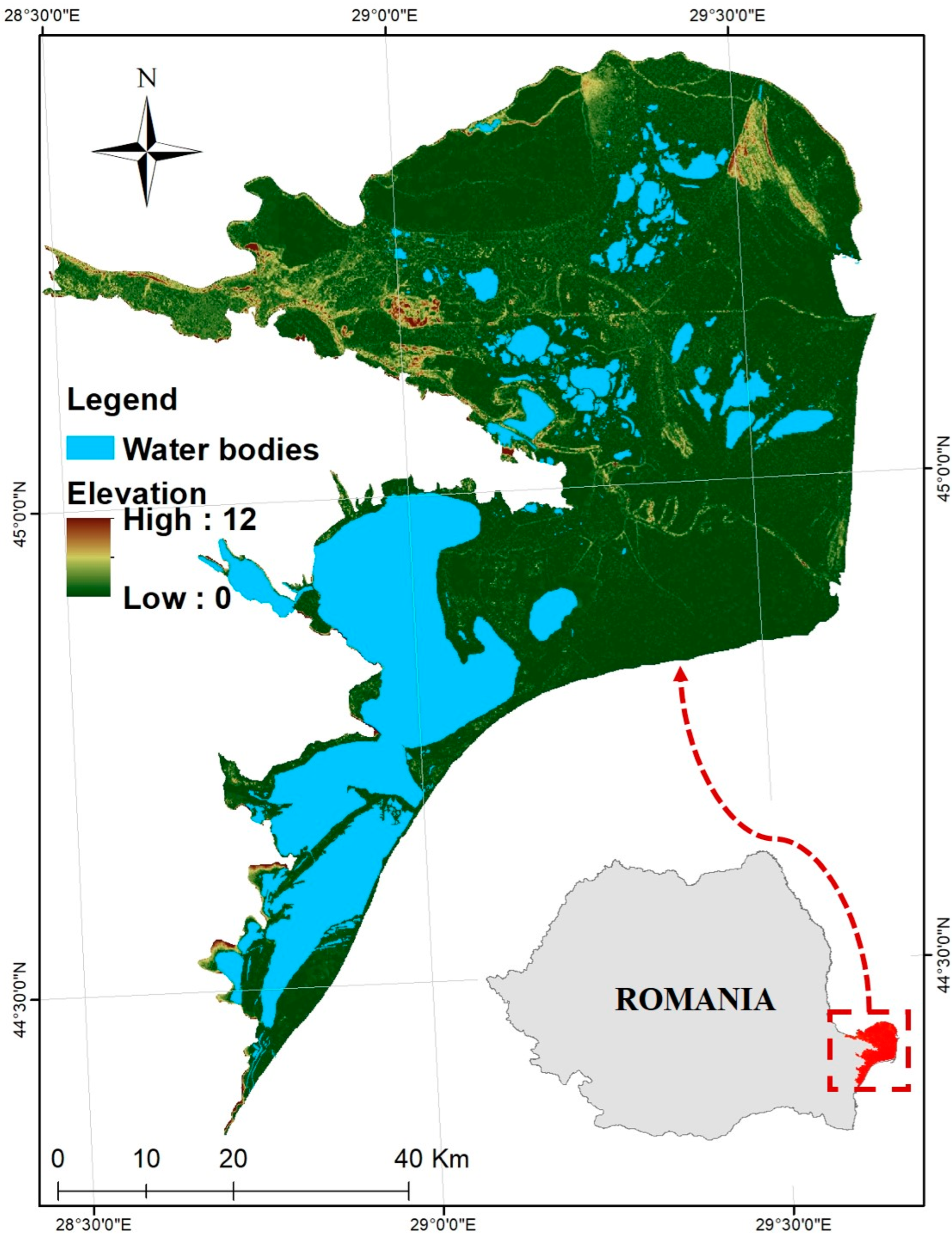
2. Study Area
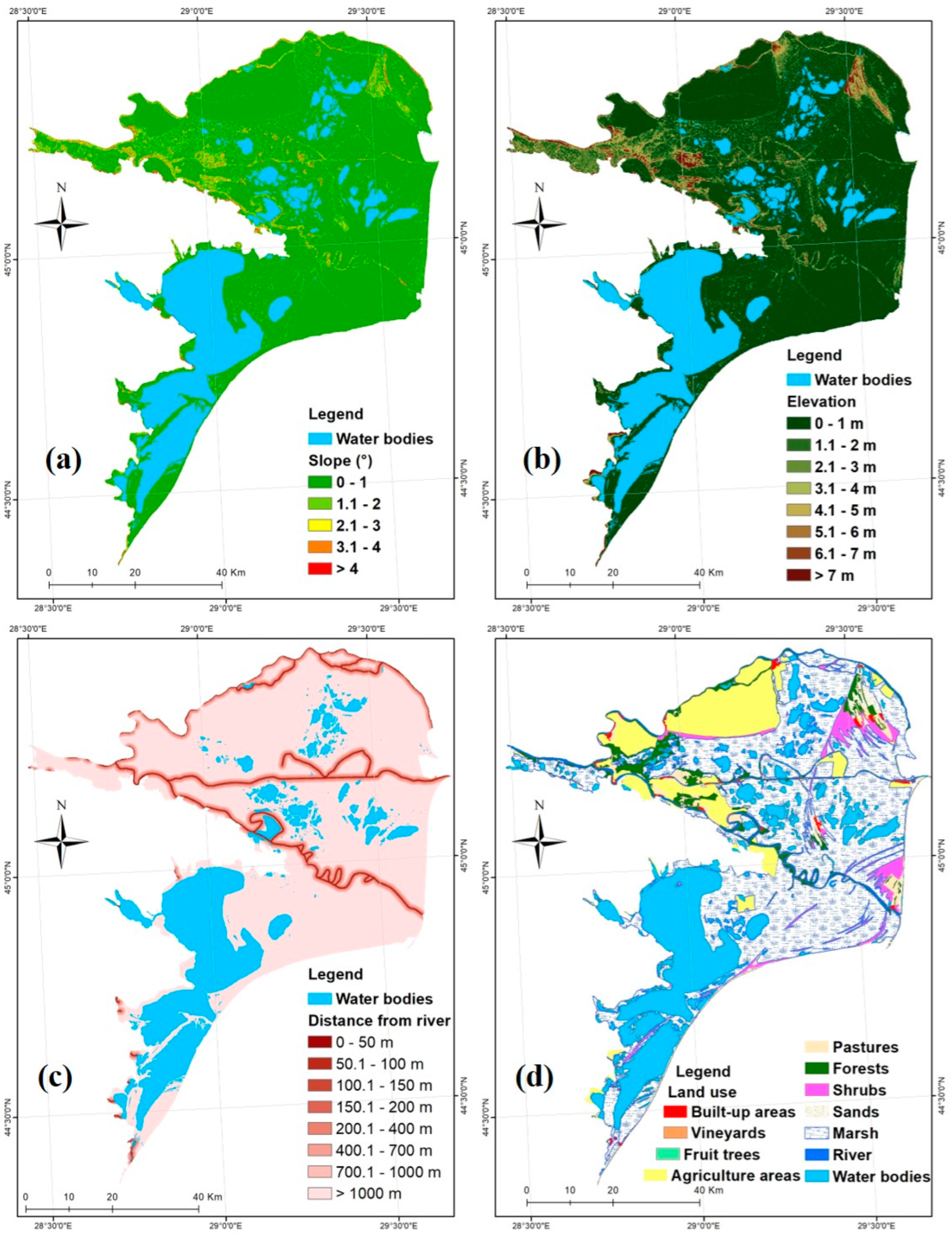
3. Data
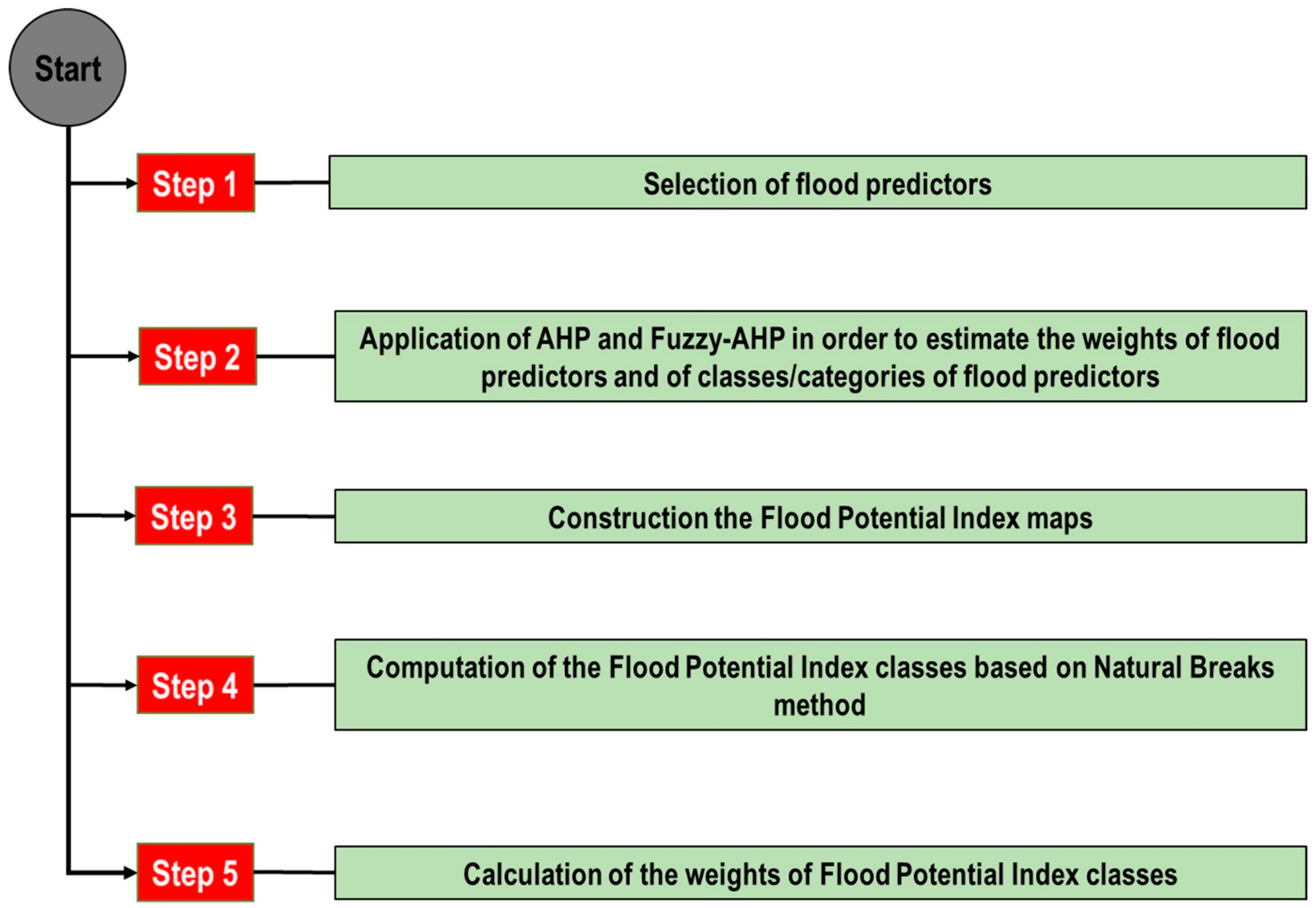
4. Methods
- (i)
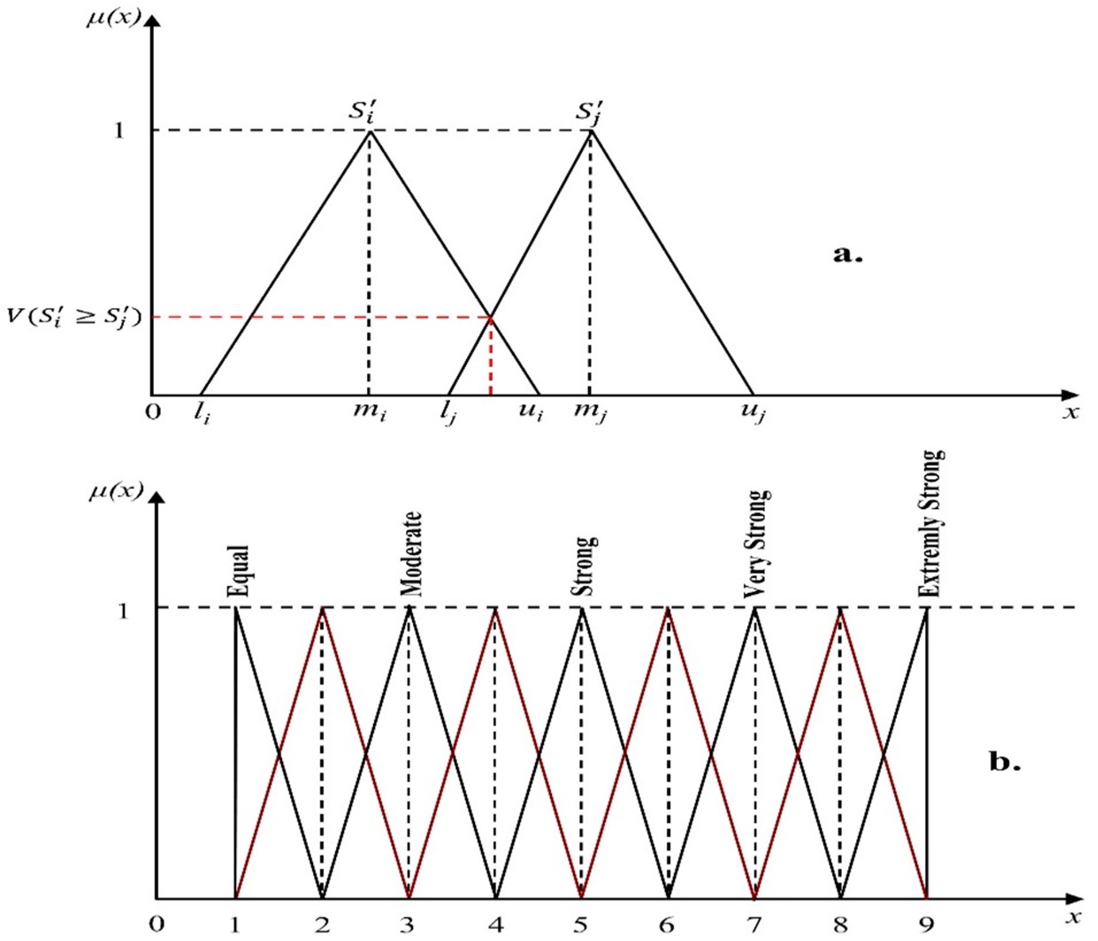
- During the construction of the pairwise comparison matrices, all flood conditioning factors were taken into account. A linguistic term was assigned to the pairwise comparison so that we would be able to determine which element/criteria is more important to the individual. The following linguistic terms were assigned:where a′ij shows a pair of criteria i and j.
- (ii)
- Through the Buckley method, the weight and fuzzy geometric mean of each criterion were calculated by:and thenwhere represents the value of fuzzy comparison among the pair criterion n and criterion i, represents the value of geometric mean associated to the fuzzy comparison values for criterion i compared to each of the other criteria, and is the fuzzy weighting of the ith criterion, which can be also represented by a TFN; = (), where , , and are the lower, middle, and upper values, respectively, of the fuzzy weighting of the ith criterion.
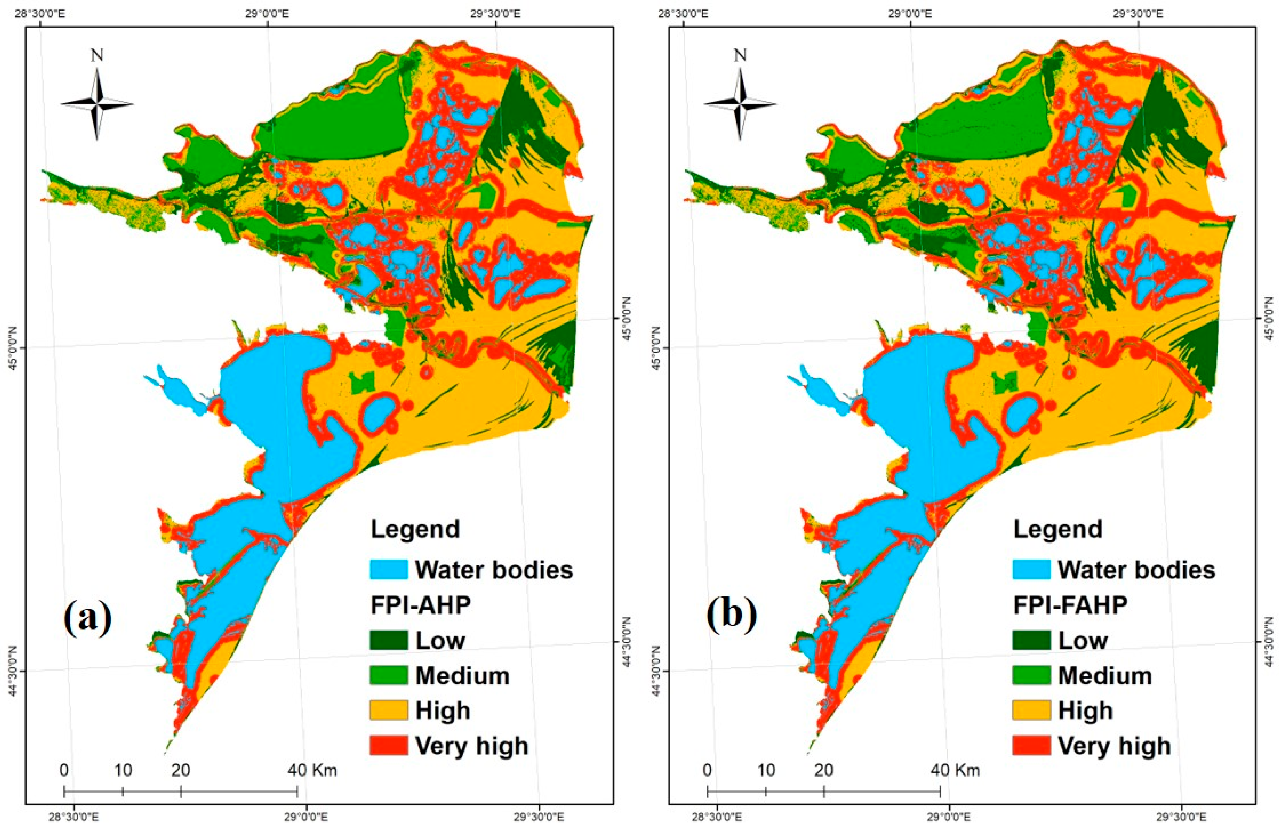
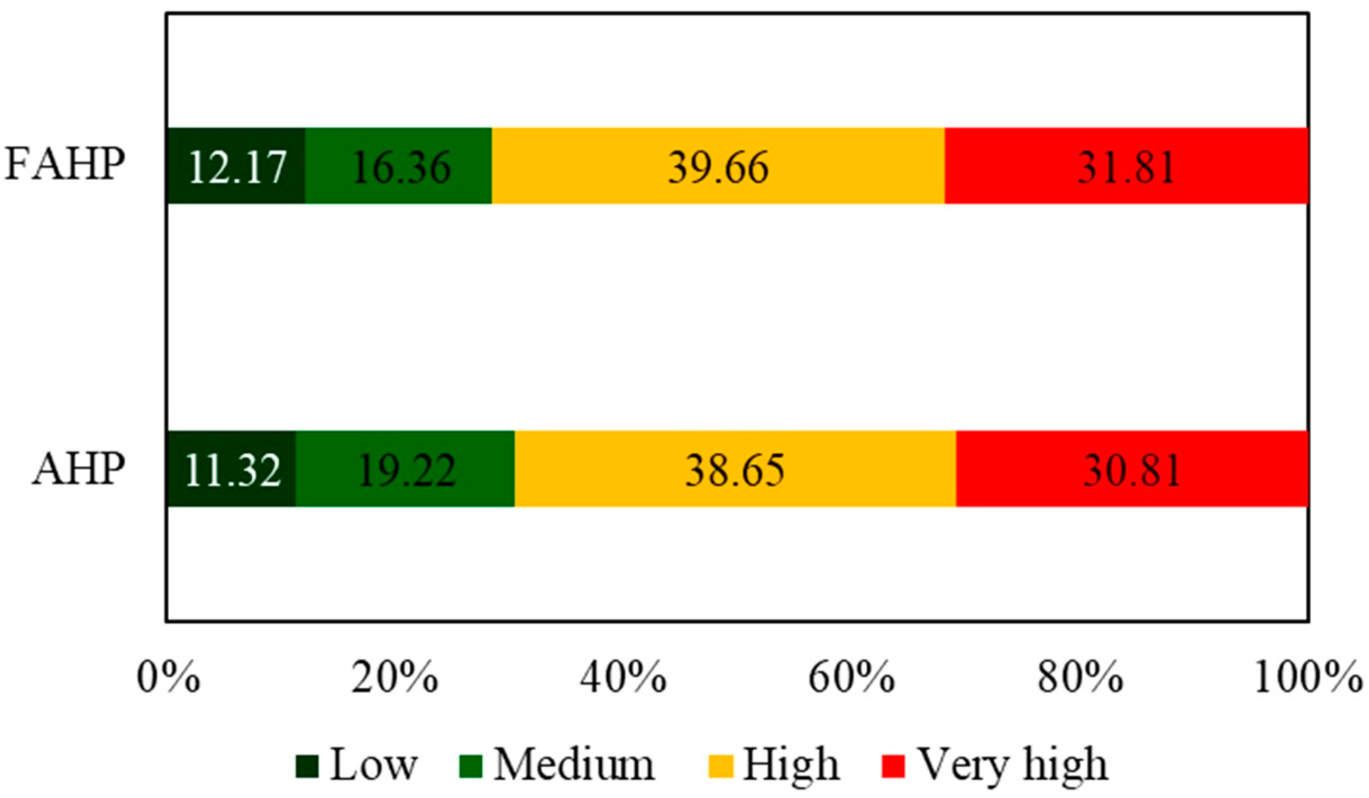
5. Results
5.1. AHP Method
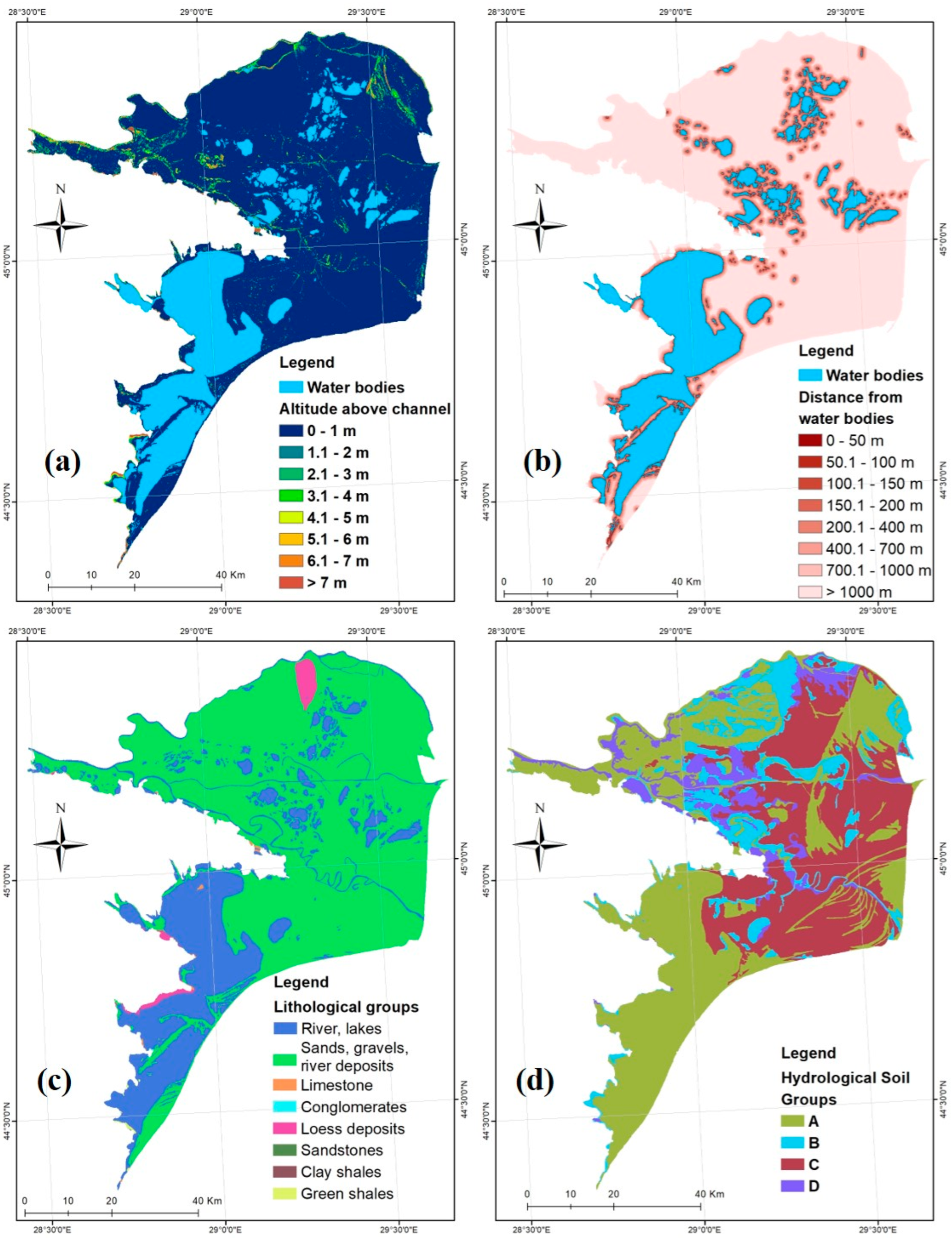
[Altitude above channel] + 0.049* [Distance from water bodies] + 0.038× [Lithology] + 0.016× [Hydrological
Soil Groups]
5.2. Fuzzy-AHP Method
0.107 × [Land use] + 0.072 × [Altitude above channel]
6. Discussion
7. Conclusions
Author Contributions
Funding
Institutional Review Board Statement
Informed Consent Statement
Data Availability Statement
Conflicts of Interest
References
- Alho, P.; Aaltonen, J. Comparing a 1D Hydraulic Model with a 2D Hydraulic Model for the Simulation of Extreme Glacial Outburst Floods. Hydrol. Process. 2008, 22, 1537–1547. [Google Scholar] [CrossRef]
- Zhang, Z.; Luo, C.; Zhao, Z. Application of probabilistic method in maximum tsunami height prediction considering stochastic seabed topography. Nat. Hazards 2020, 104, 2511–2530. [Google Scholar] [CrossRef]
- Quan, Q.; Gao, S.; Shang, Y.; Wang, B. Assessment of the sustainability of Gymnocypris eckloni habitat under river damming in the source region of the Yellow. Sci. Total Environ. 2021, 778, 146312. [Google Scholar] [CrossRef] [PubMed]
- Zhang, K.; Ali, A.; Antonarakis, A.; Moghaddam, M.; Saatchi, S.; Tabatabaeenejad, A.; Chen, R.; Jaruwatanadilok, S.; Cuenca, R.; Crow, T.W.; et al. The sensitivity of North American terrestrial carbon fluxes to spatial and temporal variation in soil moisture: An analysis using radar-derived estimates of root-zone soil moisture. J. Geophys. Res. Biogeosci. 2019, 124, 3208–3231. [Google Scholar] [CrossRef]
- Ahmadlou, M.; Karimi, M.; Alizadeh, S.; Shirzadi, A.; Parvinnejhad, D.; Shahabi, H.; Panahi, M. Flood Susceptibility Assessment Using Integration of Adaptive Network-Based Fuzzy Inference System (ANFIS) and Biogeography-Based Optimization (BBO) and BAT Algorithms (BA). Geocarto Int. 2019, 34, 1252–1272. [Google Scholar] [CrossRef]
- O’Neill, B.C.; Oppenheimer, M.; Warren, R.; Hallegatte, S.; Kopp, R.E.; Pörtner, H.O.; Scholes, R.; Birkmann, J.; Foden, W.; Licker, R. IPCC Reasons for Concern Regarding Climate Change Risks. Nat. Clim. Chang. 2017, 7, 28–37. [Google Scholar] [CrossRef]
- Jain, P.; Coogan, S.C.; Subramanian, S.G.; Crowley, M.; Taylor, S.; Flannigan, M.D. A Review of Machine Learning Applications in Wildfire Science and Management. Environ. Rev. 2020, 28, 478–505. [Google Scholar] [CrossRef]
- Zhang, K.; Wang, S.; Bao, H.; Zhao, X. Characteristics and influencing factors of rainfall-induced landslide and debris flow hazards in Shaanxi Province, China. Nat. Hazards Earth Syst. Sci. 2019, 19, 93–105. [Google Scholar] [CrossRef]
- Zhang, K.; Shalehy, M.H.; Ezaz, G.T.; Chakraborty, A.; Mohib, K.M.; Liu, L. An integrated flood risk assessment approach based on coupled hydrological-hydraulic modeling and bottom-up hazard vulnerability analysis. Environ. Model Softw. 2022, 148, 105279. [Google Scholar] [CrossRef]
- Liu, Y.; Zhang, K.; Li, Z.; Liu, Z.; Wang, J.; Huang, P. A hybrid runoff generation modelling framework based on spatial combination of three runoff generation schemes for semi-humid and semi-arid watersheds. J. Hydrol. 2020, 590, 125440. [Google Scholar] [CrossRef]
- Hong, H.; Tsangaratos, P.; Ilia, I.; Liu, J.; Zhu, A.-X.; Chen, W. Application of Fuzzy Weight of Evidence and Data Mining Techniques in Construction of Flood Susceptibility Map of Poyang County, China. Sci. Total Environ. 2018, 625, 575–588. [Google Scholar] [CrossRef] [PubMed]
- Rateb, A.; Abotalib, A.Z. Inferencing the Land Subsidence in the Nile Delta Using Sentinel-1 Satellites and GPS between 2015 and 2019. Sci. Total Environ. 2020, 729, 138868. [Google Scholar] [CrossRef] [PubMed]
- Wang, S.; Zhang, K.; Chao, L.; Li, D.; Tian, X.; Bao, H.; Chen, G.; Xia, Y. Exploring the utility of radar and satellite-sensed precipitation and their dynamic bias correction for integrated prediction of flood and landslide hazards. J. Hydrol. 2021, 603, 126964. [Google Scholar] [CrossRef]
- Asadi, H.; Shahedi, K.; Jarihani, B.; Sidle, R.C. Rainfall-Runoff Modelling Using Hydrological Connectivity Index and Artificial Neural Network Approach. Water 2019, 11, 212. [Google Scholar]
- Gao, C.; Hao, M.; Chen, J.; Gu, C. Simulation and design of joint distribution of rainfall and tide level in Wuchengxiyu Region, China. Urban Clim. 2021, 40, 101005. [Google Scholar] [CrossRef]
- Zhao, F.; Song, L.; Peng, Z.; Yang, J.; Luan, G.; Chu, C.; Ding, J.; Feng, S.; Jing, Y.; Xie, Z. Night-time light remote sensing mapping: Construction and analysis of ethnic minority development index. Remote Sens. 2021, 13, 2129. [Google Scholar] [CrossRef]
- Kim, Y.; Kimball, J.S.; Zhang, K.; Didan, K.; Velicogna, I.; McDonald, K.C. Attribution of divergent northern vegetation growth responses to lengthening non-frozen seasons using satellite optical-NIR and microwave remote sensing. Int. J. Remote Sens. 2014, 35, 3700–3721. [Google Scholar] [CrossRef]
- Chukwuma, E.; Okonkwo, C.; Ojediran, J.; Anizoba, D.; Ubah, J.; Nwachukwu, C. A GIS Based Flood Vulnerability Modelling of Anambra State Using an Integrated IVFRN-DEMATEL-ANP Model. Heliyon 2021, 7, e08048. [Google Scholar] [CrossRef]
- Chen, W.; Li, W.; Chai, H.; Hou, E.; Li, X.; Ding, X. GIS-Based Landslide Susceptibility Mapping Using Analytical Hierarchy Process (AHP) and Certainty Factor (CF) Models for the Baozhong Region of Baoji City, China. Environ. Earth Sci. 2016, 75, 63. [Google Scholar] [CrossRef]
- Pires, A.; Chang, N.-B.; Martinho, G. An AHP-Based Fuzzy Interval TOPSIS Assessment for Sustainable Expansion of the Solid Waste Management System in Setúbal Peninsula, Portugal. Resour. Conserv. Recy. 2011, 56, 7–21. [Google Scholar] [CrossRef]
- Armaş, I.; Avram, E. Perception of Flood Risk in Danube Delta, Romania. Nat. Hazards 2009, 50, 269–287. [Google Scholar] [CrossRef]
- Zhou, G.; Song, B.; Liang, P.; Xu, J.; Yue, T. Voids Filling of DEM with Multiattention Generative Adversarial Network Model. Remote Sens. 2022, 14, 1206. [Google Scholar] [CrossRef]
- Carey, S.K.; Woo, M. Slope Runoff Processes and Flow Generation in a Subarctic, Subalpine Catchment. J. Hydrol. 2001, 253, 110–129. [Google Scholar] [CrossRef]
- Costache, R. Flood Susceptibility Assessment by Using Bivariate Statistics and Machine Learning Models-A Useful Tool for Flood Risk Management. Water Resour. Manag. 2019, 33, 3239–3256. [Google Scholar] [CrossRef]
- Costache, R.; Bao Pham, Q.; Corodescu-Roșca, E.; Cîmpianu, C.; Hong, H.; Thi Thuy Linh, N.; Ming Fai, C.; Najah Ahmed, A.; Vojtek, M.; Muhammed Pandhiani, S. Using GIS, Remote Sensing, and Machine Learning to Highlight the Correlation between the Land-Use/Land-Cover Changes and Flash-Flood Potential. Remote Sens. 2020, 12, 1422. [Google Scholar] [CrossRef]
- Prăvălie, R.; Costache, R. The Vulnerability of the Territorial-Administrative Units to the Hydrological Phenomena of Risk (Flash-Floods). Case Study: The Subcarpathian Sector of Buzău Catchment. An. Univ. Oradea–Ser. Geogr. 2013, 23, 91–98. [Google Scholar]
- Dong, J.; Deng, R.; Quanying, Z.; Cai, J.; Ding, Y.; Li, M. Research on recognition of gas saturation in sandstone reservoir based on capture mode. Appl. Radiat. Isot. 2021, 178, 109939. [Google Scholar] [CrossRef]
- Fan, C.; Li, H.; Qin, Q.; He, S.; Zhong, C. Geological conditions and exploration potential of shale gas reservoir in Wufeng and Longmaxi Formation of southeastern Sichuan Basin, China. J. Pet. Sci. Eng. 2020, 191, 107138. [Google Scholar] [CrossRef]
- Xie, W.; Li, X.; Jian, W.; Yang, Y.; Liu, H.; Robledo, L.F.; Nie, W. A novel hybrid method for landslide susceptibility mapping-based geodetector and machine learning cluster: A case of Xiaojin county, China. ISPRS Int. J. Geo-Inf. 2021, 10, 93. [Google Scholar] [CrossRef]
- Agarwal, E.; Agarwal, R.; Garg, R.; Garg, P. Delineation of Groundwater Potential Zone: An AHP/ANP Approach. J. Earth Syst. Sci. 2013, 122, 887–898. [Google Scholar] [CrossRef]
- Costache, R.; Ali, S.A.; Parvin, F.; Pham, Q.B.; Arabameri, A.; Nguyen, H.; Crăciun, A.; Anh, D.T. Detection of Areas Prone to Flood-Induced Landslides Risk Using Certainty Factor and Its Hybridization with FAHP, XGBoost and Deep Learning Neural Network. Geocarto Int. 2021, 1–36. [Google Scholar] [CrossRef]
- Gigović, L.; Pamučar, D.; Bajić, Z.; Drobnjak, S. Application of GIS-Interval Rough AHP Methodology for Flood Hazard Mapping in Urban Areas. Water 2017, 9, 360. [Google Scholar] [CrossRef]
- Cao, Y.; Jia, H.; Xiong, J.; Cheng, W.; Li, K.; Pang, Q.; Yong, Z. Flash Flood Susceptibility Assessment Based on Geodetector, Certainty Factor, and Logistic Regression Analyses in Fujian Province, China. ISPRS Int. J. Geo-Inf. 2020, 9, 748. [Google Scholar] [CrossRef]
- Anquetin, S.; Braud, I.; Vannier, O.; Viallet, P.; Boudevillain, B.; Creutin, J.-D.; Manus, C. Sensitivity of the Hydrological Response to the Variability of Rainfall Fields and Soils for the Gard 2002 Flash-Flood Event. J. Hydrol. 2010, 394, 134–147. [Google Scholar] [CrossRef]
- Lee, G.; Jun, K.; Chung, E.-S. Group Decision-Making Approach for Flood Vulnerability Identification Using the Fuzzy VIKOR Method. Nat. Hazards Earth Syst. Sci. 2015, 15, 863–874. [Google Scholar] [CrossRef]
- Sattar, A.; Bonakdari, H.; Gharabaghi, B.; Radecki-Pawlik, A. Hydraulic Modeling and Evaluation Equations for the Incipient Motion of Sandbags for Levee Breach Closure Operations. Water 2019, 11, 279. [Google Scholar] [CrossRef]
- Mahmoud, S.H.; Gan, T.Y. Multi-Criteria Approach to Develop Flood Susceptibility Maps in Arid Regions of Middle East. J. Clean. Prod. 2018, 196, 216–229. [Google Scholar] [CrossRef]
- Xie, W.; Nie, W.; Saffari, P.; Robledo, L.F.; Descote, P.Y.; Jian, W. Landslide hazard assessment based on Bayesian optimization–support vector machine in Nanping City, China. Nat. Hazards 2021, 109, 931–948. [Google Scholar] [CrossRef]
- Costache, R.; Țîncu, R.; Elkhrachy, I.; Pham, Q.B.; Popa, M.C.; Diaconu, D.C.; Avand, M.; Costache, I.; Arabameri, A.; Bui, D.T. New Neural Fuzzy-Based Machine Learning Ensemble for Enhancing the Prediction Accuracy of Flood Susceptibility Mapping. Hydrol. Sci. J. 2020, 65, 2816–2837. [Google Scholar] [CrossRef]
- Chen, Z.; Liu, Z.; Yin, L.; Zheng, W. Statistical analysis of regional air temperature characteristics before and after dam construction. Urban Clim. 2022, 41, 101085. [Google Scholar] [CrossRef]
- Arora, A.; Pandey, M.; Siddiqui, M.A.; Hong, H.; Mishra, V.N. Spatial Flood Susceptibility Prediction in Middle Ganga Plain: Comparison of Frequency Ratio and Shannon’s Entropy Models. Geocarto Int. 2019, 36, 1–32. [Google Scholar] [CrossRef]
- Azareh, A.; Rafiei Sardooi, E.; Choubin, B.; Barkhori, S.; Shahdadi, A.; Adamowski, J.; Shamshirband, S. Incorporating Multi-Criteria Decision-Making and Fuzzy-Value Functions for Flood Susceptibility Assessment. Geocarto Int. 2019, 36, 1–21. [Google Scholar] [CrossRef]
- Bui, D.T.; Tsangaratos, P.; Ngo, P.-T.T.; Pham, T.D.; Pham, B.T. Flash Flood Susceptibility Modeling Using an Optimized Fuzzy Rule Based Feature Selection Technique and Tree Based Ensemble Methods. Sci. Total Environ. 2019, 668, 1038–1054. [Google Scholar] [CrossRef] [PubMed]
- Huang, Y.; Bárdossy, A.; Zhang, K. Sensitivity of hydrological models to temporal and spatial resolutions of rainfall data. Hydrol. Earth Syst. Sci. 2019, 23, 2647–2663. [Google Scholar] [CrossRef]
- Ali, S.A.; Parvin, F.; Pham, Q.B.; Vojtek, M.; Vojteková, J.; Costache, R.; Linh, N.T.T.; Nguyen, H.Q.; Ahmad, A.; Ghorbani, M.A. GIS-Based Comparative Assessment of Flood Susceptibility Mapping Using Hybrid Multi-Criteria Decision-Making Approach, Naïve Bayes Tree, Bivariate Statistics and Logistic Regression: A Case of Topľa Basin, Slovakia. Ecol. Indic. 2020, 117, 106620. [Google Scholar] [CrossRef]
- Bronstert, A. Floods and Climate Change: Interactions and Impacts. Risk Anal. 2003, 23, 545–557. [Google Scholar] [CrossRef]
- Chapi, K.; Singh, V.P.; Shirzadi, A.; Shahabi, H.; Bui, D.T.; Pham, B.T.; Khosravi, K. A Novel Hybrid Artificial Intelligence Approach for Flood Susceptibility Assessment. Environ. Model. Softw. 2017, 95, 229–245. [Google Scholar] [CrossRef]
- Yin, L.; Wang, L.; Keim, B.D.; Konsoer, K.; Zheng, W. Wavelet analysis of dam injection and discharge in three gorges dam and reservoir with precipitation and river discharge. Water 2022, 14, 567. [Google Scholar] [CrossRef]
- Yan, J.; Jiao, H.; Pu, W.; Shi, C.; Dai, J.; Liu, H. Radar Sensor Network Resource Allocation for Fused Target Tracking: A Brief Review. Inf. Fusion 2022, 87–88, 105–115. [Google Scholar] [CrossRef]


| Factors/Classes Categories | Pairwise Comparison | AHP Weights | |||||||
|---|---|---|---|---|---|---|---|---|---|
| [1] | [2] | [3] | [4] | [5] | [6] | [7] | [8] | ||
| Factors | |||||||||
| [1] Slope | 1 | 2 | 2 | 3 | 5 | 6 | 7 | 9 | 0.288 |
| [2] Elevation | 1/2 | 1 | 2 | 3 | 5 | 6 | 7 | 9 | 0.239 |
| [3] Distance from river | 1/2 | 1/2 | 1 | 2 | 4 | 5 | 6 | 9 | 0.177 |
| [4] Land use | 1/3 | 1/3 | 1/2 | 1 | 3 | 4 | 5 | 8 | 0.124 |
| [5] Altitude above channel | 1/5 | 1/5 | 1/4 | 1/3 | 1 | 2 | 3 | 7 | 0.068 |
| [6] Distance from water bodies | 1/6 | 1/6 | 1/5 | 1/4 | 1/2 | 1 | 2 | 6 | 0.049 |
| [7] Lithology | 1/7 | 1/7 | 1/6 | 1/5 | 1/3 | 1/2 | 1 | 6 | 0.038 |
| [8] Hydrological Soil Groups | 1/9 | 1/9 | 1/9 | 1/8 | 1/7 | 1/6 | 1/6 | 1 | 0.016 |
| Class/categories | |||||||||
| Slope (°) | |||||||||
| [1] 0–1 | 1 | 4 | 6 | 7 | 9 | 0.546 | |||
| [2] 1–2 | 1/4 | 1 | 3 | 4 | 6 | 0.229 | |||
| [3] 2–3 | 1/6 | 1/3 | 1 | 2 | 4 | 0.113 | |||
| [4] 3–4 | 1/7 | 1/4 | 1/2 | 1 | 3 | 0.075 | |||
| [5] >4 | 1/9 | 1/6 | 1/4 | 1/3 | 1 | 0.037 | |||
| Altitude (m) | |||||||||
| [1] 0–1 | 1 | 2 | 3 | 4 | 5 | 6 | 7 | 8 | 0.327 |
| [2] 1–2 | 1/2 | 1 | 2 | 3 | 4 | 5 | 6 | 7 | 0.227 |
| [3] 2–3 | 1/3 | 1/2 | 1 | 2 | 3 | 4 | 5 | 6 | 0.157 |
| [4] 3–4 | 1/4 | 1/3 | 1/2 | 1 | 2 | 3 | 4 | 5 | 0.108 |
| [5] 4–5 | 1/5 | 1/4 | 1/3 | 1/2 | 1 | 2 | 3 | 4 | 0.073 |
| [6] 4–6 | 1/6 | 1/5 | 1/4 | 1/3 | 1/2 | 1 | 2 | 3 | 0.050 |
| [7] 6–7 | 1/7 | 1/6 | 1/5 | 1/4 | 1/3 | 1/2 | 1 | 2 | 0.034 |
| [8] >7 | 1/8 | 1/7 | 1/6 | 1/5 | 1/4 | 1/3 | 1/2 | 1 | 0.024 |
| Distance from the river (m) | |||||||||
| [1] 0–50 | 1 | 2 | 3 | 4 | 5 | 6 | 7 | 9 | 0.323 |
| [2] 50–100 | 1/2 | 1 | 2 | 3 | 4 | 5 | 6 | 7 | 0.221 |
| [3] 100–150 | 1/3 | 1/2 | 1 | 2 | 3 | 4 | 5 | 6 | 0.152 |
| [4] 150–200 | 1/4 | 1/3 | 1/2 | 1 | 2 | 3 | 4 | 5 | 0.104 |
| [5] 200–400 | 1/5 | 1/4 | 1/3 | 1/2 | 1 | 3 | 3 | 3 | 0.073 |
| [6] 400–700 | 1/6 | 1/5 | 1/4 | 1/3 | 1/3 | 1 | 4 | 6 | 0.063 |
| [7] 700–1000 | 1/7 | 1/6 | 1/5 | 1/4 | 1/3 | 1/4 | 1 | 6 | 0.043 |
| [8] >1000 | 1/9 | 1/7 | 1/6 | 1/5 | 1/3 | 1/6 | 1/6 | 1 | 0.021 |
| Land use | |||||||||
| [1] Forests, sands | 1 | 1/3 | 1/5 | 1/7 | 1/9 | 0.035 | |||
| [2] Vineyards, fruit trees, shrubs | 3 | 1 | 1/3 | 1/5 | 1/7 | 0.069 | |||
| [3] Agriculture areas | 5 | 3 | 1 | 1/3 | 1/5 | 0.136 | |||
| [4] Pastures | 7 | 5 | 3 | 1 | 1/2 | 0.286 | |||
| [5] Built-up areas, marsh, river, water bodies | 9 | 7 | 5 | 2 | 1 | 0.474 | |||
| Altitude above channel (m) | |||||||||
| [1] 0–1 | 1 | 2 | 3 | 4 | 5 | 6 | 7 | 8 | 0.327 |
| [2] 1–2 | 1/2 | 1 | 2 | 3 | 4 | 5 | 6 | 7 | 0.227 |
| [3] 2–3 | 1/3 | 1/2 | 1 | 2 | 3 | 4 | 5 | 6 | 0.157 |
| [4] 3–4 | 1/4 | 1/3 | 1/2 | 1 | 2 | 3 | 4 | 5 | 0.108 |
| [5] 4–5 | 1/5 | 1/4 | 1/3 | 1/2 | 1 | 2 | 3 | 4 | 0.073 |
| [6] 4–6 | 1/6 | 1/5 | 1/4 | 1/3 | 1/2 | 1 | 2 | 3 | 0.050 |
| [7] 6–7 | 1/7 | 1/6 | 1/5 | 1/4 | 1/3 | 1/2 | 1 | 2 | 0.034 |
| [8] >7 | 1/8 | 1/7 | 1/6 | 1/5 | 1/4 | 1/3 | 1/2 | 1 | 0.024 |
| Distance from water bodies (m) | |||||||||
| [1] 0–50 | 1 | 2 | 3 | 4 | 5 | 6 | 8 | 9 | 0.324 |
| [2] 50–100 | 1/2 | 1 | 2 | 3 | 4 | 5 | 7 | 8 | 0.225 |
| [3] 100–150 | 1/3 | 1/2 | 1 | 2 | 3 | 4 | 6 | 7 | 0.156 |
| [4] 150–200 | 1/4 | 1/3 | 1/2 | 1 | 2 | 4 | 5 | 6 | 0.113 |
| [5] 200–400 | 1/5 | 1/4 | 1/3 | 1/2 | 1 | 2 | 3 | 4 | 0.069 |
| [6] 400–700 | 1/6 | 1/5 | 1/4 | 1/4 | 1/2 | 1 | 2 | 6 | 0.053 |
| [7] 700–1000 | 1/8 | 1/7 | 1/6 | 1/5 | 1/3 | 1/2 | 1 | 6 | 0.040 |
| [8] >1000 | 1/9 | 1/8 | 1/7 | 1/6 | 1/4 | 1/6 | 1/6 | 1 | 0.019 |
| Lithology | |||||||||
| [1] Sands, gravels, river deposits | 1 | 1/2 | 1/4 | 1/6 | 1/9 | 0.043 | |||
| [2] Loess deposits | 2 | 1 | 1/2 | 1/3 | 1/4 | 0.090 | |||
| [3] Limestone, conglomerates | 4 | 2 | 1 | 1/2 | 1/5 | 0.142 | |||
| [4] Clay shale, green shale | 6 | 3 | 2 | 1 | 1/2 | 0.256 | |||
| [5] Sandstone | 9 | 4 | 5 | 2 | 1 | 0.469 | |||
| Hydrological Soil Groups | |||||||||
| [1] A | 1 | 3/4 | 1/2 | 1/5 | 0.108 | ||||
| [2] B | 4/3 | 1 | 3/4 | 1/3 | 0.157 | ||||
| [3] C | 2 | 4/3 | 1 | 1/3 | 0.201 | ||||
| [4] D | 5 | 3 | 3 | 1 | 0.534 | ||||
| Factors | No. of Factors/Classes | λmax | CI | RI | CR |
|---|---|---|---|---|---|
| All factors | 8 | 8.067 | 0.010 | 1.41 | 0.007 |
| Slope | 5 | 5.223 | 0.056 | 1.12 | 0.050 |
| Elevation | 8 | 8.048 | 0.007 | 1.41 | 0.005 |
| Distance from river | 8 | 8.351 | 0.050 | 1.41 | 0.036 |
| Land use | 5 | 5.223 | 0.056 | 1.12 | 0.050 |
| Altitude above channel | 8 | 8.048 | 0.007 | 1.41 | 0.005 |
| Distance from water bodies | 8 | 8.351 | 0.050 | 1.41 | 0.036 |
| Lithology | 5 | 5.223 | 0.056 | 1.12 | 0.050 |
| Hydrological Soil Groups | 4 | 4.011 | 0.004 | 0.9 | 0.004 |
| 1 | 2 | 3 | 4 | 5 | 6 | 7 | 8 | |
|---|---|---|---|---|---|---|---|---|
| Slope (1) | ||||||||
| l1 | 1 | 1 | 2 | 3 | 3 | 4 | 4 | 5 |
| m1 | 1 | 2 | 3 | 4 | 4 | 5 | 5 | 6 |
| u1 | 1 | 3 | 4 | 5 | 5 | 6 | 6 | 7 |
| Elevation (2) | ||||||||
| l2 | 1/3 | 1 | 1 | 2 | 3 | 4 | 4 | 4 |
| m2 | 1/2 | 1 | 2 | 3 | 4 | 5 | 5 | 5 |
| u2 | 1 | 1 | 3 | 4 | 5 | 6 | 6 | 6 |
| Distance from river (3) | ||||||||
| l3 | 1/4 | 1/3 | 1 | 1 | 2 | 2 | 2 | 3 |
| m3 | 1/3 | 1/2 | 1 | 2 | 3 | 3 | 3 | 4 |
| u3 | 1/2 | 1 | 1 | 3 | 4 | 4 | 4 | 5 |
| Land use (4) | ||||||||
| l4 | 1/5 | 1/4 | 1/3 | 1 | 1 | 1 | 1 | 2 |
| m4 | 1/4 | 1/3 | 1/2 | 1 | 2 | 2 | 2 | 3 |
| u4 | 1/3 | 1/2 | 1 | 1 | 3 | 3 | 3 | 4 |
| Altitude above channel (5) | ||||||||
| l5 | 1/5 | 1/4 | 1/3 | 1/3 | 1 | 1 | 1 | 2 |
| m5 | 1/4 | 1/3 | 1/2 | 1/2 | 1 | 2 | 2 | 3 |
| u5 | 1/3 | 1/2 | 1 | 1 | 1 | 3 | 3 | 4 |
| Distance from water bodies (6) | ||||||||
| l6 | 1/6 | 1/5 | 1/4 | 1/3 | 1/3 | 1 | 1 | 1 |
| m6 | 1/5 | 1/4 | 1/3 | 1/2 | 1/2 | 1 | 1 | 2 |
| u6 | 1/4 | 1/3 | 1/2 | 1 | 1 | 1 | 1 | 3 |
| Lithology (7) | ||||||||
| l7 | 1/6 | 1/5 | 1/4 | 1/3 | 1/3 | 1 | 1 | 1 |
| m7 | 1/5 | 1/4 | 1/3 | 1/2 | 1/2 | 1 | 1 | 2 |
| u7 | 1/4 | 1/3 | 1/2 | 1 | 1 | 1 | 1 | 3 |
| Hydrological Soil Groups (8) | ||||||||
| l8 | 1/7 | 1/6 | 1/5 | 1/4 | 1/4 | 1/3 | 1/3 | 1 |
| m8 | 1/6 | 1/5 | 1/4 | 1/3 | 1/3 | 1/2 | 1/2 | 1 |
| u8 | 1/5 | 1/4 | 1/3 | 1/2 | 1/2 | 1 | 1 | 1 |
| Slope = 1 | Elevation = 2 | Distance from River = 3 |
| V(S1 ≥ S2) = 1 | V(S2 ≥ S1) = 1 | V(S3 ≥ S1) = 0.51 |
| V(S1 ≥ S3) = 1 | V(S2 ≥ S3) = 1 | V(S3 ≥ S2) = 0.65 |
| V(S1 ≥ S4) = 1 | V(S2 ≥ S4) = 1 | V(S3 ≥ S4) = 1 |
| V(S1 ≥ S5) = 1 | V(S2 ≥ S5) = 1 | V(S3 ≥ S5) = 1 |
| V(S1 ≥ S6) = 1 | V(S2 ≥ S6) = 1 | V(S3 ≥ S6) = 1 |
| V(S1 ≥ S7) = 1 | V(S2 ≥ S7) = 1 | V(S3 ≥ S7) = 1 |
| V(S1 ≥ S8) = 1 | V(S2 ≥ S8) = 1 | V(S3 ≥ S8) = 1 |
| min{V(S1 ≥ Sk)} = 1 | min{V(S2 ≥ Sk)} = 1 | min{V(S3 ≥ Sk)} = 0.51 |
| Weight = 0.328 | Weight = 0.328 | Weight = 0.166 |
| Land use = 4 | Altitude above channel = 5 | Distance from water bodies = 6 |
| V(S4 ≥ S1) = 0.33 | V(S5 ≥ S1) = 0.22 | V(S6 ≥ S1) = 0 |
| V(S4 ≥ S2) = 0.69 | V(S5 ≥ S2) = 0.59 | V(S6 ≥ S2) = 0 |
| V(S4 ≥ S3) = 1 | V(S5 ≥ S3) = 0.9 | V(S6 ≥ S3) = 0.17 |
| V(S4 ≥ S5) = 1 | V(S5 ≥ S4) = 1 | V(S6 ≥ S4) = 0.53 |
| V(S4 ≥ S6) = 1 | V(S5 ≥ S6) = 1 | V(S6 ≥ S5) = 0.63 |
| V(S4 ≥ S7) = 1 | V(S5 ≥ S7) = 1 | V(S6 ≥ S7) = 1 |
| V(S4 ≥ S8) = 1 | V(S5 ≥ S8) = 1 | V(S6 ≥ S8) = 1 |
| min{V(S5 ≥ Sk)} = 0.33 | min{V(S6 ≥ Sk)} = 0.22 | min{V(S7 ≥ Sk)} = 0 |
| Weight = 0.107 | >Weight = 0.072 | Weight = 0 |
| Lithology = 7 | Hydrological Soil Groups = 8 | |
| V(S7 ≥ S1) = 0 | V(S8 ≥ S1) = 0 | |
| V(S7 ≥ S2) = 0 | V(S8 ≥ S2) = 0 | |
| V(S7 ≥ S3) = 0.17 | V(S8 ≥ S3) = 0 | |
| V(S7 ≥ S4) = 0.53 | V(S8 ≥ S4) = 0.16 | |
| V(S7 ≥ S5) = 0.63 | V(S8 ≥ S5) = 0.24 | |
| V(S7 ≥ S6) = 1 | V(S8 ≥ S6) = 0.57 | |
| V(S7 ≥ S8) = 1 | V(S8 ≥ S7) = 0.57 | |
| min{V(S7 ≥ Sk)} = 0 | min{V(S8 ≥ Sk)} = 0 | |
| Weight = 0 | Weight = 0 |
Publisher’s Note: MDPI stays neutral with regard to jurisdictional claims in published maps and institutional affiliations. |
© 2022 by the authors. Licensee MDPI, Basel, Switzerland. This article is an open access article distributed under the terms and conditions of the Creative Commons Attribution (CC BY) license (https://creativecommons.org/licenses/by/4.0/).
Share and Cite
Crăciun, A.; Costache, R.; Bărbulescu, A.; Pal, S.C.; Costache, I.; Dumitriu, C.Ș. Modern Techniques for Flood Susceptibility Estimation across the Deltaic Region (Danube Delta) from the Black Sea’s Romanian Sector. J. Mar. Sci. Eng. 2022, 10, 1149. https://doi.org/10.3390/jmse10081149
Crăciun A, Costache R, Bărbulescu A, Pal SC, Costache I, Dumitriu CȘ. Modern Techniques for Flood Susceptibility Estimation across the Deltaic Region (Danube Delta) from the Black Sea’s Romanian Sector. Journal of Marine Science and Engineering. 2022; 10(8):1149. https://doi.org/10.3390/jmse10081149
Chicago/Turabian StyleCrăciun, Anca, Romulus Costache, Alina Bărbulescu, Subodh Chandra Pal, Iulia Costache, and Cristian Ștefan Dumitriu. 2022. "Modern Techniques for Flood Susceptibility Estimation across the Deltaic Region (Danube Delta) from the Black Sea’s Romanian Sector" Journal of Marine Science and Engineering 10, no. 8: 1149. https://doi.org/10.3390/jmse10081149
APA StyleCrăciun, A., Costache, R., Bărbulescu, A., Pal, S. C., Costache, I., & Dumitriu, C. Ș. (2022). Modern Techniques for Flood Susceptibility Estimation across the Deltaic Region (Danube Delta) from the Black Sea’s Romanian Sector. Journal of Marine Science and Engineering, 10(8), 1149. https://doi.org/10.3390/jmse10081149