Spectral Kinetic-Energy Fluxes in the North Pacific: Definition Comparison and Normal- and Shear-Strain Decomposition

Abstract

The spectral kinetic-energy flux is an effective tool to analyze the kinetic-energy transfer across a range of length scales, also known as the kinetic-energy cascade. Three methods to calculate spectral energy fluxes have been widely used, hereafter the Π_A, Π_F, and Π_Q definitions. However, the relations among these three definitions have not been examined in detail. Moreover, the respective contribution of the normal strain and shear strain of the flow field to kinetic-energy cascade has not been estimated before. Here, we use the kinetic energy equations to rigorously compare these definitions. Then, we evaluate the spectral energy fluxes, as well as its decomposition into the normal-strain and shear-strain components for the North Pacific, using a dynamically consistent global eddying state estimate. We find that the data must be preprocessed first to obtain stable results from the Π_F and Π_Q definitions, but not for the Π_A definition. For the upper 500 m of the North Pacific, in the wavenumber ranges with inverse kinetic-energy cascade, both the normal and shear-strain flow components contribute significantly to the spectral energy fluxes. However, at high wavenumbers, the dominant contributor to forward kinetic-energy cascade is the normal-strain component. These results should help shed light on the underlying mechanism of inverse and forward energy cascades.

1. Introduction

Due to the ocean’s intrinsic nonlinearity and turbulent nature, its energy may transfer across length scales spanning nearly ten orders of magnitude, from tens of thousands of kilometers down to millimeters. This phenomenon, called energy cascade in turbulence theory, has a great impact on the transport and redistribution of energy and key tracers in the ocean (e.g., heat, salt) [1,2]. Thus, detailed exploration of this energy cascade can help us better understand the energy balance in the ocean.

The kinetic-energy cascade, an important metric to characterize turbulence, is of great oceanographic interest. This cascade can go “forward”, from large-to-small scale, as well as “inverse”, from small-to-large. The large-scale component of oceanic motions are quasi two-dimensional due to the prevalence of stratification and the Earth’s rotation [3,4]. A remarkable feature of quasi two-dimensional turbulence is that kinetic energy is transferred from small to large scales, i.e., inverse kinetic-energy cascade occurs [5,6,7,8]. The geostrophic turbulence theory for the stratified ocean predicts that, on a scale larger than the Rossby deformation radius, the barotropic mode (which is mainly kinetic energy) undergoes an inverse cascade, whereas potential and total energy in the baroclinic mode cascade downscale. On a scale near the deformation radius, most of the energy in the baroclinic mode is transferred to the barotropic mode [6,8,9,10].

The diagnostic framework of spectral kinetic-energy fluxes proposed by Frisch [11] is an effective tool to estimate the transfer of kinetic energy between different scales. Using this tool, Scott and Wang [12] diagnosed spectral kinetic-energy fluxes induced by geostrophic motions in the South Pacific Ocean using satellite altimeter data. Their results provided direct evidence of an inverse kinetic-energy cascade in the ocean. However, the altimeter data mainly measures the first baroclinic mode in the ocean [13]. To further understand why the inverse cascade occurs in the baroclinic mode, Scott and Arbic [14] considered the problem of kinetic-energy cascade in an idealized two-layer quasi-geostrophic model. They found that kinetic energy in barotropic and baroclinic modes both undergo an inverse cascade, whereas the potential and total energy in the baroclinic mode undergo a forward cascade. More recent studies using this diagnostic tool give further observation/model evidence for the prevalence of an inverse kinetic-energy cascade in the ocean [15,16,17,18,19].

Recently, the characteristics of kinetic-energy cascade in the ocean have been widely discussed. These studies include those on the geographical variability of inverse cascades [16,18,19,20,21], the depth dependence of inverse cascades [18,21], the anisotropy of inverse cascades [18,19], and on assessing forward cascades at a small scale [22,23,24]. For example, Wang et al. [18] found that the stronger inverse cascade occurs in the region with higher eddy kinetic energy, with a strength that decreases with an increase in depth. Wang et al. [18] and Ajayi et al. [21] discussed the geographical patterns of energy injection scales and arrest scales, and found that they vary greatly with latitude, but change little with depth. Li et al. [19] focused on the anisotropy of the inverse cascade, and pointed out that a strong anisotropy may govern multiple jets in the ocean. Moreover, Brüggemann and Eden [24] explored the mechanism of the forward cascade at a small scale, finding it to be related to ageostrophic dynamics.

Due to the different definitions and gauge of energy transfer across scales and energy transport in space, there are many definitions of spectral kinetic-energy fluxes [20]. Although the studies summarized above all provide illuminating findings, they used various definitions of spectral kinetic-energy flux, different choices of diagnosis domain and data preprocessing methods. The inconsistent use of the spectral energy flux definition makes it difficult to consistently compare energy cascade results from different studies. It is also unclear whether differences in results arise from differences in the definition of spectral energy flux or from other factors such as differences in underlying dynamics, spatiotemporal variability, or data and model differences.

The spectral energy fluxes have been derived in three ways. The first was proposed by Frisch [11]. Briefly, low-pass filtering is applied to the momentum equation to obtain the equation of large-scale kinetic energy. Then, one focuses on a term in this energy equation that arises from advection. One can then obtain the spectral kinetic-energy flux by subtracting the large-scale advection of large-scale kinetic energy from this term. We label this definition as Π_F. Later, Capet et al. [22] and Qiu et al. [1] showed how one can derive the equation of spectral kinetic energy density by applying a Fourier transform to the momentum equation. Then, one integrates the advection term from this equation in the wavenumber domain, defining this integral as the spectral kinetic-energy flux, hereafter Π_Q. A recent definition was proposed by Aluie et al. [20]. Similar to that with the Π_F definition, one starts from a term in the large-scale kinetic energy equation that arises from advection in the original momentum equation. However, this term is divided into two parts: one is related to the spatial transport of large-scale kinetic energy, which is not the same as advection; and the other is interpreted as the transfer of kinetic energy among motions of different scales and thus is defined as the spectral kinetic-energy flux Π_A. Although Aluie et al. [20] compared the Π_F and Π_A definitions, the relation of all three has not been rigorously analyzed. To help fill this knowledge gap, one goal of this study is to compare these definitions mathematically and physically.

The diagnostic formulas of spectral kinetic-energy fluxes (Section 2) reveal that without flow strain, the spectral energy fluxes would vanish. Such a strain has both a normal-strain component and a shear-strain component. Consequently, based on the type of strain, the spectral kinetic-energy flux can be divided into two components. One component is related to the horizontal shear strain of the flow, and the other component is related to the horizontal normal strain. Their respective contributions to the total kinetic-energy cascade are unknown. The second goal of the paper is to estimate these contributions.

Although the role of normal strain and shear strain in the energy cascade has largely remained unexplored, their individual roles in the eddy-mean flow interaction have been carefully discussed [25,26,27,28,29,30,31,32]. (This eddy-mean flow interaction is essentially a special form of energy cascade.) For example, Qiao and Weisberg [27] found that both components of the eddy-mean flow interaction play an important role in the generation and maintenance of instability waves. Holmes and Thomas [29] found that the shear-strain component is the main driving factor of kinetic energy in tropical instability waves, and the normal-strain component plays an important role in the initial change in kinetic energy of tropical instability waves. Such studies motivated us to examine the respective contributions of horizontal normal-strain and shear-strain components to the kinetic-energy cascade. This decomposition can probably help further reveal the underlying kinematic mechanism of inverse and forward energy cascade.

To summarize, the goals of this paper are (1) to compare the three definitions of spectral kinetic-energy flux and evaluate their diagnostic performance, and (2) to decompose the spectral kinetic-energy flux into the horizontal normal- and shear-strain components, and discuss their respective contributions to kinetic-energy cascade. For this study, we use the Estimating the Circulation and Climate of the Ocean, phase 2 (ECCO2), high-resolution global-ocean and sea-ice data synthesis state estimate. ECCO2 is dynamically consistent and appropriate for energy budget diagnosis [33,34], with many studies finding it useful for examining the eddy and kinetic-energy cascade [18,19,34,35,36].

This paper is organized as follows. Section 2 presents the definition of spectral kinetic-energy flux, data source, and processing method. Section 3 presents the main results, including the comparison of different definitions of spectral flux, and the respective contributions of normal strain and shear strain to the characteristics of kinetic-energy cascade. Section 4 summarizes the main conclusions.

2. Diagnostic Methods and Model

2.1. Definition of Spectral Kinetic-Energy Flux

All three definitions of spectral kinetic-energy fluxes start from the advection term of the momentum equation and thus arise from nonlinearity of the fluid system. These fluxes represent the energy transfer among motions of different scales, rather than the sources or sinks of kinetic energy [1,2]. It is thus an effective tool for diagnosing kinetic-energy cascade. This section describes the three widely used definitions of spectral kinetic-energy flux.

2.1.1. Definition I: Π_Q

This definition, hereafter “Definition I”, of the spectral kinetic-energy flux (Π_Q) refers to that used in Capet et al. [22] and Qiu et al. [1]. In this case, terms of the momentum equation are Fourier transformed to obtain the kinetic energy budget equation in the wavenumber domain. In this domain, the integral of the advection term is defined as the spectral kinetic-energy flux. It has been widely used in studies of the kinetic-energy cascade [18,19,21,37,38,39,40].

Definition I starts from the horizontal momentum equations in Cartesian coordinates on a rotating Earth:

$$\frac{\partial u}{\partial t}+u\frac{\partial u}{\partial x}+v\frac{\partial u}{\partial y}-fv=-\frac{1}{\rho }\frac{\partial p}{\partial x}+F{r}^x,$$

(1)

$$\frac{\partial v}{\partial t}+u\frac{\partial v}{\partial x}+v\frac{\partial v}{\partial y}+fu=-\frac{1}{\rho }\frac{\partial p}{\partial y}+F{r}^y,$$

(2)

where u and v are the zonal and meridional velocities, f is the Coriolis parameter, p is the pressure, and ρ is density. The Fr^x and Fr^y terms represent friction and the vertical advection of momentum. Now, take the discrete Fourier transform (DFT) of Equations (1) and (2), and run the following operations: $\mathcal{F}{(u)}^{\ast }\times \mathcal{F}[\mathrm{Equation}(1)]+\mathcal{F}(u)\times \mathcal{F}{[\mathrm{Equation}(1)]}^{\ast }+\mathcal{F}{(v)}^{\ast }\times \mathcal{F}[\mathrm{Equation}(2)]+\mathcal{F}(v)\times \mathcal{F}{[\mathrm{Equation}(2)]}^{\ast }$, where $\mathcal{F}$ represent the DFT operation and * indicates complex conjugate. With the result, one can obtain the budget equation of spectral kinetic energy density E (k_x,k_y,t)

$$\frac{\partial E(k_x,k_y,t)}{\partial t}=T(k_x,k_y,t)+P(k_x,k_y,t)-D(k_x,k_y,t),$$

(3)

when E (k_x,k_y,t) is defined as

$$E(k_x,k_y,t)=\frac{1}{2}[\mathcal{F}{(u)}^{\ast }\mathcal{F}(u)+\mathcal{F}{(v)}^{\ast }\mathcal{F}(v)]/\Delta k^2.$$

(4)

Here, ∆k² = 1/(L_xL_y), with L_x and L_y being the sizes of the selected region in the zonal and meridional directions. Thus, L_x = N_x∆x, L_y = N_y∆y, with ∆x and N_x being the grid spacing and number of grid points in the zonal direction, ∆y and N_y being those for meridional. The horizontal wavenumber vector is defined as (k_x, k_y) = 2π (m/L_x, n/L_y), where m $\in$ [−N_x/2, N_x/2], n $\in$ [−N_y/2, N_y/2]. In Equation (3), P (k_x,k_y,t) is the forcing term, including the conversion rate of available potential energy to kinetic energy. The dissipation term D (k_x,k_y,t) is derived from the Fr^x and Fr^y terms in Equations (1) and (2). The T (k_x,k_y,t) term, originating from the advection term in the momentum equation, is used to measure the redistribution of kinetic energy among different spatial scales,

$$T(k_x,k_y,t)=-\Re [\mathcal{F}{(u)}^{\ast }\mathcal{F}(u\frac{\partial u}{\partial x}+v\frac{\partial u}{\partial y})+\mathcal{F}{(v)}^{\ast }\mathcal{F}(u\frac{\partial v}{\partial x}+v\frac{\partial v}{\partial y})]/\Delta k^2,$$

(5)

where $\Re$ means the real part of the expression. We define the total wavenumber as $K=\sqrt{k_x{}^2+k_y{}^2}$, also called the isotropic wavenumber. Finally, the spectral kinetic-energy flux Π_Q is obtained by integrating T (k_x,k_y,t) from wavenumber K’ to the maximum available wavenumber

$${\prod }_Q(K^{\prime },t)={\displaystyle \sum _{K>K^{\prime }}T(k_x,k_y,t)}\Delta k^2.$$

(6)

This derivation follows that in Capet et al. [22]. To compare with other definitions of spectral energy flux (e.g., Section 3.1), we define the integration of T (k_x,k_y,t) from the minimum wavenumber to the wavenumber K’ as Π_Q,oppo,

$${\prod }_{Q,oppo}(K^{\prime },t)={\displaystyle \sum _{K<K^{\prime }}T(k_x,k_y,t)}\Delta k^2.$$

(7)

2.1.2. Definition II: Π_F

Another widely used diagnostic method of spectral energy fluxes was proposed by Frisch [11], hereafter “Definition II” [12,15,16]. Briefly, one applies low-pass filtering to the momentum equation. Then, the spectral flux Π_F is defined as the advection term in the budget equation of large-scale kinetic energy. In detail, the horizontal velocity vector u = (u, v) is expanded into the form of Fourier series,

$$u(x,y)={\displaystyle \sum _{K^{\prime }=0}^{\infty }\mathcal{F}(u)\exp i(k_{x}x+k_{y}y)}.$$

(8)

Then, the low-pass and high-pass filtered velocities are defined as

$$u_K^{<}(x,y)={\displaystyle \sum _{K^{\prime }=0}^K\mathcal{F}(u)\exp i(k_{x}x+k_{y}y)},$$

(9)

$$u_K^{>}(x,y)={\displaystyle \sum _{K^{\prime }=K}^{\infty }\mathcal{F}(\mathbf{u})\exp i(k_{x}x+k_{y}y)},$$

(10)

where the low-pass filtered velocity ${\mathbf{u}}_K^{<}=({\mathbf{u}}_K^{<},v_K^{<})$ represents the flow with spatial scales larger than 2π/K. The corresponding large-scale kinetic energy $EK{E}_K^{<}$ is defined as

$$EK{E}_K^{<}=\frac{1}{2}〈{\mathbf{u}}_K^{<}{\mathbf{u}}_K^{<}+v_K^{<}{v}_K^{<}〉,$$

(11)

where $\langle$$\rangle$ represents the spatial average on the selected region. This definition also begins with the horizontal momentum equation. By applying low-pass filtering to Equations (1) and (2), multiplying them by low-pass filtered velocities ${\mathbf{u}}_K^{<}$ and $v_K^{<}$, respectively, adding them and spatially averaging on a selected region, one obtains the budget equation of kinetic energy $EK{E}_K^{<}$:

$$\frac{\partial EK{E}_K^{<}}{\partial t}=-{\prod }_{\mathrm{total}}+F-D,$$

(12)

where the F and D terms are forcing and dissipation, respectively. The F term includes the energy transfer from available potential energy to kinetic energy through baroclinic instability. Π_total originates from the advection term in the momentum equation, which can measure the redistribution of kinetic energy among different scales. In particular,

$${\prod }_{\mathrm{total}}=〈u_K^{<}{(u\frac{\partial u}{\partial x}+v\frac{\partial u}{\partial y})}_K^{<}+v_K^{<}{(u\frac{\partial v}{\partial x}+v\frac{\partial v}{\partial y})}_K^{<}〉.$$

(13)

According to Parseval’s theorem, the low-pass filtered and high-pass filtered components are orthogonal, that is, for any real function f and g, the equation $〈f_K^{<}\cdot g_K^{>}〉=0$ holds. Then, Π_total can be simplified to

$${\prod }_{\mathrm{total}}=〈u_K^{<}(u\frac{\partial u}{\partial x}+v\frac{\partial u}{\partial y})+v_K^{<}(u\frac{\partial v}{\partial x}+v\frac{\partial v}{\partial y})〉.$$

(14)

After decomposing the horizontal velocities u and v into low- and high-pass filtered components, we divided Equation (14) into four terms:

$$\begin{array}{cc}\hfill & {\prod }_{\mathrm{total}}=〈u_K^{<}{u}_K^{<}\frac{\partial u_K^{>}}{\partial x}+u_K^{<}{v}_K^{<}\frac{\partial u_K^{>}}{\partial y}+v_K^{<}{u}_K^{<}\frac{\partial v_K^{>}}{\partial x}+v_K^{<}{v}_K^{<}\frac{\partial v_K^{>}}{\partial y}〉+〈u_K^{<}{u}_K^{>}\frac{\partial u_K^{>}}{\partial x}+u_K^{<}{v}_K^{>}\frac{\partial u_K^{>}}{\partial y}+v_K^{<}{u}_K^{>}\frac{\partial v_K^{>}}{\partial x}+v_K^{<}{v}_K^{>}\frac{\partial v_K^{>}}{\partial y}〉\hfill \\ \hfill & +\underset{{\prod }_{\mathrm{total},\mathrm{III}}}{\underbrace{〈u_K^{<}{u}_K^{<}\frac{\partial u_K^{<}}{\partial x}+u_K^{<}{v}_K^{<}\frac{\partial u_K^{<}}{\partial y}+v_K^{<}{u}_K^{<}\frac{\partial v_K^{<}}{\partial x}+v_K^{<}{v}_K^{<}\frac{\partial v_K^{<}}{\partial y}〉}}+\underset{{\prod }_{\mathrm{total},\mathrm{IV}}}{\underbrace{〈u_K^{<}{u}_K^{>}\frac{\partial u_K^{<}}{\partial x}+u_K^{<}{v}_K^{>}\frac{\partial u_K^{<}}{\partial y}+v_K^{<}{u}_K^{>}\frac{\partial v_K^{<}}{\partial x}+v_K^{<}{v}_K^{>}\frac{\partial v_K^{<}}{\partial y}〉}}.\hfill \end{array}$$

(15)

Frisch [11] assumed that the advection of low-pass filtered horizontal velocity ${\mathit{u}}_K^{<}$ with horizontal velocity u has no effect on $EK{E}_K^{<}$ budget. Therefore, the third and fourth terms Π_total,III and Π_total,IV are not included as part of the spectral kinetic-energy fluxes. The spectral flux on any wavenumber K is defined as Π_F:

$${\prod }_F=〈u_K^{<}u\frac{\partial u_K^{>}}{\partial x}+u_K^{<}v\frac{\partial u_K^{>}}{\partial y}+v_K^{<}u\frac{\partial v_K^{>}}{\partial x}+v_K^{<}v\frac{\partial v_K^{>}}{\partial y}〉.$$

(16)

The definition of Π_total above, based on velocities, is essentially the same with the spectral kinetic-energy flux in Table 5.2 of Chen [41], which is based on the streamfunction. (This consistency can be proved using the relation between streamfunction and velocity. In Chen [41], the definition of Π_total is used to assess the energy cascade in an idealized doubly periodic domain, and thus the third and fourth terms in Equation (15) above are zero.)

2.1.3. Definition III: Π_A

“Definition III” is from Aluie et al. [20]. The derivation of the large-scale kinetic energy equation in this case is similar to that in definition II, except that this derivation assumes a two-dimensional incompressible fluid and divides the energy term arising from momentum advection into two parts. The part related to the spatial transport of large-scale kinetic energy acts to spatially redistribute kinetic energy and thus is not included as part of the spectral kinetic-energy flux. The part representing the transfer of kinetic energy among different scales is defined as the spectral kinetic-energy flux.

Consistent with the previous two definitions, definition III is also derived from the horizontal momentum equation. However, it assumes that the fluid is two-dimensional and incompressible, that is, $\partial u/\partial x+\partial v/\partial y=0$. Equations (1) and (2) are rewritten as

$$\frac{\partial u}{\partial t}+\frac{\partial (uu)}{\partial x}+\frac{\partial (uv)}{\partial y}-fv=-\frac{1}{\rho }\frac{\partial p}{\partial x}+F{r}^x,$$

(17)

$$\frac{\partial v}{\partial t}+\frac{\partial (uv)}{\partial x}+\frac{\partial (vv)}{\partial y}+fu=-\frac{1}{\rho }\frac{\partial p}{\partial y}+F{r}^y.$$

(18)

Similarly, applying low-pass filtering to Equations (17) and (18), and dividing the second and third terms on the left side into two parts gives

$$\frac{\partial u_K^{<}}{\partial t}+u_K^{<}\frac{\partial u_K^{<}}{\partial x}+v_K^{<}\frac{\partial u_K^{<}}{\partial y}-f{v}_K^{<}=-\frac{\partial }{\partial x}[{(uu)}_K^{<}-u_K^{<}{u}_K^{<}]-\frac{\partial }{\partial y}[{(uv)}_K^{<}-u_K^{<}{v}_K^{<}]-\frac{1}{\rho }\frac{\partial p_K^{<}}{\partial x}+{(F{r}^x)}_K^{<},$$

(19)

$$\frac{\partial v_K^{<}}{\partial t}+u_K^{<}\frac{\partial v_K^{<}}{\partial x}+v_K^{<}\frac{\partial v_K^{<}}{\partial y}+f{u}_K^{<}=-\frac{\partial }{\partial x}[{(uv)}_K^{<}-u_K^{<}{v}_K^{<}]-\frac{\partial }{\partial y}[{(vv)}_K^{<}-v_K^{<}{v}_K^{<}]-\frac{1}{\rho }\frac{\partial p_K^{<}}{\partial y}+{(F{r}^y)}_K^{<}.$$

(20)

Then, multiply Equations (19) and (20) by the low-pass filtered velocities $u_K^{<}$ and $v_K^{<}$, respectively, sum them, and spatially average over the selected region to obtain the budget equation of large-scale kinetic energy $EK{E}_K^{<}$:

$$\frac{\partial EK{E}_K^{<}}{\partial t}+J={\prod }_A+F-D,$$

(21)

where,

$${\prod }_A=[{(uu)}_K^{<}-u_K^{<}{u}_K^{<}]\frac{\partial u_K^{<}}{\partial x}+[{(uv)}_K^{<}-u_K^{<}{v}_K^{<}]\frac{\partial u_K^{<}}{\partial y}+[{(uv)}_K^{<}-u_K^{<}{v}_K^{<}]\frac{\partial v_K^{<}}{\partial x}+[{(vv)}_K^{<}-v_K^{<}{v}_K^{<}]\frac{\partial v_K^{<}}{\partial y},$$

(22)

$$\begin{array}{ll}J=& \stackrel{J_1}{\overbrace{\frac{\partial }{\partial x}(u_K^{<}\cdot EK{E}_K^{<})+\frac{\partial }{\partial y}(v_K^{<}\cdot EK{E}_K^{<})}}\\ & +\underset{J_2}{\underbrace{\frac{\partial }{\partial x}\{u_K^{<}[{(uu)}_K^{<}-u_K^{<}{u}_K^{<}]+v_K^{<}[{(uv)}_K^{<}-u_K^{<}{v}_K^{<}]\}+\frac{\partial }{\partial y}\{u_K^{<}[{(uv)}_K^{<}-u_K^{<}{v}_K^{<}]+v_K^{<}[{(vv)}_K^{<}-v_K^{<}{v}_K^{<}]\}}},\end{array}$$

(23)

with Π_A being the spectral kinetic-energy flux at any wavenumber K, and J is related to the spatial transport of large-scale kinetic energy. Comparing the kinetic energy equations in definitions II and III, note that Π_total in Equation (12) is divided into Π_A and J in Equation (21). Definition III not only separates energy transfer across scales from spatial energy transport, but also satisfies Galilean invariance, that is, the value of spectral flux at any point does not depend on the observer’s velocity [20]. For example, when an arbitrary constant velocity U₀ is added to the original flow field u into Equation (22), the result is the same. Therefore, definition III is negligibly affected by the background flow.

Physically, the above three definitions of spectral kinetic-energy flux are all intended to represent the transfer of kinetic energy between length scales. A positive flux indicates a forward cascade, that is, kinetic energy transfer from larger to smaller scale, a negative flux is instead an inverse cascade. According to the budget equation of spectral kinetic energy density or spectral kinetic energy (i.e., Equations (3), (12) and (21)), for a statistical steady state after long-time mean, $\partial EK{E}_K^{<}/\partial t$ approaches zero. A positive slope of flux indicates that the forcing term exceeds the dissipation term, making this scale a source of kinetic energy in the long-time mean. The opposite holds for a negative slope.

2.2. Model Solution: ECCO2 State Estimate

Here, we diagnose the spectral kinetic-energy fluxes from Section 2.1 using the ECCO2 state estimate. The ECCO2 simulation is based on the Massachusetts Institute of Technology ocean general circulation model and a series of available satellite and in situ data [42,43]. The model employs cube-sphere grid projection, with a mean horizontal resolution of 18 km. Therefore, it can effectively resolve large-scale and mesoscale motions at mid- and low latitudes in the ocean. It has 50 vertical layers, with layer thickness ranging from 10 to 456 m. The model uses quadratic drag coefficients to parameterize ocean bottom processes and biharmonic horizontal viscosity for the parameterization of friction. The K-profile parameterization (KPP) mixing scheme is used to subgrid-scale parameterize the vertical mixing process [44].

The state estimation method used in the Cube 92 version of ECCO2 is the Green’s function approach. The model solution is obtained by a free-forward model run with optimized control parameters. Therefore, the solution is dynamically consistent with no non-physical jump or artificial source/sink, and thus is applicable for energy budget diagnosis [33,34]. This model solution has been applied elsewhere to study the eddy and kinetic-energy cascade [18,19,34,35,36]. We analyze the data averaged every three days during the years 1992–2003, and assume the 12-year mean represents the climatological mean of the spectral flux.

2.3. Data Processing Method

Here, we describe our choice of domain size, data preprocessing method and filtering method, etc. Inspired by Scott and Wang [12], we assess the sensitivity of the estimated spectral kinetic-energy fluxes to the choice of domain size (Figure 1). Though there are slight differences of energy fluxes at low wavenumbers (e.g., the maximum magnitude of energy fluxes), the overall structure and the zero-crossing point are insensitive to the choice of domain size. Though the domain size should be large enough to capture mesoscale information, a too-large domain size would lead to results not satisfying locality. Therefore, next we mainly present results based on a domain size of 10° × 10° (40 × 40 grid points), which is close to that used in several recent studies [15,16,18,21,45].

The meridional and zonal velocities during 1992–2003 from the ECCO2 state estimate are used to calculate the spectral kinetic-energy flux. The low-pass filtering operation used here is to take the DFT of velocity data and eliminate the high wavenumber Fourier components using the spectral truncation method. In addition, following previous work [18], we ignore the small variations in grid spacing in each rectangular domain.

For estimating spectral kinetic-energy fluxes, some previous studies have chosen to preprocess the original data before the DFT, including removing any linear trend (or spatial mean) and multiplying by a windowing function [12,15,16,18,19,21,22]. This preprocessing can ensure the sea-surface height (or velocity) approaches to zero at the boundary to satisfy the periodic boundary conditions and reduce the Gibbs phenomenon. A disadvantage, however, is that it can introduce spurious flow features and some artificial length scales, and thus can both change the amplitude of spectral kinetic-energy flux and shift the scale. Aluie et al. [20] discussed this issue and calculated this flux without this preprocessing step before filtering. To accurately compare the performance of these three definitions of spectral energy fluxes and to explore the effect of preprocessing, we use both the original data and the preprocessed data. The preprocessing here involves removing the spatial mean and multiplying by a Hamming window.

3. Results

3.1. Relation among Three Definitions of Spectral Kinetic-Energy Flux

To compare these definitions, as shown in Figure 2, we apply them to the nine boxes in the North Pacific. Figure 3 shows results in the KE box 1 region, which has the size of 10° × 10° and is centered at (148° E, 35° N) in the Kuroshio Extension. In this region, the mean flow is intense, eddies are energetic and kinetic-energy cascade is strong.

Equations (15) and (16) show that Π_F is only one part of Π_total in the budget equation of large-scale kinetic energy $EK{E}_K^{<}$. The remaining part of Π_total is Π_total,III + Π_total,IV from Equation (15), which represent the advection of kinetic energy in the large-scale flow. The term Π_total,III + Π_total,IV plays a role in spatially redistributing kinetic energy, but does not contribute to the energy transfer across different scales. Therefore, Π_total,III + Π_total,IV does not contribute to the spectral energy flux Π_F. Similarly, Π_A from definition III is also part of Π_total. The term Π_total contains not only Π_A, but also the transport terms J₁ and J₂ (first and second terms in Equation (23)). These terms redistribute energy spatially, not across different spatial scales. In addition, the derivation of Π_A assumes that the fluid is two-dimensional and incompressible ($\partial u/\partial x+\partial v/\partial y=0$). This assumption also contributes to the difference between Π_total and Π_A.

Definitions II and III are similar in that the transport part of Π_total is excluded from the spectral energy fluxes. (Transport terms redistribute energy spatially, not across length scales.) The difference between these definitions comes from the particular transport terms that are excluded: the spatial transport of large-scale kinetic energy Π_total,III and Π_total,IV are excluded in II, whereas the terms J₁ and J₂ are excluded in III. We find, however, that in KE box1, the time-mean J₁ and J₂ resembles the time-mean of Π_total,III and Π_total,IV (Figure 3b). Also note that Π_A from “definition III” is little affected by the background flow and satisfies Galilean invariance. That is, the kinetic-energy cascade inferred from Π_A does not depend on the observer’s velocity. In contrast, Π_F from “definition II” does not satisfy Galilean invariance. That is, Π_F from Equation (16) will change if a constant velocity U₀ is added to velocity field u.

Definition I applies the DFT to the momentum equation to obtain the budget equation of kinetic energy density in the wavenumber domain, and defines the integral of the advection term T (k_x,k_y,t) in the wavenumber domain as spectral flux Π_Q. In contrast, for definitions II and III, low-pass filter is directly applied to the momentum equation. Using Parseval’s theorem, one can prove that the derivations from these two seemingly different approaches are actually the same. Specifically, Π_Q is the integral of the nonlinear term T (k_x,k_y,t) from wavenumber K’ to the maximum available wavenumber (Equation (6)). In contrast, Π_total, obtained by low-pass filtering of the momentum equation, is equivalent to integrating T (k_x,k_y,t) from the minimum wavenumber to the wavenumber K’ (Π_Q,oppo in Equation (7)).

Consistent with this argument, our numerical results show that Π_Q,oppo and Π_total are indeed the same (cyan and black solid lines in Figure 3a). Π_Q − Π_Q,oppo is a constant, equal to the integral of T (k_x,k_y,t) (Equation (5)) over the entire wavenumber domain ${\displaystyle {\sum }_0^{\infty }T(k_x,k_y,t)\mathsf{\Delta }{k}^2}$, which is not necessarily zero. Additionally, as Π_Q is the integral of T (k_x,k_y,t) from wavenumber K’ to the maximum available wavenumber (Equation (6)), the term Π_Q may also be nonzero as the wavenumber approaches zero. Similarly, as Π_total and Π_Q,oppo are the same, both equal to the integral of T (k_x,k_y,t) from the minimum wavenumber to the wavenumber K’, they may be nonzero as the wavenumber K’ approaches infinity.

Our analysis reveals that there are two advantages using Π_Q instead of Π_Q,oppo. One, as wavenumber increases, the wavenumber resolution increases. Thus, when integrating T (k_x,k_y,t) from wavenumber K’ to the maximum available wavenumber, the result of spectral energy flux is smoother. Two, when doing this integration of T (k_x,k_y,t) over wavenumber, Π_Q generally has clear positive and negative values at wavenumber bands with non-negligible width. These positive and negative values are generally interpreted as forward and inverse energy cascades [18,19,21,37,38].

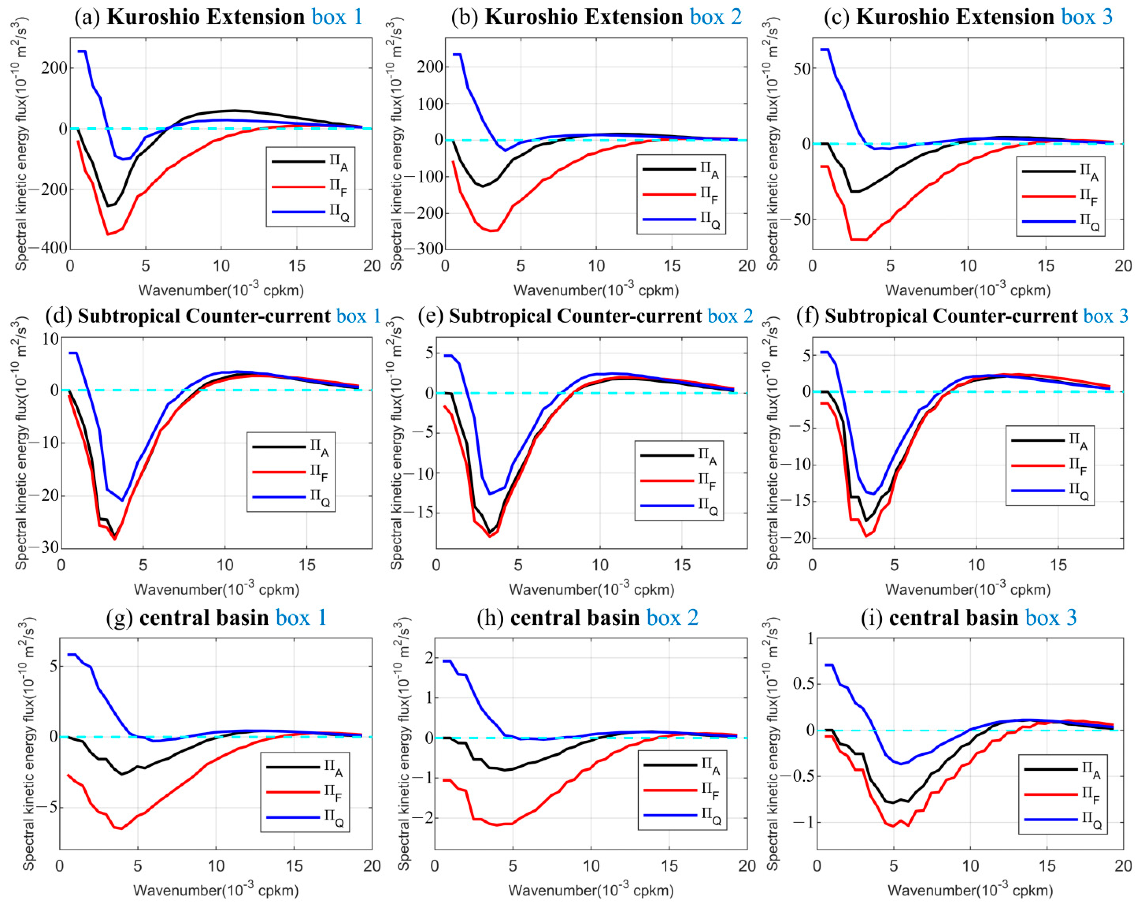
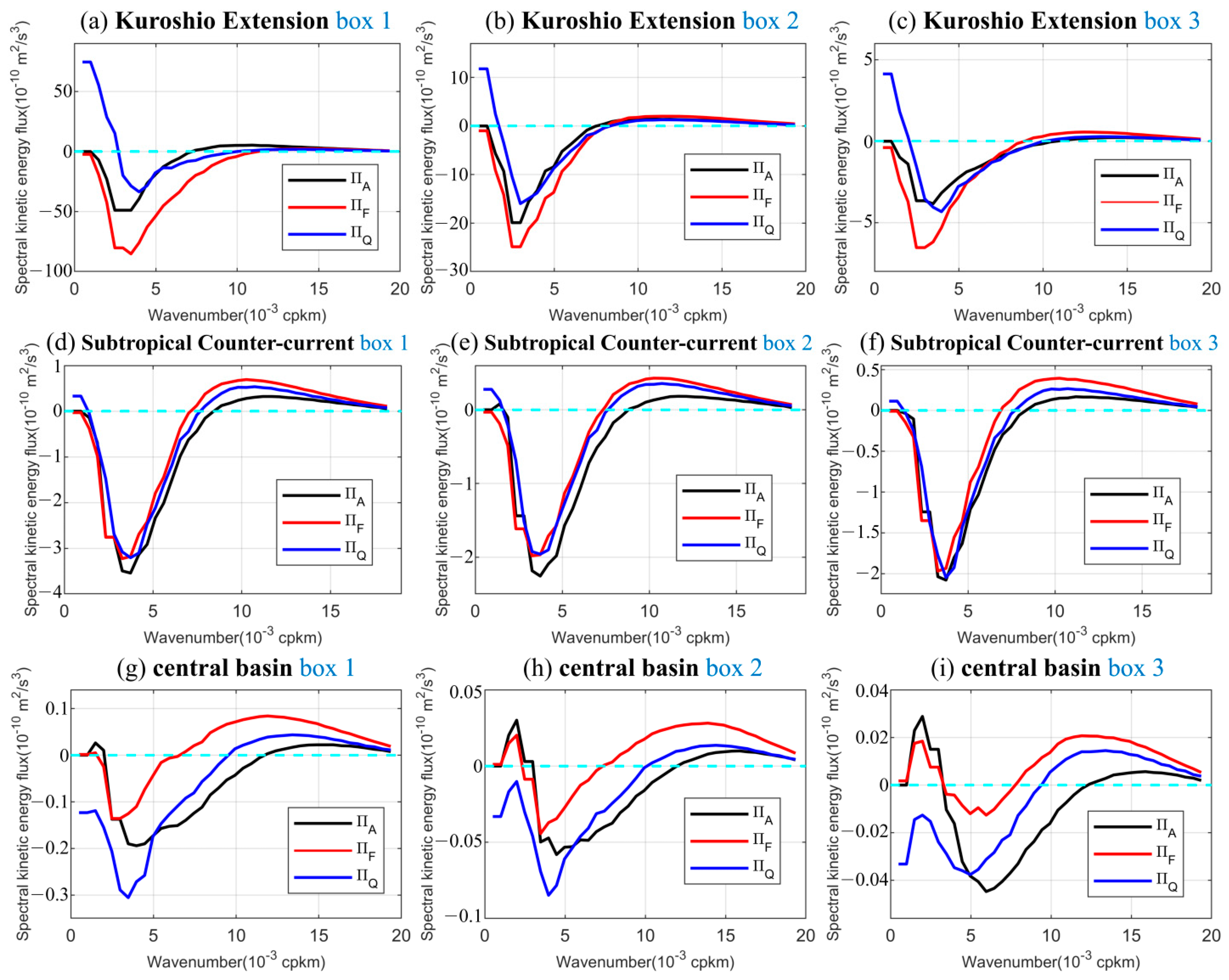
3.2. Diagnostic Results from Three Spectral Flux Definitions

This subsection compares the performance of these three definitions of spectral kinetic-energy flux in diagnosing kinetic-energy cascade. We focus on two metrics: the energy injection scale L_inj and the scale at which the upscale energy starts being arrested L_arrest-start (Figure 4). We follow Scott and Wang [12] and define the scale at which the inverse kinetic-energy cascade begins as the energy injection scale L_inj, that is, the scale corresponding to the zero point of the spectral flux with a positive slope. Following Wang et al. [18], we define the scale at which the spectral flux reaches minimum value as energy arrest-start scale L_arrest-start (Figure 4). These two scales have been widely studied and discussed. For example, Scott and Wang [12], Tulloch et al. [16] and Wang et al. [18] found L_inj to be in good agreement with the scale of maximum instability predicted by linear stability theory, indicating that baroclinic instability is the main source of upscale kinetic energy. The scale L_arrest-start is close to the observed eddy length scale and energy-containing scale (i.e., the scale of the most energetic eddies) [18,21]. In addition, the Rhines scale and the energy-containing scale coincide at latitudes where the inverse energy cascade occurs [46,47], which indicates L_arrest-start is also associated with the Rhines scale [48]. Our assessment of the sensitivity of L_inj and L_arrest-start to the choice of spectral flux definition will be useful for further unravelling the relation among these scales (e.g., L_inj, L_arrest-start, Rhines scale and the energy-containing scale) in the future.

We also consider a third metric: the amplitude of inverse cascade. Following Wang et al. [18] and Li et al. [19], we define this amplitude as the maximum negative value of spectral kinetic-energy flux. As such, it is a measure of the intensity of the inverse kinetic-energy cascade. Wang et al. [18] found this amplitude to have a spatial structure similar to that of the eddy kinetic energy. It is large in the energetic jet regions, such as the Antarctic Circumpolar Current and the Kuroshio Extension. It is also large in the Subtropical Countercurrents, whereas it is small in the central basin and gyre interiors.

Based on the spatial pattern of inverse cascade amplitude, we select three regions in the North Pacific to evaluate the performance of Π_Q, Π_F and Π_A: the Kuroshio Extension (KE) with a large amplitude, the Subtropical Countercurrent (STCC) with a middling amplitude, and the central basin with a small amplitude. For each region, we consider three subregions, labeled box 1, 2, and 3 in Figure 2.

Using each definition, we estimate the spectral energy fluxes in these nine subregions. The spectral energy fluxes in Figure 5 are estimated using the original velocity data. In the nine subregions, results from these three definitions share in the following two aspects.

One, all three have their largest amplitude in the Kuroshio Extension, followed by that for the Subtropical Countercurrents, and their smallest in the central basin of the North Pacific. The amplitude varies by more than two orders of magnitude. Thus, the inverse cascade amplitude is generally large in the regions with large eddy kinetic energy. These features agree with that in Wang et al. [18], which used definition I.

Two, all three definitions capture the inverse and forward kinetic-energy cascades in the North Pacific. At scales larger than L_inj, kinetic energy transfers to a larger scale, i.e., an inverse kinetic-cascade occurs. At scales smaller than L_inj, a forward kinetic-energy cascade occurs. This phenomenon is consistent with previous studies [12,18,19,21,22,23,49], which is called split cascades in Alexakis and Biferale [50]. The inverse kinetic-energy cascade at a large scale is a well-known phenomenon predicted by geostrophic turbulence theory [6]. Baroclinic instability is considered to be the source of upscale kinetic energy [18,51]. A forward cascade at small scales provides a route for direct dissipation of kinetic energy [23,24]. Some literature indicates that the occurrence of a forward cascade may be related to ageostrophic dynamics [22,23,24]. However, detailed mechanisms are to be explored.

Now we compare results based on the three definitions of spectral kinetic-energy fluxes. The energy injection scale L_inj diagnosed by the Π_Q definition is close to but slightly greater than that from the Π_A definition in most regions (Figure 5 and Figure 6). In the Kuroshio Extension and the central basin regions, L_inj from the Π_F definition is significantly smaller than those from Π_Q and Π_A (Figure 6). Consistently, the wavenumber range with a forward kinetic-energy cascade is very narrow for the Π_F definition (Figure 5). In the Subtropical Countercurrent regions, however, L_inj from all three definitions only have small differences (Figure 5 and Figure 6). The reason is that the energy transport in this region is relatively weak, and the ratio of the spatial transport of kinetic energy to cross-scale energy transfer is smaller (not shown), which reduces differences from definitions. In addition, as the wavenumber approaches zero, only the Π_A case approaches zero. The non-zero value of Π_Q at small wavenumbers occurs; because Π_Q includes the spatial transport of kinetic energy. With regard to Π_F, this case is affected by the background flow and these regions we considered do not satisfy the periodic boundary condition, which may contribute to the small, yet non-zero, value of Π_F at small wavenumbers.

We now repeat the analysis using preprocessed data. For these cases, we remove the spatial mean from surface velocity data and then multiply it with a Hamming window before applying the DFT. Compared to those using original velocity fields, the magnitudes of spectral fluxes from three definitions are all reduced by nearly an order of magnitude. Additionally, for the Π_A and Π_Q cases, in most regions we considered, the magnitudes of L_inj and L_arrset-start are slightly reduced due to preprocessing (Figure 5, Figure 6 and Figure 7). As to the Π_Q definition, the non-zero value of Π_Q at small wavenumbers exists regardless of preprocessing in the Kuroshio Extension and central basin regions. However, the deviation of Π_Q from zero at small wavenumbers gets reduced by preprocessing in the Subtropical Countercurrent regions. For the Π_F case, data preprocessing increases L_inj and causes the flux to vanish at small wavenumbers in all the nine regions we considered. This impact of data preprocessing on L_inj from Π_F is consistent with Aluie et al.’s [20] finding that data preprocessing shifts the flux curve to a larger scale.

These results indicate the following:

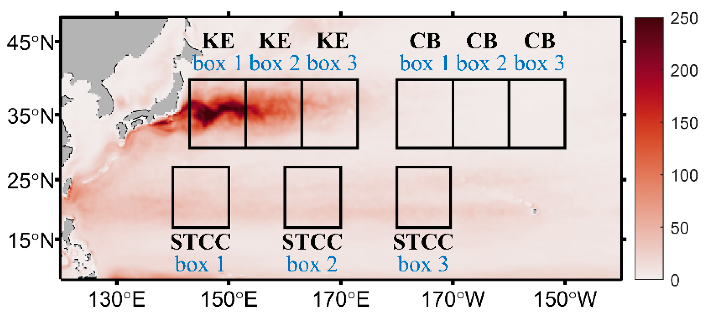
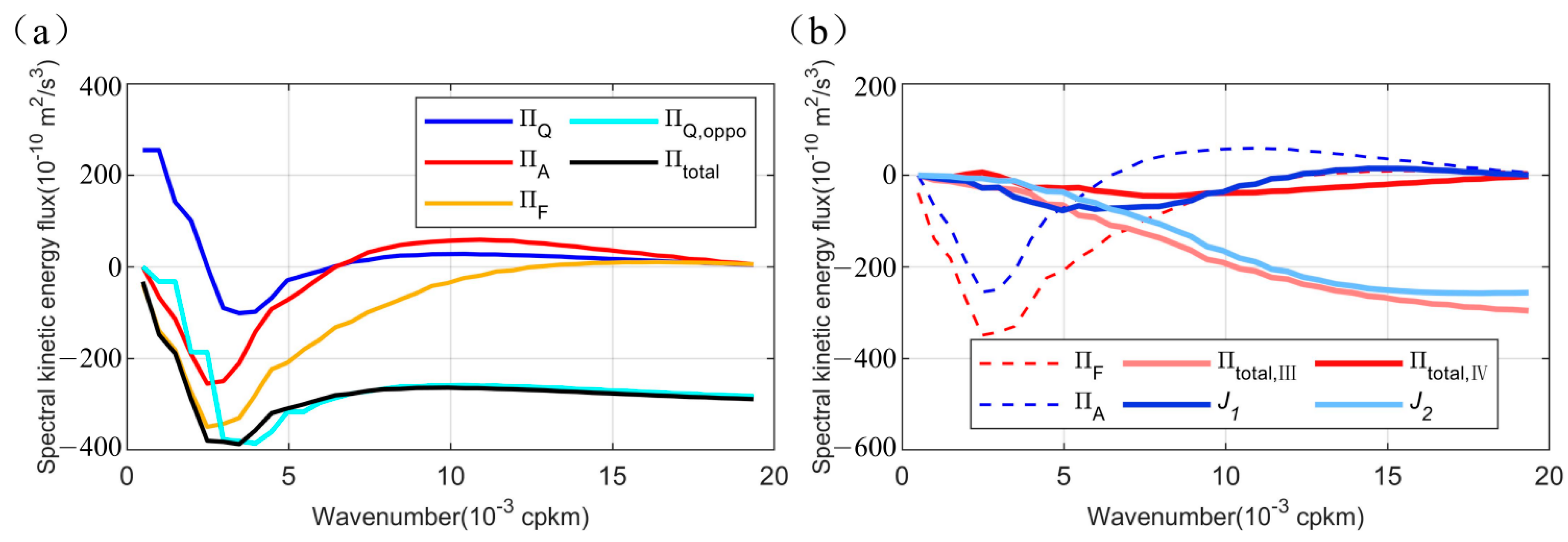
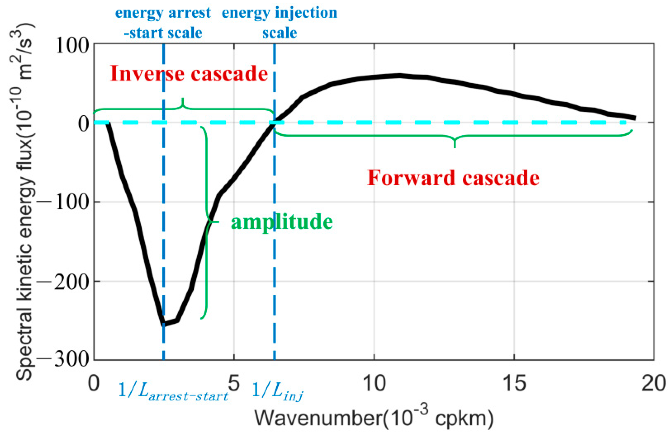
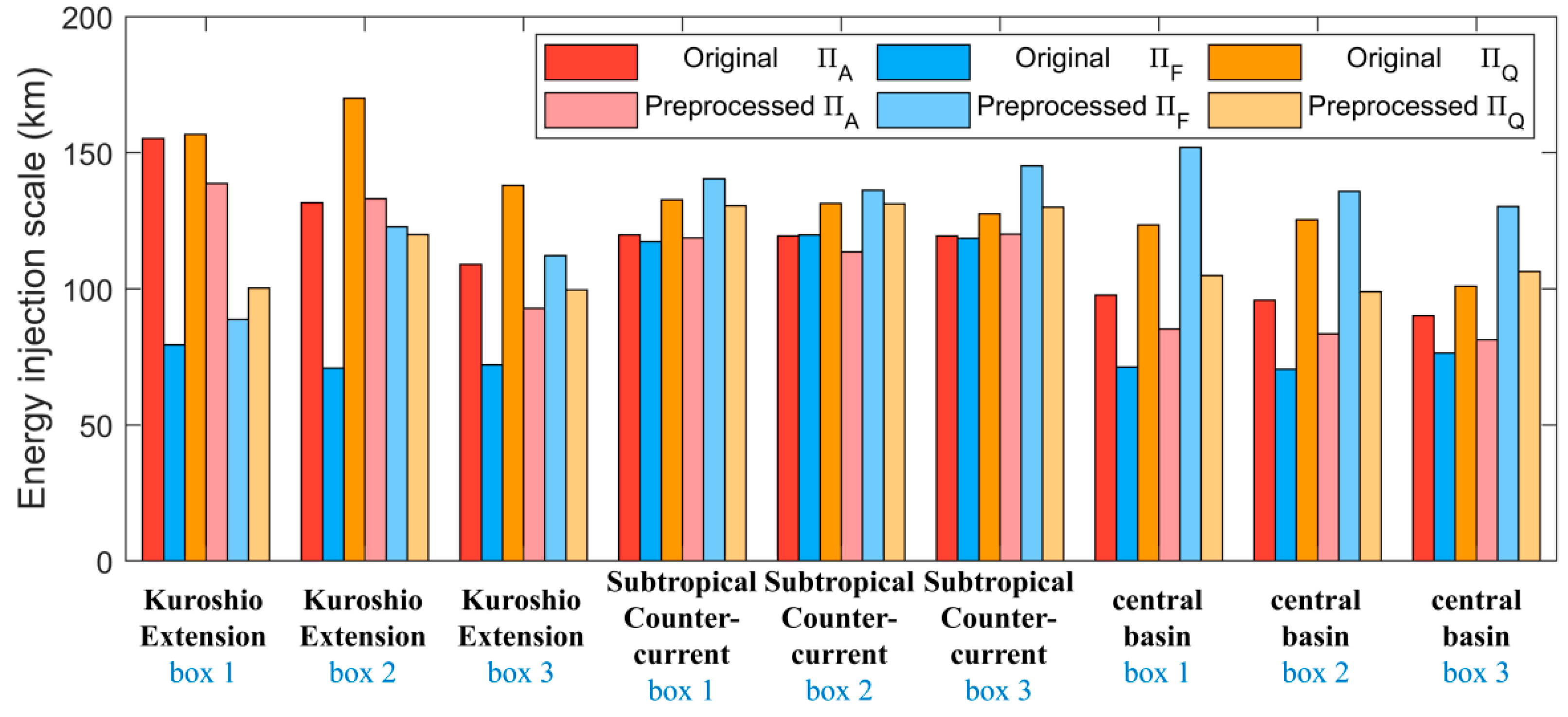
• For the Π_A case, the use of original velocity data generally leads to stable results. For spatial scale larger than L_inj, Π_A is negative, meaning the energy transfers to larger scale. The opposite happens below L_inj. The inverse cascade amplitude is generally larger in regions with a larger eddy kinetic energy. The value of L_inj is larger in the Kuroshio Extension and Subtropical Countercurrent regions than that in the quiescent central regions (Figure 6). Also, the spectral kinetic-energy flux approaches zero as wavenumber approaches zero or infinity. Finally, data preprocessing has little effect on the overall cascade features.
• For the Π_F case, the use of the preprocessed data leads to significantly different results from that from the original velocity data. The original is generally non-zero at wavenumbers near zero, whereas the preprocessed approaches zero as wavenumbers approach zero. The energy injection scale inferred from Π_F differs significantly from those from Π_Q and Π_A, particularly in the Kuroshio Extension and central basin regions. Data preprocessing reduces the difference of L_inj between the Π_A and Π_F definitions in the Kuroshio Extension regions, indicating that data preprocessing can weaken the influence of inhomogeneous flow on energy flux estimates.
• For the Π_Q case, the value of L_inj is comparable to that from the Π_A definition. However, the spectral energy fluxes from the Π_Q definition are significantly different from Π_F and Π_A at small wavenumbers. This difference arises because Π_Q includes spatial energy transport. Data preprocessing reduces the difference in spectral energy fluxes between the Π_Q definition and the other two definitions (Figure 5 and Figure 7).

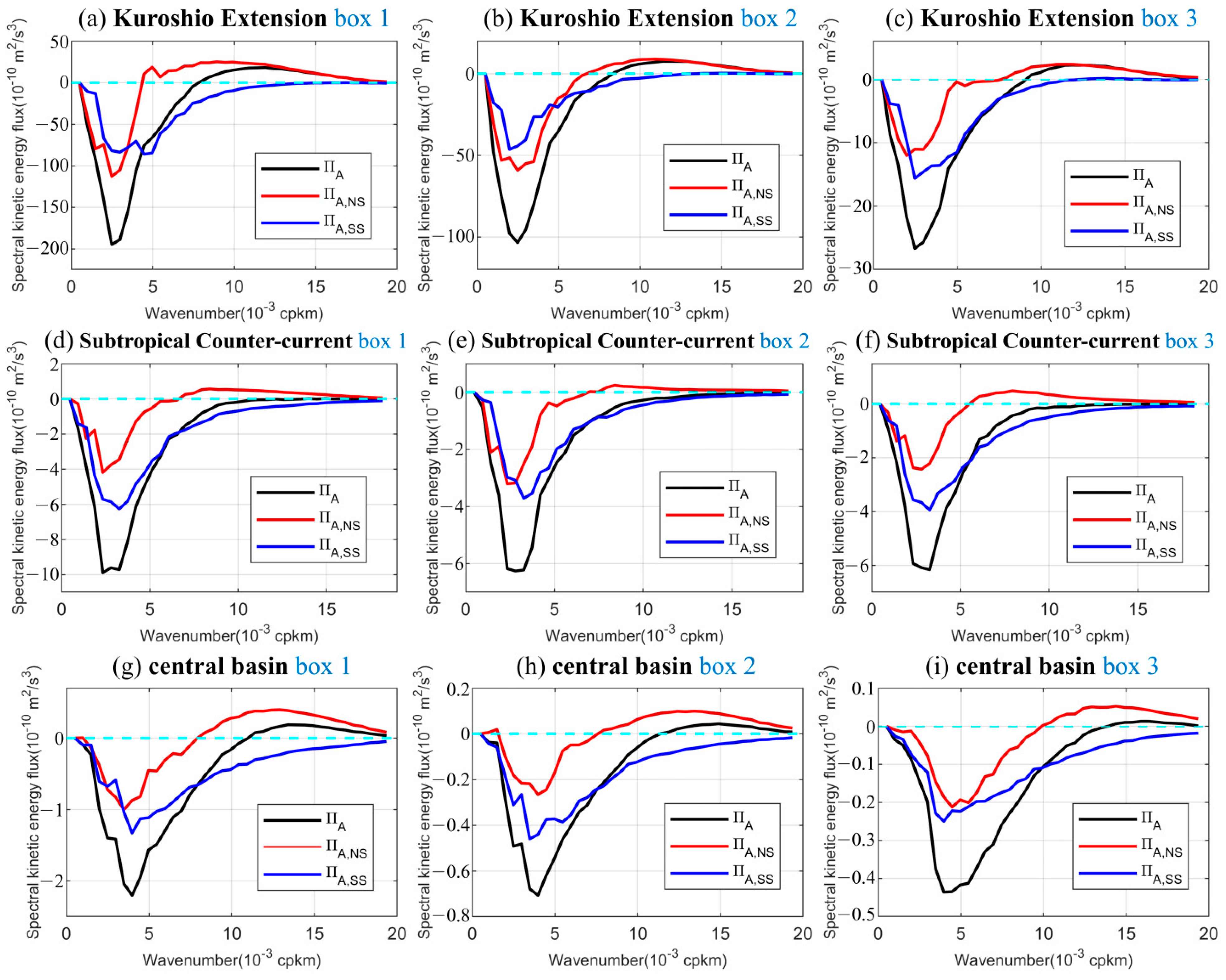
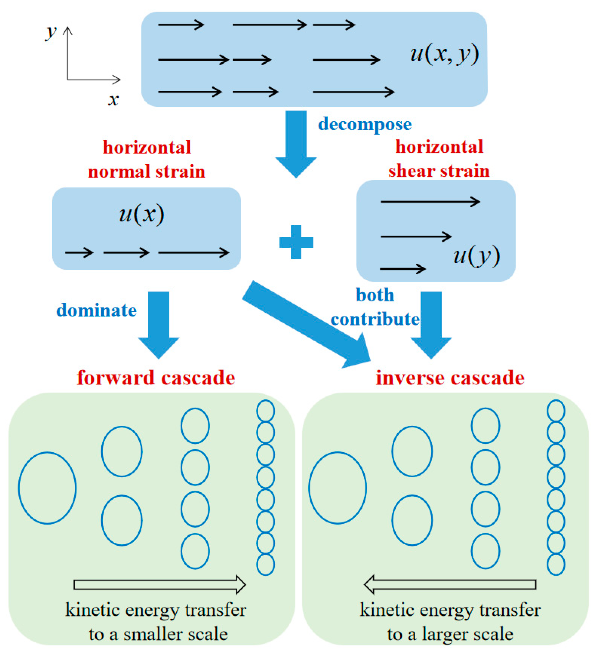
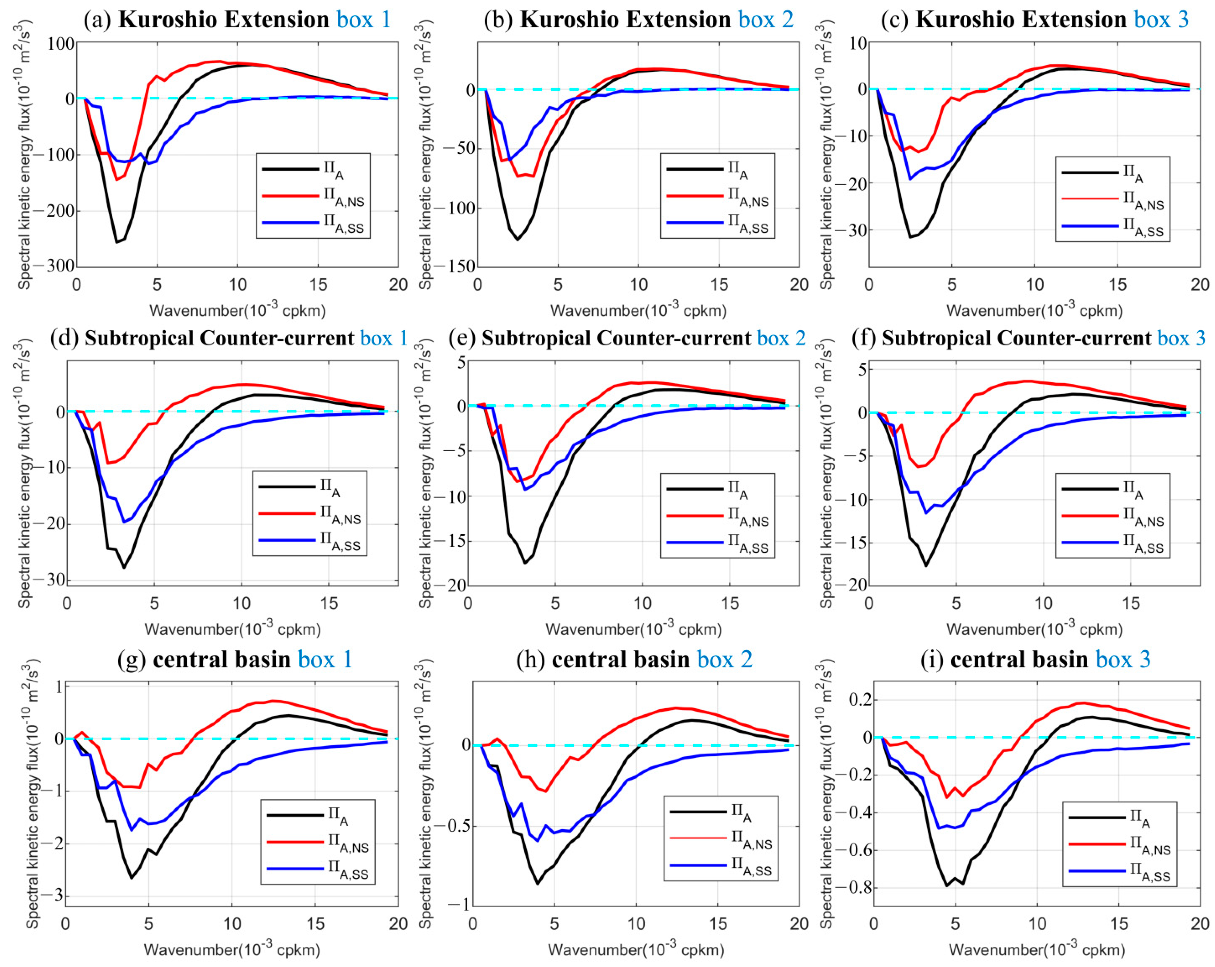
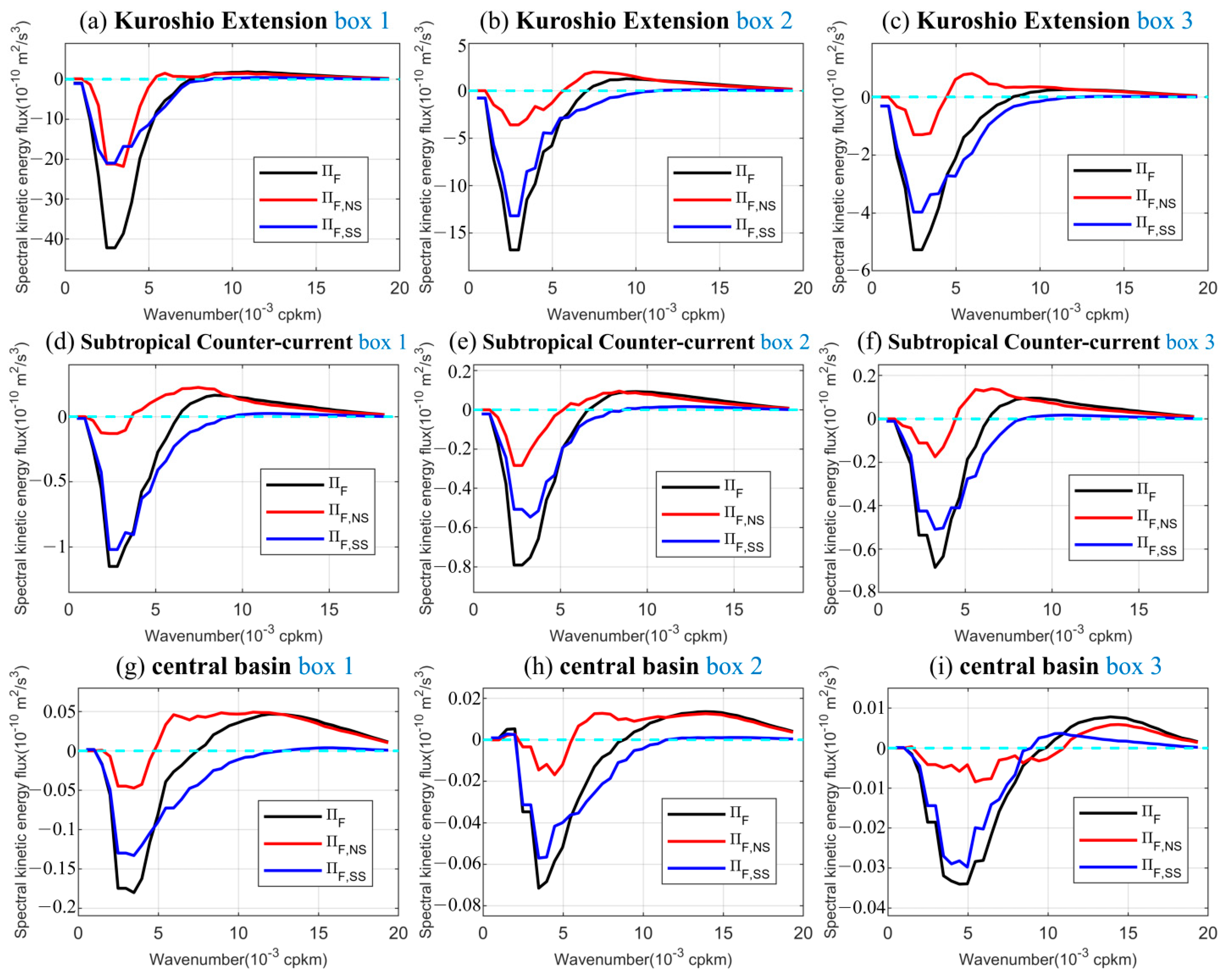
3.3. The Normal-Strain and Shear-Strain Decomposition of Spectral Kinetic-Energy Flux

The spectral kinetic-energy flux can be decomposed into two components: one component related to the horizontal normal strain ($\partial u/\partial x$ and $\partial v/\partial y$) and the other related to horizontal shear strain of the flow ($\partial u/\partial y$ and $\partial v/\partial x$). Although a similar decomposition of eddy-mean flow interaction has been shown to be useful in unraveling dynamics of submesoscale processes and tropical instability waves [27,28,29], it has apparently not been applied to energy cascade studies, despite the eddy-mean kinetic-energy exchange being a special form of kinetic-energy cascade. Here we estimate the contributions of horizontal normal and shear strains to kinetic-energy cascades in the North Pacific regions analyzed above.

For the estimates, we use the Π_A definition due to its results being generally stable in the regions we considered and the diagnosis not requiring data preprocessing. The normal-strain component of Π_A (Π_A,NS) and the shear-strain component (Π_A,SS) are, respectively,

$${\prod }_{\mathrm{A},NS}=〈[{(uu)}_K^{<}-u_K^{<}{u}_K^{<}]\frac{\partial u_K^{<}}{\partial x}+[{(vv)}_K^{<}-v_K^{<}{v}_K^{<}]\frac{\partial v_K^{<}}{\partial y}〉,$$

(24)

$${\prod }_{\mathrm{A},SS}=〈[{(uv)}_K^{<}-u_K^{<}{v}_K^{<}]\frac{\partial u_K^{<}}{\partial y}+[{(uv)}_K^{<}-u_K^{<}{v}_K^{<}]\frac{\partial v_K^{<}}{\partial x}〉.$$

(25)

We use the ECCO2 state estimate to diagnose these two terms from Equations (24) and (25) (Π_A,NS and Π_A,SS) in the selected regions in the North Pacific Ocean. Consistent with Aluie et al. [20], here we use the original velocity instead of preprocessed data for the analysis. We focus on the upper 500 m, where eddy kinetic energy is large and energy cascade is strong. Figure 8 and Figure 9 show the results at depths of 5 m and 100 m. The results at other depth levels in the upper 500 m are similar (not shown).

The results based on the Π_A definition show that inverse kinetic-energy cascade at large scales and forward cascade at small scales are prevalent phenomena in the upper 500 m in the selected subregions of the North Pacific. In one case, at the depth of 100 m in the North Pacific Subtropical Countercurrent, there is little forward cascade at any spatial scale (Figure 9d–f), which may be associated with the eastward countercurrent near this depth range in the region. A depth dependence of kinetic-energy cascade was also discussed in Wang et al. [18], where they found that the inverse kinetic-energy cascade exists at all depths in the global ocean. Additionally, Ajayi et al. [21] found that in the North Atlantic Ocean, an inverse cascade occurs at all depths at a large scale, whereas a forward cascade at a small scale occurs only near the surface.

The shear-strain component of the spectral flux, Π_A,SS, is always negative at all the available wavenumbers in the upper ocean in these selected regions, whereas the normal-strain component Π_A,NS is negative at large scales and positive at small scales. In other words, both the normal-strain and shear-strain components of the spectral kinetic flux from the Π_A definition contribute noticeably to the inverse kinetic-energy cascades at large scales. However, only the normal-strain component contributes to the forward cascade, and this occurs at small scales. Physically, the horizontal normal strain of the flow is related to the fluid-line deformation, and the shear strain is related to the fluid rotation and horizontal shear. Therefore, the above results indicate that the components related to rotation and flow shear in the ocean motion contribute to inverse kinetic-energy cascade as expected by geostrophic turbulence theory. Conversely, the components related to the fluid line deformation contribute to both forward kinetic-energy cascade at small scales and inverse cascade at large scales.

As an inverse cascade generally occurs at relatively large scales, where motions are nearly in geostrophic balance, we infer that forward cascade at small scales is closely related to ageostrophic flow and dynamics. This inference is consistent with the findings of several previous studies [22,24]. Our normal–shear strain decomposition of spectral kinetic-energy fluxes indicates that the contribution of ageostrophic motion to the forward kinetic-energy cascade is realized through Π_A,NS, i.e.,the normal-strain component of the spectral flux. The flow field with normal strain may induce strong fronts through frontogenesis, and these fronts further lead to instabilities that produce small-scale ageostrophic motions [52,53]. During this process, energy is transferred from large to small scales.

An analogous decomposition of spectral kinetic-energy flux has been explored previously [22,23,24,49]. These studies decomposed the velocity into a rotational part and a divergent part, and found that the rotational part leads to an inverse cascade, the divergent part instead leads to a forward cascade. Given that shear strain is related to flow rotation, and normal strain is related to flow divergence, our decomposition findings appear consistent with these studies.

Although the shear-strain component of the spectral flux, Π_A,SS, is negative at all scales and the normal-strain component Π_A,NS is negative only at large scales, the scales at which both Π_A,SS and Π_A,NS reach their maximum negative values are near L_arrest-start. Being near the energy arrest-start scale inferred from Π_A indicates that the upscale kinetic energy associated with the flow normal strain and shear strain may have the same sink. As L_arrest-start agrees well with eddy length scale and the scale of the most energetic eddies [18], the normal strain and shear strain of flow jointly influence these two scales associated with eddies through modulating energy cascade. In addition, the spatial scale at the zero crossing of Π_A,NS, which is larger than that of Π_A (i.e., L_inj), generally has larger magnitude in the Kuroshio Extension and Subtropical Countercurrent regions than that in the quiescent central regions.

Further, in the upstream of the Kuroshio Extension, the maximum negative value of the normal-strain component has larger magnitude than that of the shear strain component (Figure 8a,b). This result indicates that the contribution of normal strain to the inverse cascade is stronger than that of shear strain in the upstream Kuroshio Extension. However, in other regions, the maximum negative value of the shear-strain component has a larger magnitude than that of normal strain. We also find that in the upper ocean, L_arrest-start changes little with depth, though the inverse cascade amplitude decreases as depth increases (not shown). These results are consistent with those from Wang et al. [18] and Ajayi et al. [21]. In addition, we find that the magnitudes of both Π_A,SS and Π_A,NS decrease with depth. However, the scales at which Π_A,SS and Π_A,NS reach maximum negative values vary little with depth (not shown).

To see if these decomposition results are consistent with the use of another flux estimate, we apply the normal–shear strain decomposition to Π_F. As discussed in Section 3.1 and Section 3.2, the definitions of Π_F and Π_A are similar in their physical meanings and derivation methods. However, Π_F may be affected by inhomogeneous background flow, and the L_inj results inferred from the Π_F and Π_A definitions are significantly different in the Kuroshio Extension and central basin regions. So, we apply the data preprocessing to the Π_F case.

The normal-strain component of Π_F (Π_F,NS) and the shear-strain component (Π_F,SS) are, respectively,

$${\prod }_{\mathrm{F},NS}=〈u_K^{<}u\frac{\partial u_K^{>}}{\partial x}+v_K^{<}v\frac{\partial v_K^{>}}{\partial y}〉,$$

(26)

$${\prod }_{\mathrm{F},SS}=〈u_K^{<}v\frac{\partial u_K^{>}}{\partial y}+v_K^{<}u\frac{\partial v_K^{>}}{\partial x}〉.$$

(27)

The representative results of Π_F,NS and Π_F,SS at 100 m depth are shown in Figure 10. The key findings about this decomposition based on the previous definition (Π_A) also apply here. We discuss four such findings. One, for the upper ocean, both the normal- and shear-strain components of the spectral flux from the Π_F definition contribute to the inverse cascade at large scales, and only the normal-strain components contribute to the forward cascade at small scales. Yet, the exception occurs at the surface in the central basin of the North Pacific such as CB box 2 and CB box 3, where positive Π_F,SS occurs at a small scale. This exception may be due to the influence of the background flow structure on the Π_F estimates and the spurious flow characteristics introduced by data preprocessing. Two, the scales at which Π_F,SS and Π_F,NS reach their maximum negative values are close to the L_arrest-start inferred from total spectral flux Π_F in most regions. Three, in the upstream of the Kuroshio Extension, the maximum negative value of the normal-strain component is close to that of the shear-strain component, indicating that the upscale kinetic energy associated with the normal strain is roughly equal to that from the shear strain (Figure 10a). In other regions, the maximum absolute value of the shear-strain component exceeds that of the normal-strain component. This means that in these regions, the shear strain component contributes more to inverse cascade than the normal-strain component. Finally, the magnitudes of Π_F,SS and Π_F,NS decrease with depth. Yet, the spatial scales at which Π_F,SS and Π_F,NS reach maximum negative values change little with depth (not shown).

The Π_Q definition of spectral kinetic-energy flux includes energy transport in space (Section 2). This part of Π_Q can also be decomposed into normal- and shear-strain components, which leads to the normal–shear strain decomposition of Π_Q containing information about both the energy cascade and spatial energy transport. Therefore, we consider the decomposition method based on Π_Q inappropriate to assess the separate contributions of normal strain and shear strain to the energy cascade (results unshown).

4. Conclusions

The spectral kinetic-energy flux is a useful metric to quantify the transfer of kinetic energy across length scales. In this paper, we compared results from three diagnosis methods about this flux. All three methods originate from the advection term in the momentum equation. Both the Π_F and Π_A definitions exclude a transport term and only retain the part related to the redistribution of kinetic energy across different scales. However, this excluded transport term differs between the definitions. As a result, Π_A satisfies Galilean invariance, but Π_F does not and thus is affected by inhomogeneous background flow. The third definition is Π_Q, which includes an energy spatial transport term.

Using the ECCO2 state estimate, we analyzed the spectral kinetic-energy flux from the three definitions in several regions of the North Pacific. In general, all three definitions showed an inverse kinetic-energy cascade at low wavenumbers and a forward cascade at high wavenumbers. Specifically, at the spatial scale larger than L_inj, kinetic energy transferred to a larger scale. At scales smaller than L_inj, however, kinetic energy transferred to a smaller scale. In addition, for all definitions, the inverse cascade amplitude is generally larger in region with larger eddy kinetic energy.

The spectral energy fluxes from these definitions also showed differences. For example, the Π_A definition generally produced stable results with no need for data preprocessing. The Π_F definition, however, was affected by the background flow. In some regions, such as the Kuroshio Extension and the central basin, the value of L_inj from Π_F differed significantly from those of Π_Q and Π_A. However, the use of data preprocessing (removing spatial mean and multiplying by a Hamming window) reduced these differences. Although the energy-injection scale inferred from the Π_Q definition was reasonable, at small wavenumbers, the spectral energy flux from the Π_Q definition differed significantly from those of Π_F and Π_A. We argued that this difference arose from Π_Q containing the energy spatial transport term.

In the second part of the paper, we decomposed the spectral energy fluxes into the horizontal normal-strain and shear-strain components. We used the same state estimate to assess this decomposition in the same regions in the upper ocean of the North Pacific. For the Π_A definition, both the normal- and shear-strain components contribute noticeably to the inverse kinetic-energy cascades at low wavenumbers. However, only the normal-strain component contributed to the forward kinetic-energy cascade at high wavenumbers (Figure 11). Running the same decomposition using the Π_F definition generally gave the same results as those using Π_A. However, the Π_Q definition is not suitable for assessing this decomposition of spectral energy fluxes. This is because the Π_Q definition contains an energy transport term that can also be decomposed into normal- and shear-strain components. This term essentially represents the spatial transport of energy, not energy transfer across different spatial scales.

In general, the findings here should help the community to choose the appropriate method to examine energy cascade in future studies. Additionally, the use of the normal-strain and shear-strain decomposition of spectral energy fluxes should help shed light on the underlying mechanisms of forward and inverse cascades. However, this study has the following limitations: (1) The discussion is only focused on the North Pacific; (2) the spectral truncation method is used for eliminating the high wavenumber Fourier components, and other filtering methods are not discussed; (3) the numerical model analyzed here is eddy-permitting and does not include tidal forcing; however, Ajayi et al. [21] found high-frequency and non-geostrophic motions play a key role in the forward cascade.

Possible future work includes (1) assessing the effect of spatial filter methods on energy cascade features; (2) extending the analysis to different regions or time periods; (3) revisiting this problem using observations and submesoscale-permitting models; (4) estimating the potential- and total-energy flux (e.g., Schlösser and Eden [15]), helicity flux (e.g., Alexakis [54]) and enstrophy flux (e.g., Khatri et al. [55]), besides the kinetic-energy flux analyzed here; (5) further exploring the mechanism of the forward kinetic-energy cascade at small scales, for example, discussing the role of small-scale tidal motions on forward cascade (e.g., Arbic [56]), or the influence of stratification and rotation on forward cascade (e.g., Marino et al. [57]), and; (6) applying machine learning approach and these spectral flux definitions to predict spectral fluxes, analogous to the prediction of eddy heat fluxes by George et al. [58].

References

1. Qiu, B.; Scott, R.B.; Chen, S.M. Length scales of eddy generation and nonlinear evolution of the seasonally modulated South Pacific Subtropical Countercurrent. J. Phys. Oceanogr. 2008, 38, 1515–1528. [Google Scholar] [CrossRef]
2. Zhang, Z.G.; Zhang, Y.; Wang, W.; Huang, R.X. Universal structure of mesoscale eddies in the ocean. Geophys. Res. Lett. 2013, 40, 3677–3681. [Google Scholar] [CrossRef]
3. Gill, A.E. Atmosphere–Ocean Dynamics; Academic Press: New York, NY, USA, 1982; p. 662. [Google Scholar]
4. Pedlosky, J. Geophysical Fluid Dynamics; Springer: New York, NY, USA, 1987; p. 710. [Google Scholar]
5. Taylor, G. Observations and Speculations on the Nature of Turbulent Motion; Cambridge University Press: New York, NY, USA, 1917; p. 69. [Google Scholar]
6. Charney, J.G. Geostrophic Turbulence. J. Atmos. Sci. 1971, 28, 1087–1095. [Google Scholar] [CrossRef]
7. Salmon, R. Two-layer quasi-geostrophic turbulence in a simple special case. Geophys. Astrophys. Fluid Dyn. 1978, 10, 25–52. [Google Scholar] [CrossRef]
8. Salmon, R. Baroclinic instability and geostrophic turbulence. Geophys. Astrophys. Fluid Dyn. 1980, 15, 167–211. [Google Scholar] [CrossRef]
9. Salmon, R.L. Lecture on Geophysical Fluid Dynamics; Oxford University Press: New York, NY, USA, 1998; p. 378. [Google Scholar]
10. Fu, L.L.; Flierl, G.R. Nonlinear energy and enstrophy transfers in a realistically stratified ocean. Dyn. Atmos. Oceans 1980, 4, 219–246. [Google Scholar] [CrossRef]
11. Frisch, U. Turbulence: The Legacy of A. N. Kolmogorov; Cambridge University Press: New York, NY, USA, 1995; p. 296. [Google Scholar]
12. Scott, R.B.; Wang, F.M. Direct evidence of an oceanic inverse kinetic energy cascade from satellite altimetry. J. Phys. Oceanogr. 2005, 35, 1650–1666. [Google Scholar] [CrossRef]
13. Wunsch, C. The vertical partition of oceanic horizontal kinetic energy. J. Phys. Oceanogr. 1997, 27, 1770–1794. [Google Scholar] [CrossRef]
14. Scott, R.B.; Arbic, B.K. Spectral energy fluxes in geostrophic turbulence: Implications for ocean energetics. J. Phys. Oceanogr. 2007, 37, 673–688. [Google Scholar] [CrossRef]
15. Schlösser, F.; Eden, C. Diagnosing the energy cascade in a model of the North Atlantic. Geophys. Res. Lett. 2007, 34, L02604. [Google Scholar] [CrossRef]
16. Tulloch, R.; Marshall, J.; Hill, C.; Smith, K.S. Scales, Growth Rates, and Spectral Fluxes of Baroclinic Instability in the Ocean. J. Phys. Oceanogr. 2011, 41, 1057–1076. [Google Scholar] [CrossRef]
17. Arbic, B.K.; Polzin, K.L.; Scott, R.B.; Richman, J.G.; Shriver, J.F. On Eddy Viscosity, Energy Cascades, and the Horizontal Resolution of Gridded Satellite Altimeter Products. J. Phys. Oceanogr. 2013, 43, 283–300. [Google Scholar] [CrossRef]
18. Wang, S.; Liu, Z.; Pang, C. Geographical distribution and anisotropy of the inverse kinetic energy cascade, and its role in the eddy equilibrium processes. J. Geophys. Res. Oceans 2015, 120, 4891–4906. [Google Scholar] [CrossRef]
19. Li, H.J.; Xu, Y.S. Barotropic and Baroclinic Inverse Kinetic Energy Cascade in the Antarctic Circumpolar Current. J. Phys. Oceanogr. 2021, 51, 809–824. [Google Scholar] [CrossRef]
20. Aluie, H.; Hecht, M.; Vallis, G.K. Mapping the Energy Cascade in the North Atlantic Ocean: The Coarse-Graining Approach. J. Phys. Oceanogr. 2018, 48, 225–244. [Google Scholar] [CrossRef]
21. Ajayi, A.; Le Sommer, J.; Chassignet, E.P.; Molines, J.M.; Xu, X.B.A.; Albert, A.; Dewar, W. Diagnosing Cross-Scale Kinetic Energy Exchanges From Two Submesoscale Permitting Ocean Models. J. Adv. Model. Earth Syst. 2021, 13, e2019MS001923. [Google Scholar] [CrossRef]
22. Capet, X.; McWilliams, J.C.; Molemaker, M.J.; Shchepetkin, A.F. Mesoscale to submesoscale transition in the California current system. Part III: Energy balance and flux. J. Phys. Oceanogr. 2008, 38, 2256–2269. [Google Scholar] [CrossRef]
23. Molemaker, M.J.; McWilliams, J.C.; Capet, X. Balanced and unbalanced routes to dissipation in an equilibrated Eady flow. J. Fluid Mech. 2010, 654, 35–63. [Google Scholar] [CrossRef]
24. Brüggemann, N.; Eden, C. Routes to Dissipation under Different Dynamical Conditions. J. Phys. Oceanogr. 2015, 45, 2149–2168. [Google Scholar] [CrossRef]
25. Weisberg, R.H.; Weingartner, T.J. Instability waves in the Equatorial Atlantic Ocean. J. Phys. Oceanogr. 1988, 18, 1641–1657. [Google Scholar] [CrossRef]
26. Luther, D.S.; Johnson, E.S. Eddy Energetics in the Upper Equatorial Pacific during the Hawaii-to-Tahiti Shuttle Experiment. J. Phys. Oceanogr. 1990, 20, 913–944. [Google Scholar] [CrossRef]
27. Qiao, L.; Weisberg, R.H. Tropical instability wave energetics: Observations from the tropical instability wave experiment. J. Phys. Oceanogr. 1998, 28, 345–360. [Google Scholar] [CrossRef]
28. Masina, S.; Philander, S.G.H.; Bush, A.B.G. An analysis of tropical instability waves in a numerical model of the Pacific Ocean: 2. Generation and energetics of the waves. J. Geophys. Res. Oceans 1999, 104, 29637–29661. [Google Scholar] [CrossRef]
29. Holmes, R.M.; Thomas, L.N. Modulation of Tropical Instability Wave Intensity by Equatorial Kelvin Waves. J. Phys. Oceanogr. 2016, 46, 2623–2643. [Google Scholar] [CrossRef]
30. Wang, S.; Jing, Z.; Liu, H.; Wu, L. Spatial and Seasonal Variations of Submesoscale Eddies in the Eastern Tropical Pacific Ocean. J. Phys. Oceanogr. 2018, 48, 101–116. [Google Scholar] [CrossRef]
31. Wang, M.; Du, Y.; Qui, B.; Xie, S.-P.; Feng, M. Dynamics on Seasonal Variability of EKE Associated with TIWs in the Eastern Equatorial Pacific Ocean. J. Phys. Oceanogr. 2019, 49, 1503–1519. [Google Scholar] [CrossRef]
32. Cao, H.J.; Fox-Kemper, B.; Jing, Z.Y. Submesoscale Eddies in the Upper Ocean of the Kuroshio Extension from High-Resolution Simulation: Energy Budget. J. Phys. Oceanogr. 2021, 51, 2181–2201. [Google Scholar] [CrossRef]
33. Wunsch, C.; Heimbach, P.; Ponte, R.M.; Fukumori, I. The global general circulation of the ocean estimated by the ECCO-Consortium. Oceanography 2009, 22, 88–103. [Google Scholar] [CrossRef]
34. Chen, R.; Flierl, G.R.; Wunsch, C. A Description of Local and Nonlocal Eddy-Mean Flow Interaction in a Global Eddy-Permitting State Estimate. J. Phys. Oceanogr. 2014, 44, 2336–2352. [Google Scholar] [CrossRef]
35. Chen, R.; Thompson, A.F.; Flierl, G.R. Time-Dependent Eddy-Mean Energy Diagrams and Their Application to the Ocean. J. Phys. Oceanogr. 2016, 46, 2827–2850. [Google Scholar] [CrossRef]
36. Qiu, B.; Chen, S.M.; Schneider, N. Dynamical Links between the Decadal Variability of the Oyashio and Kuroshio Extensions. J. Clim. 2017, 30, 9591–9605. [Google Scholar] [CrossRef]
37. Yang, Q.; Zhao, W.; Liang, X.; Dong, J.; Tian, J. Elevated Mixing in the Periphery of Mesoscale Eddies in the South China Sea. J. Phys. Oceanogr. 2017, 47, 895–907. [Google Scholar] [CrossRef]
38. Dong, J.; Fox-Kemper, B.; Zhang, H.; Dong, C. The Seasonality of Submesoscale Energy Production, Content, and Cascade. Geophys. Res. Lett. 2020, 47, e2020GL087388. [Google Scholar] [CrossRef]
39. Domaradzki, J.A.; Rogallo, R.S. Local energy transfer and nonlocal interactions in homogeneous, isotropic turbulence. Phys. Fluids A 1990, 2, 413–426. [Google Scholar] [CrossRef]
40. Maltrud, M.E.; Vallis, G.K. Energy and enstrophy transfer in numerical simulations of two-dimensional turbulence. Phys. Fluids A 1993, 5, 1760–1775. [Google Scholar] [CrossRef]
41. Chen, R. Energy Pathways and Structures of Oceanic Eddies from the ECCO2 State Estimate and Simplified Models. Ph.D. Thesis, Massachusetts Institute of Technology, Cambridge, MA, USA, 2013. [Google Scholar]
42. Marshall, J.; Adcroft, A.; Hill, C.; Perelman, L.; Heisey, C. A finite-volume, incompressible Navier Stokes model for studies of the ocean on parallel computers. J. Geophys. Res. Ocean. 1997, 102, 5753–5766. [Google Scholar] [CrossRef]
43. Marshall, J.; Hill, C.; Perelman, L.; Ad Croft, A. Hydrostatic, quasi-hydrostatic, and nonhydrostatic ocean modeling. J. Geophys. Res. Ocean. 1997, 102, 5733–5752. [Google Scholar] [CrossRef]
44. Large, W.G.; Mcwilliams, J.C.; Doney, S.C. Oceanic vertical mixing: A review and a model with a nonlocal boundary layer parameterization. Rev. Geophys. 1994, 32, 363–403. [Google Scholar] [CrossRef]
45. Sasaki, H.; Klein, P. SSH wavenumber spectra in the North Pacific from a high-resolution realistic simulation. J. Phys. Oceanogr. 2012, 42, 1233–1241. [Google Scholar] [CrossRef]
46. Chemke, R.; Dror, T.; Kaspi, Y. Barotropic kinetic energy and enstrophy transfers in the atmosphere. Geophys. Res. Lett. 2016, 43, 7725–7734. [Google Scholar] [CrossRef]
47. Chemke, R.; Kaspi, Y. The latitudinal dependence of the oceanic barotropic eddy kinetic energy and macroturbulence energy transport. Geophys. Res. Lett. 2016, 43, 2723–2731. [Google Scholar] [CrossRef]
48. Rhines, P.B. Waves and turbulence on a beta-plane. J. Fluid Mech. 1975, 69, 417–443. [Google Scholar] [CrossRef]
49. Klein, P.; Hua, B.L.; Lapeyre, G.; Capet, X.; Le Gentil, S.; Sasaki, H. Upper ocean turbulence from high-resolution 3D simulations. J. Phys. Oceanogr. 2008, 38, 1748–1763. [Google Scholar] [CrossRef]
50. Alexakis, A.; Biferale, L. Cascades and transitions in turbulent flows. Phys. Rep. 2018, 767, 1–101. [Google Scholar] [CrossRef]
51. Ferrari, R.; Wunsch, C. Ocean Circulation Kinetic Energy: Reservoirs, Sources, and Sinks. Annu. Rev. Fluid Mech. 2009, 41, 253–282. [Google Scholar] [CrossRef]
52. Cushman-Roisin, B.; Beckers, J. Introduction to Geophysical Fluid Dynamics; Academic Press: New York, NY, USA, 2009; p. 482. [Google Scholar]
53. McWilliams, J.C. Oceanic Frontogenesis. Annu. Rev. Mar. Sci. 2021, 13, 227–253. [Google Scholar] [CrossRef] [PubMed]
54. Alexakis, A. Helically decomposed turbulence. J. Fluid Mech. 2017, 812, 752–770. [Google Scholar] [CrossRef]
55. Khatri, H.; Sukhatme, J.; Kumar, A.; Verma, M.K. Surface ocean enstrophy, kinetic energy fluxes, and spectra from satellite altimetry. J. Geophys. Res. Oceans 2018, 123, 3875–3892. [Google Scholar] [CrossRef]
56. Arbic, B.K. Incorporating tides and internal gravity waves within global ocean general circulation models: A review. Prog. Oceanogr. 2022, 206, 102824. [Google Scholar] [CrossRef]
57. Marino, R.; Pouquet, A.; Rosenberg, D. Resolving the Paradox of Oceanic Large-Scale Balance and Small-Scale Mixing. Phys. Rev. Lett. 2015, 114, 114504. [Google Scholar] [CrossRef]
58. George, T.M.; Manucharyan, G.E.; Thompson, A.F. Deep learning to infer eddy heat fluxes from sea surface height patterns of mesoscale turbulence. Nat. Commun. 2021, 12, 800. [Google Scholar] [CrossRef] [PubMed]
Figure 1. Spectral kinetic-energy fluxes on rectangular domain centered on 22° N, 165° E with different sizes (30 × 30, 40 × 40, 60 × 60, 80 × 80, 80 × 40, 60 × 40 grid points). Only taking ΠA definition as an example, and the fluxes are based on the surface velocity of ECCO2 model without data preprocessing.
Jmse 10 01148 g001
Figure 2. Time mean surface eddy kinetic energy ( u u ¯ + v v ¯ ) / 2 (m2/s2) from the ECCO2 state estimate. u’ and v’ are zonal and meridional velocity anomalies defined as the deviation from the time-mean over the years 1992–2003. The KE boxes (10° × 10°) are located in the Kuroshio Extension, STCC in the North Pacific Subtropical Countercurrent, and CB in the central basin of the North Pacific.
Jmse 10 01148 g002
Figure 3. Spectral kinetic-energy fluxes. (a) Time-mean of ΠQ, ΠA, ΠF, ΠQ,oppo, and Πtotal [Equations (6), (22), (16), (7), and (15)]. (b) Time-mean of ΠA, ΠF, the transport of large-scale kinetic energy Πtotal,III, Πtotal,IV [Equation (15)], J1, J2 [Equation (23)]. All quantities are for the KE box 1 region from Figure 2. Analysis here is based on the surface velocity output from the ECCO2 model without data preprocessing.
Jmse 10 01148 g003
Figure 4. Energy injection scale and energy arrest-start scale. Positive and negative spectral flux indicate forward and inverse cascades, respectively. The energy injection scale Linj marks the crossing of inverse to forward cascade, the maximum negative flux marks the energy arrest-start scale Larrest-start. This maximum negative value is defined as the amplitude of inverse kinetic-energy cascade. Black curve just serves as an example (ΠA, from Figure 3a).
Jmse 10 01148 g004
Figure 5. Time-mean surface spectral kinetic-energy flux ΠA, ΠF, and ΠQ in the nine subregions marked in Figure 2. Each box has 40 × 40 grid points. Results here are estimated from the original velocity data without preprocessing.
Jmse 10 01148 g005
Figure 6. Energy injection scale Linj from ΠA, ΠF, and ΠQ in the nine subregions shown in Figure 2.
Jmse 10 01148 g006
Figure 7. Same as Figure 5 except based on the preprocessed velocity data.
Jmse 10 01148 g007
Figure 8. Time-mean of the total, normal-strain [ΠA,NS, Equation (24)], and shear-strain [ΠA,SS, Equation (25)] components to the spectral kinetic-energy flux ΠA at a depth of 5 m in the nine regions from Figure 2. The title of each panel indicates the name of each region. No preprocessing of velocity is applied in this diagnosis.
Jmse 10 01148 g008
Figure 9. Time-mean of the total, normal-strain [ΠA,NS, Equation (24)], and shear-strain [ΠA,SS, Equation (25)] components to the spectral kinetic-energy flux ΠA at a depth of 100 m in the nine regions from Figure 2. The title of each panel indicates the name of each region. No pre-processing of velocity is applied.
Jmse 10 01148 g009
Figure 10. Same as Figure 9 (i.e., at 100 m) except using ΠF with preprocessed velocity data.
Jmse 10 01148 g010
Figure 11. The role of horizontal normal strain and shear strain of flow in the kinetic-energy cascade in the upper ocean. We show here an arbitrary pure zonal flow u, decomposed into flows containing horizontal normal strain and shear strain. In the North Pacific regions we considered here, forward kinetic-energy cascade is dominated by the former, whereas the inverse cascade comes from both.
Jmse 10 01148 g011
Publisher’s Note: MDPI stays neutral with regard to jurisdictional claims in published maps and institutional affiliations.