Improved Robust High-Degree Cubature Kalman Filter Based on Novel Cubature Formula and Maximum Correntropy Criterion with Application to Surface Target Tracking

Abstract

Robust nonlinear filtering is an important method for tracking maneuvering targets in non-Gaussian noise environments. Although there are many robust filters for nonlinear systems, few of them have ideal performance for mixed Gaussian noise and non-Gaussian noise (such as scattering noise) in practical applications. Therefore, a novel cubature formula and maximum correntropy criterion (MCC)-based robust cubature Kalman filter is proposed. First, the fully symmetric cubature criterion and high-order divided difference are used to construct a new fifth-degree cubature formula using fewer symmetric cubature points. Then, a new cost function is obtained by combining the weighted least-squares method and the MCC loss criterion to deal with the abnormal values of non-Gaussian noise, which enhances the robustness; and statistical linearization methods are used to calculate the approximate result of the measurement process. Thus, the final fifth-degree divided difference–maximum correntropy cubature Kalman filter (DD-MCCKF) framework is constructed. A typical surface-maneuvering target-tracking simulation example is used to verify the tracking accuracy and robustness of the proposed filter. Experimental results indicate that the proposed filter has a higher tracking accuracy and better numerical stability than other common nonlinear filters in non-Gaussian noise environments with fewer cubature points used.

1. Introduction

Accurate and robust state estimation is important for the stable target tracking of conventional ships and surface unmanned ships. It is one of the main target-tracking processes for realizing sensor data fusion and anti-interference performance via a filtering algorithm. For linear Gaussian state space models, the Kalman filter (KF) is a powerful optimal estimation algorithm based on minimum mean square error. It is the most widely used adaptive filter because of its analytical optimality, algorithm stability, and simplicity. However, most commonly used target-tracking models are nonlinear, and this limits the role of the traditional KF, which only applies to linear models in practical applications.

Therefore, a nonlinear filtering algorithm in the Gaussian filter framework is required for target tracking. The extended Kalman filter (EKF) [1,2,3] is a common filtering method that linearizes the nonlinear model by using the multivariate Taylor formula of the nonlinear function to perform local linear approximation for obtaining a linear model, which degrades the model to the general KF model. However, for functions with strong local nonlinearity, the fitting accuracy is poor, the effect of filtering is not ideal, and the calculation of the Jacobian matrices of complex multivariate functions is difficult. As a better alternative to the EKF, the unscented Kalman filter (UKF) [3,4,5] was proposed to deal with highly nonlinear-state estimation problems. While optimizing the model performance, the Jacobian matrix in the EKF need not be calculated, solving the problem of complex calculations. It is a widely used nonlinear filtering method, but has a disadvantage in that the weight may have a negative value in the process of untraced transformation, and the positive definiteness of the covariance matrix is difficult to maintain with an increase in the system dimension, eventually leading to filtering divergence [6]. Thus, filtering stability is poor for systems with strong nonlinearity.

To avoid the Jacobian matrix that must be calculated in the EKF, Norgarrd et al. proposed the central difference Kalman Filter (CDKF) [7]. The CDKF uses the Stirling polynomial interpolation formula to approximate the nonlinear system and inserts it into the nonlinear Bayesian filter framework for obtaining a new nonlinear KF. However, the accuracy and computational performance of the filter must be improved for a highly nonlinear system. The Gauss–Hermite quadrature filter (GHQF) [8] is a more accurate nonlinear filter method that uses the Gauss–Hermite numerical integration formula to estimate the parameters of the nonlinear KF and embed it into the framework of the KF to form a new nonlinear filter. Although the numerical integration formula of GHQF improves the parameter estimation accuracy of filtering obviously compared with CDKF, the number of points required in the integral formula grows exponentially as the system dimension increases, which increases the computational burden for parameter estimation, leading to the problem of “dimension explosion”.

Arasaratnam et al. [6] proposed a cubature Kalman filter (CKF) based on the third-degree spherical–radial criterion, which uses the spherical–radial cubature criterion to solve the probability density integrals in the framework of the nonlinear KF, providing a systematic solution to the problem of high-dimensional nonlinear filtering. Furthermore, the CKF based on the square-root criterion was derived to improve the numerical stability in the calculation process [9]. The growth rate of the cubature points used in the spherical–radial numerical integration formula with an increase in the dimension is significantly lower than that for the GHQF, avoiding the problem of “dimension explosion” and bringing considerable advantages with regard to computational complexity and stability. However, the filter constructed by the third-degree spherical–radial criterion is not as accurate as the GHQF. Bin Jia et al. [10] proposed a high-degree spherical–radial criterion that can calculate an arbitrary order accuracy according to the third-degree spherical–radial criterion, and on this basis, they proposed the high-degree cubature Kalman filter (HDCKF). Because high-degree cubature formulas are used, the nonlinear KF has higher precision, and better numerical stability is achieved. According to the spherical–radial criterion, Dong Meng et al. [11] proposed a high-degree CKF calculation formula for the seventh-degree spherical–radial criterion.

Table 1. Performance comparison of some commonly used filters.

Filters	Linearization Error	Suitable for Nonlinear Systems	Dimension Error Problem	Dimension Explosion Problem	Jacobian Matrix Calculation
EKF	Yes	Yes	No	No	Yes
UKF	No	Yes	Yes	No	No
CKF	No	Yes	No	No	No
GHQF	No	Yes	No	Yes	No

shows the performance comparison of some commonly used filters.

Xinchun Zhang et al. [12] used the fully symmetric cubature criterion of J. McNamee [13] to approximate the probability density function integral in the nonlinear KF and then combined it with the KF framework to obtain an embedded CKF (ECKF). Compared with the previous five-degree filter constructed according to the spherical–radial cubature criterion, the embedded cubature filter has fewer cubature points and can reduce the number of computations while maintaining the filtering accuracy. Additionally, because the coordinates of the cubature points do not increase with the system dimension n, compared with spherical–radial quadrature filter, the stability of the nonlinear filter is enhanced. However, even the embedded KF with fewer cubature points and a lower structural complexity than the HDCKF has problems related to computational stability. It is necessary to develop a quadrature formula that can improve the stability of CKF iteration while maintaining the filtering accuracy and controlling the number of computations.

Conventional CKFs and high-order spherical–radial filtering algorithms have high performance under Gaussian noise conditions, but their accuracies decrease or even diverge under non-Gaussian noise or mixed Gaussian noise conditions because they are based on second-order information estimation via the KF framework. Unfortunately, in most practical applications, because the system is affected by the surrounding environment, e.g., unmanned equipment maneuvering extensively in a short time, process noise and measurement noise typically do not obey the simple Gaussian distribution, which degrades the performance of the conventional target-tracking algorithm of the cubature-based filter.

To solve this problem, scholars proposed some robust filters based on the conventional KF framework, which can adapt to the noise of non-Gaussian systems. For a general linear system containing non-Gaussian noise, Izanloo R et al. [14] developed a new optimization objective function based on the maximum correntropy criterion (MCC) and combined it with the weighted least squares (WLS) method. The fixed-point iteration method was used to obtain the optimal solution of the state estimation equation, which was inserted into the standard flow of the conventional KF to obtain the MCC-KF. The MCC-KF has the same structure as the KF and uses higher-order (>2) statistics to obtain state estimation parameters. Compared with the UKF and the Gaussian sum filter (GSF) [15], the MCC-KF has a smaller estimation error and does not require the use of multiple filters or sigma points; additionally, it has a lower computational complexity and less computations than the UKF and GSF. Guoqing Wang et al. [16] proposed the maximum correlation entropy unscented Kalman filter (MC-UKF) and unscented information filter (MC-UIF) based on the MCC combined with the framework of the UKF and information filtering to solve the filtering problem of nonlinear systems in non-Gaussian noise environments. Compared with the existing UKF algorithm, similar or better estimation results are obtained. When the core bandwidth is infinite, the proposed MC-UKF and MC-UIF converge to the UKF and UIF, respectively. Qingwen Meng et al. [17] proposed a robust KF based on the third-degree spherical–radial CKF and the smallest Cauchy kernel loss (CKL) function. Under the filtering framework of the third-degree CKF, a new optimization objective function was obtained by combining the WLS method with the smallest CKL function. The simulation results of typical nonlinear systems verify that the MCK-CKF has strong robustness and a high filtering efficiency against non-Gaussian noise. He et al. [18] proposed an adaptive and robust CKF based on the MCC of the variable decibel Bayesian (VB) method to solve the problems of unknown measurement noise covariance and outliers in a visual and dual inertial measurement unit integrated-attitude system.

To overcome the shortcomings of robust KFs based on the MCCKF, MC-UKF, and GSF algorithms with regard to the filtering accuracy and numerical stability, a new robust nonlinear KF, based on a novel cubature formula and MCC is proposed in this study. In contrast to the general spherical–radial criterion-based CKF, a new numerical integral quadrature formula was first constructed using a fully symmetric quadrature criterion and high-order divided difference formula to approximate the probability density of the Gaussian weighted integral form in the CKF state and measurement update. A cubature formula with good comprehensive performance is obtained, which considers the number of cubature points, numerical stability, and calculation accuracy. Then, a new optimization objective function and parameter estimation equation are defined by combining the WLS method and MCC. The solving process is combined with the filtering process of the constructed high-degree CKF framework to obtain a nonlinear KF, i.e., the fifth-degree divided difference-maximum correntropy cubature Kalman filter (DD-MCCKF). Finally, typical surface-target-tracking simulation examples were used to verify the performance of the filter. The experimental results indicate that the fifth-degree DD-MCCKF has high filtering accuracy and stability as compared to third-degree MCCKF, fifth-degree MCCKF, embedded MCCKF, and MC-UKF when there are two different types of non-Gaussian mixture noise.

2. Construction of New High-Degree Cubature Formula

2.1. Nonlinear Filtering Problem and Gaussian Weighted Integral (GWI)

Consider the following nonlinear systems that can be described by discrete nonlinear state–space models:

$$\{\begin{array}{l}{\mathit{x}}_{k+1}=\mathit{f}\left({\mathit{x}}_k,{\mathit{u}}_k\right)+{\mathit{w}}_k\hfill \\ {\mathit{z}}_k=\mathit{h}\left(x_k,u_k\right)+v_k\hfill \end{array} ,$$

(1)

where $f\left(x,u\right)$ and $h\left(x,u\right)$ are arbitrary nonlinear functions and $w_k$ and $v_k$ are the mutually independent system process noise and measurement noise with covariance matrices $Q_k$ and $R_k$, respectively. Further, $u_k$ represents the control input, and $x_k$ and $z_k$ represent the system state and measurement, respectively, at time k.

The state posterior distribution $p\left(x_k|Z_k\right)$ of the above discrete system at time k can be estimated using the measurement set $Z_k=\left\{z_1,z_2,\dots ,z_k\right\}$ formulated in Equation (1), according to the Bayesian estimation theory. Using the Chapman–Kolmogorov equation, the posterior density can be estimated and updated as follows:

$$p\left(x_k|Z_{k-1}\right)={\displaystyle \int p\left(x_k|x_{k-1}\right)p\left(x_{k-1}|Z_{k-1}\right)d{x}_{k-1}}$$

(2)

$$p\left(x_k|Z_k\right)=\frac{p\left(z_k|Z_k\right)p\left(x_{k-1}|Z_{k-1}\right)}{{\displaystyle \int p\left(z_k|Z_k\right)p\left(x_k|Z_{k-1}\right)d{x}_k}}$$

(3)

For nonlinear systems, the posterior density cannot be directly calculated because the high-dimensional integral in the equation does not have an exact analytical solution. Therefore, approximate or suboptimal Bayesian algorithms must be used for nonlinear systems. There are some limitations to using the existing methods to filter nonlinear non-Gaussian systems.

Because Equations (2) and (3) cannot be calculated accurately, and in consideration of the accuracy and computational complexity, CKF is typically used as a Gaussian approximation filtering algorithm. Before using it, the following key assumptions of the one-step posterior predictive PDF of the state $x_k$ and measurement $z_k$ conditioned by $Z_k$ must first be made:

$$p\left(x_k|Z_{k-1}\right)=N\left(x_k;{\widehat{x}}_{k|k-1},P_{k|k-1}\right)$$

(4)

$$p\left(z_k|Z_{k-1}\right)=N\left(z_k;{\widehat{z}}_{k|k-1},P_{k|k-1}^{zz}\right)$$

(5)

By Equations (4) and (5) and the Bayesian rule, the posterior PDF of the state is also Gaussian, that is, $p\left(x_k|Z_k\right)=N\left(x_k;{\widehat{x}}_{k|k},P_{k|k}\right)$. In this manner, we transform the general nonlinear filtering problem into a Kalman filtering problem under a Gaussian framework.

CKF is a suboptimal filtering algorithm that combines precision and computational performance. The difficulty in the CKF filtering process lies mainly in calculating the following Gaussian weighted integral (GWI):

$$G\left(f\right)={\displaystyle {\int }_{R^n}f\left(x\right)N\left(x;\mu ,\Sigma \right)dx} .$$

(6)

where $f\left(x\right)$ is a multivariate function, $x=\left(x_1,x_2,\dots ,x_n\right)$, which does not yield exact results that conform to analytical expressions when $f\left(x\right)$ is nonlinear and must be calculated by numerical integral approximation methods.

As we know the expression of normal distribution function $N\left(\mathit{x};\mathit{\mu },\mathit{P}\right)$ from Equation (7), this integral can be simplified by linear transformation of the integral variable.

$$N\left(x;\mu ,\Sigma \right)=\frac{1}{{\left(2\pi \right)}^{n/\mathbf{2}}{|\Sigma |}^{1/2}}\exp \left(-\frac{{\left(x-\mu \right)}^T{\Sigma }^{-1}\left(x-\mu \right)}{2}\right).$$

(7)

Then, let $x=\sqrt{2\Sigma }v+\mu$. The specific integral form of the Gaussian weighted integral can be simplified as follows:

$$\begin{array}{c}G\left(f\right)={\displaystyle {\int }_{R^n}\frac{f\left(x\right)}{{\left(2\pi \right)}^{n/\mathbf{2}}{|\Sigma |}^{1/2}}\exp \left(-\frac{{\left(x-\mu \right)}^T{\Sigma }^{-1}\left(x-\mu \right)}{2}\right)dx}\hfill \\ =\frac{1}{{\left(\pi \right)}^{n/\mathbf{2}}}{\displaystyle {\int }_{R^n}f\left(\sqrt{2\Sigma }v+\mu \right)\exp \left(-v^{T}v\right)dv}\hfill \end{array} .$$

(8)

The integral can be approximated numerically via many proposed numerical approximation methods. A typical example is the use of unscented transform (UT) or the spherical–radial cubature criterion for approximation, which can be combined with the KF framework to obtain the UKF or CKF, respectively. The third-degree spherical–radial numerical integration formula is as follows:

$${\displaystyle {\int }_{R^n}f\left(\sqrt{2\Sigma }v+\mu \right)\exp \left(-v^{T}v\right)dv}\approx \frac{{\left(\pi \right)}^{n/2}}{2n}{\displaystyle \sum _{k=1}^N\left(f\left(\sqrt{2n\Sigma }{e}_k+\mu \right)+f\left(-\sqrt{2n\Sigma }{e}_k+\mu \right)\right)}$$

(9)

where $N=n$ represents the system dimension, and $e_k$ is the kth column in the n-order identity matrix $E$. The identity matrices $E$ and $-E$ form the first set of fully symmetric cubature points in the numerical approximation formula. This formula can stably approach the original integral with a minimum number of cubature points.

From the numerical analysis point of view, the formula of untraced transformation (UT) shows that when the dimension of the system, n, exceeds three, its stability decreases linearly with the increase in dimension N, thus causing a significant disturbance in the numerical estimation of the moment integral. Because there is no square root solution in the UKF, when the pseudo-square root operation is performed on the error covariance matrix, a non-positively determined updated matrix can be obtained owing to the existence of sigma points with negative weights in the UKF. Therefore, it is impossible to express the square root UKF with a numerical advantage similar to the square root-CKF by formula. The covariance matrix calculated by the UKF is not always guaranteed to be positive definite, and the unavailability of the square root covariance causes the UKF to stop running. However, the set of cubature points in the CKF does not have these problems. The cubature point method is mathematically more accurate and principled than the sigma point method [6].

2.2. Commonly Used High-Degree Cubature Rules

The accuracy of the numerical integration formula is determined primarily by the order of the fitting polynomial. Cubature formulas of the fifth degree can obtain higher numerical approximation accuracy at the cost of using more cubature points. In the third-degree cubature formula, only the GWI corresponding to polynomial $\left\{1,x_1^2\right\}$ is accurate, and its approximation error mainly comes from the fourth order or higher polynomial integration in the expansion of function $f\left(x\right)$. In the formula of the fifth degree, the GWI corresponding to $\left\{1,x_1^2,x_1^4,x_1^2{x}_2^2\right\}$ is accurate, and its approximation error mainly comes from the GWI corresponding to the sixth and higher order polynomials. To ensure numerical stability, the fifth degree can approximate GWI with higher numerical accuracy and obtain more accurate integral results in simple numerical calculation problems.

To increase the approximation accuracy of the numerical integration for the cubature formula, the third-degree cubature criterion in the CKF can be extended to higher degrees. For simplicity, we use $u\left(x\right)$ instead of $f\left(\sqrt{2\Sigma }x+\mu \right)$ in this section.

2.2.1. Basic Formulas and Theorems

We consider the fully symmetric numerical integration formula of the following form:

$$G\left(u\right)={\displaystyle {\int }_{R^n}u\left(x\right)\exp \left(x^{T}x\right)dx}\approx {\displaystyle \sum _{k=1}^N{W}_k{\displaystyle \sum _{FS}u{\left(r_{1k},r_{2k},\dots ,r_{pk},\mathbf{0}\right)}_k}}$$

(10)

where ${\left(r_{1k},r_{2k},\dots ,r_{pk},\mathbf{0}\right)}_k$ represents the kth generator of cubature coordinate points and $r_{pk}$ represents the pth coefficients of the points. Further, $W_k$ is the weight of the corresponding part of each generator, and FS is a set of fully symmetric cubature points. The integral region $R^n$ and the integrand weighted function $\exp \left(-x^{T}x\right)$ are completely symmetric, with $\exp \left(-x^{T}x\right)>0$. In $R^n$, if the set of evaluation points is fully symmetric and $S$ is the union of the fully symmetric set $S_i$, Equation (10) is called a fully symmetric numerical integration formula. The cubature points are generated by different generators ${\left(r_{1k},r_{2k},\dots ,r_{pk},\mathbf{0}\right)}_k$, and each generator corresponds to exactly one weight.

In addition, another integration method, the spherical–radial quadrature method, was proposed. In Gaussian weighted integrals, the integrand weight function is of the form $\exp \left(-x^{T}x\right)$. Thus, Cartesian integration can be converted into a spherical integration via the n-dimensional spherical coordinate transformation $x=rp$ with $p=\left(\cos {\theta }_1,\sin {\theta }_1\cos {\theta }_2,\dots ,\sin {\theta }_1\dots \sin {\theta }_{n-2}\cos {\theta }_{n-1},\sin {\theta }_1\dots \sin {\theta }_{n-2}\sin {\theta }_{n-1}\right)$. Using the above coordinate transformation, variable substitution of the Gaussian weighted integral is performed as follows:

$$\begin{array}{c}G\left(u\right)={\displaystyle {\int }_{R^n}u\left(x\right)\exp \left(-x^{T}x\right)dx}\hfill \\ ={\displaystyle {\int }_{S_n}dS}{\displaystyle {\int }_0^{\infty }u\left(rp\right)r^{n-1}\exp \left(-r^2\right)dr}\approx {\displaystyle \sum _{k=1}^{N_r}{\displaystyle \sum _{l=1}^{N_p}{w}_{rk}{w}_{pl}u\left(r_k{s}_l\right)}}\hfill \end{array}$$

(11)

This is the spherical radial integral. The integral region of the surface integral $S_n=\left\{p\in R^n:p_1^2+p_2^2+\dots +p_n^2=1\right\}$ is an n-dimensional hypersphere with radius 1. This special surface integral can be approximated using the spherical isomorphic integration criterion and Stroud’s integration formula. The radial integral can be calculated using the moment matching algorithm and the generalized Gauss–Laguerre quadrille criterion.

In the approximate expression of Equation (11), $r_k$ and $w_{rk}$ are the corresponding points of radial integrals and their weights respectively. $s_l$ and $w_{pl}$ are vectors corresponding to spherical integrals and their weights, respectively. According to the cubature integration rules and the numerical method of radial integration, the Gaussian weighted integral can be approximated using a fifth-degree numerical integration formula with the radial integral formula and spherical integral formula. All the fifth-degree cubature formulas based on the spherical–radial criterion can be summarized by the form of Equation (11) [19].

To evaluate the computational complexity and numerical stability of the cubature formula, the following two theorems were introduced:

Theorem 1.

The cubature formula of degree 2s–1 has the minimum number of cubature points and given as follows [20]:

$$P_{min}=\{\begin{array}{c}\left(\begin{array}{c}n+s-1\\ n\end{array}\right)+{\displaystyle \sum _{k=1}^{n-1}{2}^{k-n}\left(\begin{array}{c}k+s-1\\ k\end{array}\right)},s=2p,p\in N^{+}\\ \left(\begin{array}{c}n+s-1\\ n\end{array}\right)+{\displaystyle \sum _{k=1}^{n-1}\left(1-2^{k-n}\right)\left(\begin{array}{c}k+s-2\\ k\end{array}\right)},s=2p-1,p\in N^{+}\end{array} .$$

(12)

Theorem 2.

When the system dimension n is so large that the signs of different weights of the cubature formula are not always positive, the stability of the cubature formula can be evaluated according to the stability coefficient discriminant, as follows:

$$stb=\frac{{\displaystyle \sum _{u=0}^M{\displaystyle \sum _{k=1}^N\left|W_{u,k}\right|}}}{{\displaystyle \sum _{u=0}^M{\displaystyle \sum _{k=1}^N{W}_{u,k}}}}=\frac{{\displaystyle \sum _{u=0}^M{\displaystyle \sum _{k=1}^N\left|W_{u,k}\right|}}}{G\left(1\right)}\ge 1 .$$

(13)

According to Theorem 1, for all third-degree cubature formulas (including the common third-degree spherical–radial rule-based formula), the minimum number of cubature points is 2n. Next, we consider formulas of the fifth degree.

2.2.2. Fifth-Degree Cubature Formulas

• Formula I

Stroud et al. [21] provided a fully symmetric fifth-degree cubature formula based on the spherical–radial integration method, which is one of the most widely used cubature formulas in high-degree CKF robust algorithms. This formula uses Stroud’s formula [22] to approximate the spherical integral, and the radial integral is approximated via the Gauss–Laguerre numerical integration method. It can be expressed as

$$G\left(u\right)\approx \frac{2{\left(\pi \right)}^{n/2}}{n+2}u\left(0\right)+\frac{\left(4-n\right){\left(\pi \right)}^{n/2}}{2{\left(n+2\right)}^2}{\displaystyle \sum _{FS}u\left(s,0\right)}+\frac{{\left(\pi \right)}^{n/2}}{{\left(n+2\right)}^2}{\displaystyle \sum _{FS}u\left(r,r,0\right)} ,$$

(14)

where $s=\sqrt{\frac{n}{2}+1}$ and $r=\sqrt{\frac{n}{4}+\frac{1}{2}}$. The generation method for fully symmetric cubature points is as follows:

$$\begin{array}{c}\left(s,\mathbf{0}\right)=\sqrt{2}\left[\begin{array}{cccccc}s& 0& 0& -s& 0& 0\\ \cdots & \cdots & \cdots & \cdots & \cdots & \cdots \\ 0& 0& s& 0& 0& -s\end{array}\right]\hfill \\ U_1=\underset{n\left(n-1\right)/2}{\sqrt{2}\underset{}{\underbrace{r\left(e_1+e_2,\dots ,e_1+e_n,e_2+e_3,\dots ,e_2+e_n,\dots ,e_{n-1}+e_n\right)}}}\hfill \\ U_2=\sqrt{2}\underset{n\left(n-1\right)/2}{\underset{}{\underbrace{r\left(e_1-e_2,\dots ,e_1-e_n,e_2-e_3,\dots ,e_2-e_n,\dots ,e_{n-1}-e_n\right)}}}\hfill \\ \left(r,r,\mathbf{0}\right)=\left(U_1,-U_1,U_2,-U_2\right)\hfill \end{array}$$

(15)

Bin Jia et al. applied Stroud’s cubature formula to the parameter estimation of a nonlinear KF and obtained the HDCKF. In the high-degree KF of [10], Equation (14) is rewritten as

$$\begin{array}{c}G\left(u\right)\approx \frac{2{\left(\pi \right)}^{n/2}}{n+2}u\left(0\right)+\frac{\left(4-n\right){\left(\pi \right)}^{n/2}}{2{\left(n+2\right)}^2}{\displaystyle \sum _{k=1}^n\left(u\left(\sqrt{n+2}{e}_k\right)+u\left(-\sqrt{n+2}{e}_k\right)\right)}\hfill \\ +\frac{{\left(\pi \right)}^{n/2}}{{\left(n+2\right)}^2}{\displaystyle \sum _{k=1}^{n\left(n-1\right)/2}\left(\begin{array}{c}u\left(\sqrt{n+2}{l}_k^{+}\right)+u\left(-\sqrt{n+2}{l}_k^{+}\right)\\ +u\left(\sqrt{n+2}{l}_k^{-}\right)+u\left(-\sqrt{n+2}{l}_k^{-}\right)\end{array}\right)}\hfill \end{array} ,$$

(16)

where $l_k^{+}=e_k+e_l,l_k^{-}=e_k-e_l,k<l\le n.$ Equations (14) and (16) are essentially identical. The total number of cubature points is $2n^2+1$. According to Theorem 2, when n is sufficiently large, its asymptotic stability coefficient converges to 3, resulting in a cubature formula with good numerical stability.

• FormulaII

Mysovskikh [23] derived the spherical integral formula according to the transformation group of the regular simplex. Lu and Darmofal [24] proposed a new fifth-degree cubature formula based on the integral formula of Mysovskikh, which is similar to the formula proposed by Stroud et al. It also decomposes the Gaussian weighted integral into the product of the spherical and radial integrals:

$$\begin{array}{c}G\left(u\right)\approx \frac{2{\left(\pi \right)}^{n/2}}{n+2}u\left(\mathbf{0}\right)\hfill \\ +\frac{n^2\left(7-n\right){\left(\pi \right)}^{n/2}}{2{\left(n+1\right)}^2{\left(n+2\right)}^2}{\displaystyle \sum _{k=1}^{n+1}\left(u\left(\sqrt{\frac{n}{2}+1}{a}_k\right)+u\left(-\sqrt{\frac{n}{2}+1}{a}_k\right)\right)}\hfill \\ +\frac{2\left(n-1\right){\left(\pi \right)}^{n/2}}{{\left(n+1\right)}^2{\left(n+2\right)}^2}{\displaystyle \sum _{k=1}^{n\left(n+1\right)/2}\left(u\left(\sqrt{\frac{n}{2}+1}{b}_k\right)+u\left(-\sqrt{\frac{n}{2}+1}{b}_k\right)\right)} .\hfill \end{array}$$

(17)

In this formula, the values of the cubature points and parameters are given as follows:

$$\begin{array}{c}{\mathit{a}}_k={\left(a_{1,k},a_{2,k},\dots ,a_{n,k}\right)}^T,k=1,2,\dots ,n+1\hfill \\ a_{i,k}=\{\begin{array}{c}-\sqrt{\frac{n+1}{n\left(n-i+2\right)\left(n-i+1\right)}},i<k\\ \sqrt{\frac{\left(n+1\right)\left(n-k+1\right)}{n\left(n-k+2\right)}},i=k\end{array},\hspace{1em}{\mathit{b}}_k=\sqrt{\frac{n}{2\left(n-1\right)}}{\mathit{v}}_k,\hfill \\ {\mathit{V}}_{n\times \frac{n\left(n+1\right)}{2}}=\underset{n\left(n+1\right)/2}{\underbrace{\left({\mathit{a}}_1+{\mathit{a}}_2,\dots ,{\mathit{a}}_1+{\mathit{a}}_{n+1},{\mathit{a}}_2+{\mathit{a}}_3,\dots ,{\mathit{a}}_2+{\mathit{a}}_{n+1},\dots ,{\mathit{a}}_n+{\mathit{a}}_{n+1}\right)}},\hfill \end{array}$$

(18)

where a_k represents the n + 1 vertices of n-dimensional hypersphere S_n, and b_k represents the topological mapping of the midpoints of the vertices of the simplex on hypersphere S_n. The number of cubature points required by this formula is $n^2+3n+3$. For low dimensional systems, this formula requires more cubature points than the cubature formula of HDCKF, and resulting in unnecessary costs. According to Theorem 2, the stability index of the formula can be calculated as stb = 3, indicating that the algorithm has good numerical stability. However, it is difficult to extend and improve the formula, because of the complex structure of the spherical simplex criterion.

• FormulaIII

According to Stroud’s invariance theory for cubature integrals, McNamee et al. [13] constructed a group of fully symmetric integration formulas with order $2k+1$ in the n-dimensional space as:

$$G\left(u\right)\approx T\left(u\right)=W_{0}u\left(0\right)+W_1{\displaystyle \sum _{FS}u\left(r,0\right)}+W_2{\displaystyle \sum _{FS}u\left(r,r,0\right)}$$

(19)

This cubature formula is a special form of Equation (10) in the fifth-degree case. Zhang et al. [12] applied it to nonlinear Kalman filtering and formed an ECKF. The fully symmetric quadrature formula of the fifth degree is

$$\begin{array}{c}G\left(u\right)\approx \frac{\left(n^2-7n+18\right){\left(\pi \right)}^{n/2}}{18}u\left(\mathbf{0}\right)\hfill \\ +\frac{\left(4-n\right){\left(\pi \right)}^{n/2}}{18}{\displaystyle \sum _{FS}u\left(\sqrt{\frac{3}{2}},\mathbf{0}\right)}+\frac{{\left(\pi \right)}^{n/2}}{36}{\displaystyle \sum _{FS}u\left(\sqrt{\frac{3}{2}},\sqrt{\frac{3}{2}},\mathbf{0}\right)} .\hfill \end{array}$$

(20)

In this formula, nonlinear equations are constructed and weight coefficients are obtained by solving the fully symmetric cubature criterion. The number of required cubature points is $2n^2+1$, leading to a simple structure and a small number of calculations. In contrast to Equations (16) and (17) obtained using spherical radial integration, the coefficient of cubature points $\sqrt{3/2}$ is a fixed value and does not increase with the system dimension n. The problem of cubature points exceeding the integral domain in the spherical integral formula is avoided. However, according to Theorem 2, the stability coefficient is $\frac{2n^2-8n+9}{9}$; thus, the numerical stability of this formula is poor. In addition, for systems with sufficiently large values of n, the weights are negative, which further affects the stability.

2.3. Novel High-Order Cubature Formula Based on Fully Symmetric Cubature Criterion and Divided Difference Formula

This section describes the construction of a novel fifth-degree cubature formula using a new method to maintain the filtering accuracy and numerical stability while controlling the number of cubature points required for integration.

First, the partial-derivative formula is used to modify the original formula to increase accuracy. Generally, it is difficult to directly calculate the partial derivative of a multivariable continuous function at a certain point. To avoid complex calculations, we use discrete high-order divided difference formulas to approximate the value of the partial derivatives and write them as linear combinations of the original functions. Because the weight function of the Gaussian weighted integral is a fully symmetric function, the integral of the partial derivatives of odd order is zero, and only the partial derivatives of the even order must be considered. From Equation (19), the new cubature formula modified by the high-order divided difference and even-order divided difference formula of f(x) is expressed as follows:

$$\begin{array}{c}\widehat{G}\left(f\right)=T\left(f\right)+{\displaystyle \sum _{k=1}^n{\nabla }_4^{x_k}f{\left(x\right)}_{x=0}}+{\displaystyle \sum _{k<l}{\nabla }_2^{x_k}{\left({\nabla }_2^{x_l}f\left(x\right)\right)}_{x=0}}\hfill \\ {\nabla }_{2n}^{x}f\left(x\right)={\displaystyle \sum _{k=0}^{2n}\frac{\left(2n\right)!f\left(x-\left(n-k\right)r\right)}{{\displaystyle \prod _{u=0}^{2n-k-1}\left(r\left(2n-k\right)-ur\right)}{\displaystyle \prod _{u=2n-k+1}^{2n}\left(r\left(2n-k\right)-ur\right)}}} .\hfill \end{array}$$

(21)

For example, the first two high-order divided difference formulas can be expressed as follows:

$$\begin{array}{c}{\nabla }_2^{x}f\left(x\right)=\frac{f\left(x-r\right)-2f\left(r\right)+f\left(x+r\right)}{r^2},\hfill \\ {\nabla }_4^{x}f\left(x\right)=\frac{f\left(x-2r\right)-4f\left(x-r\right)+6f\left(r\right)-4f\left(x+r\right)+f\left(x+2r\right)}{r^4}\dots \hfill \end{array} ,$$

(22)

where r represents the selected step size for the divided differences. By combining the above formulas, Equation (21) with the fully symmetric integral formula with Equation (19), a new form of the fifth-degree cubature formula is obtained as follows:

$$\widehat{G}\left(u\right)=W_{0}u\left(\mathbf{0}\right)+W_1{\displaystyle \sum _{FS}u\left(r,\mathbf{0}\right)}+W_2{\displaystyle \sum _{FS}u\left(2r,\mathbf{0}\right)}+W_3{\displaystyle \sum _{FS}u\left(r,r,\mathbf{0}\right)} .$$

(23)

The definitions of cubature generators $\left(r,\mathbf{0}\right)$ and $\left(r,r,\mathbf{0}\right)$ are identical to those in Equation (15). Compared with Equations (14), (17), and (20), the newly constructed cubature formula uses discrete derivatives and has a higher accuracy. However, it uses more cubature points. To determine the weight coefficient of the above equation, it is necessary to construct a set of higher-order algebraic equations. According to the fully symmetric cubature criterion, consider the Gaussian weighted integral of the following even-power monomial function:

$$\begin{array}{c}{I}_{2s_1,2s_2,\mathrm{...2}{s}_v}={\displaystyle {\int }_0^{\infty }{\left(x_1\right)}^{2s_1}{\left(x_2\right)}^{2s_2}\dots {\left(x_v\right)}^{2s_v}\exp \left(-x^{T}x\right)dx}\hfill \\ i\le j,0\le s_i\le s_j,2{\displaystyle \sum _{k\le v}{s}_k}\le 5.\hfill \end{array}$$

(24)

Note the above conditions for the $s_k$ value; in the fifth-degree cubature formula, only the integrals $I_{0,0},I_{0,2},I_{0,4}$ and $I_{2,2}$ must be calculated. The following formula based on the gamma function is used to calculate the integrals:

$$\begin{array}{c}{I}_{2a,2b}={\displaystyle {\int }_{R^n}{\left(x_1\right)}^{2a}{\left(x_2\right)}^{2b}\exp \left(-x^{T}x\right)dx}\hfill \\ ={\left({\displaystyle {\int }_0^{\infty }{\left(x_1\right)}^{2a}{e}^{-x_1^2}d{x}_1}\right)}^2{\left({\displaystyle {\int }_0^{\infty }{\left(x_2\right)}^{2b}{e}^{-x_2^2}d{x}_2}\right)}^2{\displaystyle {\int }_{R^{n-2}}\exp \left(-{\left(x^{\left(n-2\right)}\right)}^T{x}^{\left(n-2\right)}\right)d{x}^{\left(n-2\right)}}\hfill \\ =\Gamma \left(a+\frac{1}{2}\right)\Gamma \left(b+\frac{1}{2}\right){\left(\pi \right)}^{n/2-1},a,b\ge 0.\hfill \end{array}$$

(25)

By combining the coefficients of the above monomial function with the newly constructed cubature formula of Equation (23), the following fully symmetric polynomial can be obtained [13]:

$$M_{u_{a,b},I_{a,b}}=2^{r_N}{\displaystyle \sum }_{k_1=1}^p\cdots {\displaystyle \sum }_{k_v=1}^p\frac{\left(n-v\right)!r_{k_1}^{2s_1}\dots r_{k_v}^{2s_v}}{\left(n-r_N\right)!}{\left({\displaystyle \prod }_{j=1}^p\left(p_j-q_j\right)!\right)}_{\left(k_1,\dots ,k_v\right)}^{-1}$$

(26)

This polynomial is used to calculate the coefficient-matrix elements of the higher-order algebraic equations corresponding to the newly constructed cubature formula. Here, $r_N$ represents the number of nonzero vector coefficients at the cubature points used in each part of Equation (23), and p represents the number of nonzero vector coefficients in each generator of the new formula which is different from the others. Thus, $r_N$ and p can be easily obtained using the above formula. $p_j$ and $q_j$ represent the numbers of times that the coefficient r of the cubature points and the integer j appear in the counting units $k_1,\dots ,k_v$ of the sum, respectively.

According to the different cubature points in Equation (23), different integral trajectories are selected, and the parameters are calculated using Equations (25) and (26). Thus, the coefficient matrix of the higher-order algebraic equation can be obtained:

$$\{\begin{array}{c}{r}_N=2,p=1\Rightarrow \left(r,r,0\right)\\ r_N=1,p=1\Rightarrow \left(ar,0\right)\\ r_N=0,p=0\Rightarrow 0\end{array}\to \begin{array}{l}\begin{array}{cccc} 0& (r,0)& \left(2r,0\right)& \left(r,r,0\right)\\ \Downarrow & \Downarrow & \Downarrow & \Downarrow \end{array}\\ \begin{array}{c}{\left(\begin{array}{cccc}1& 2n& 2n& 2n\left(n-1\right)\\ 0& 2r^2& 2{\left(2r\right)}^2& 4\left(n-1\right)r^2\\ 0& 2r^2& 2{\left(2r\right)}^2& 4\left(n-1\right)r^4\\ 0& 0& 0& 4r^4\end{array}\right)}_{M_{u,I}}.\end{array}\end{array}$$

(27)

Using Equations (23), (25), and (26), we can construct a higher-order algebraic system for solving weight coefficients:

$$\left(\begin{array}{c}{W}_0+2n{W}_1+2n{W}_2+2\left(n-1\right)n{W}_3=I_{0,0}\\ 2W_1{r}^2+8W_2{r}^2+4\left(n-1\right)W_3{r}^2=I_{0,2}\\ 2W_1{r}^4+32W_2{r}^4+4\left(n-1\right)W_3{r}^4=I_{0,4}\\ 4r^4{W}_3=I_{2,2}\end{array}\right) .$$

(28)

To solve the above algebraic equations, the following unique solution of the weight coefficients can be obtained:

$$\begin{array}{c}{W}_0=\frac{{\pi }^{n/2}\left(2n^2-10n{r}^2+n+16r^4\right)}{16r^4},W_1=\frac{{\pi }^{n/2}\left(8r^2-3n\right)}{24r^4},\hfill \\ W_2=\frac{{\pi }^{n/2}\left(3-2r^2\right)}{96r^4},W_3=\frac{{\pi }^{n/2}}{16r^4} \hfill \end{array}.$$

(29)

To maintain the approximate accuracy and numerical stability while minimizing the number of cubature points used, we can take $r=\sqrt{3n/8}$ or $\sqrt{3/2}$ obtain a new set of weight coefficients. When $r=\sqrt{3/2}$, we obtain the cubature formula of the embedded KF in Equation (20), which has inadequate numerical stability; thus, we take $r=\sqrt{3n/8}$. The weight solution is as follows:

$$W_0=\frac{2\left(n+2\right){\pi }^{n/2}}{9n},W_1=0,W_2=-\frac{\left(n-4\right){\pi }^{n/2}}{18n^2},W_3=\frac{4{\pi }^{n/2}}{9n^2} .$$

(30)

Therefore, Equation (23) can be written as

$$\begin{array}{c}\widehat{G}\left(u\right)=\frac{2\left(n+2\right){\pi }^{n/2}}{9n}u\left(\mathbf{0}\right)-\frac{\left(n-4\right){\pi }^{n/2}}{18n^2}{\displaystyle \sum _{FS}u\left(\sqrt{\frac{3n}{2}},\mathbf{0}\right)}\hfill \\ +\frac{4{\pi }^{n/2}}{9n^2}{\displaystyle \sum _{FS}u\left(\sqrt{\frac{3n}{8}},\sqrt{\frac{3n}{8}},\mathbf{0}\right)} .\hfill \end{array}$$

(31)

The total number of points in the new cubature formula is $2n^2+1$, and the stability coefficient is $\frac{11n-8}{9n}>1$ (when n > 4). The numerical stability of this formula is superior to that of Equation (20) for the embedded KF, and the number of cubature points used is equal to that for Equation (16). The new formula has a simpler structure and a smaller cubature-points coefficient r than Equations (14) and (17), which improves the numerical stability. To ameliorate the non-local sampling problem of point coordinates caused by the increase in system dimensions, we adjust the coordinate parameters of the cubature points in the above cubature formula:

$$\begin{array}{c}\widehat{G}\left(u\right)=\frac{2\left(n+2\right){\pi }^{n/2}}{9n}u\left(0\right)-\frac{\left(n-4\right){\pi }^{n/2}}{18n^2}{\displaystyle \sum _{FS}u\left(\sqrt{\frac{3\left(n-c\right)}{2}},0\right)}\hfill \\ +\frac{4{\pi }^{n/2}}{9n^2}{\displaystyle \sum _{FS}u\left(\sqrt{\frac{3\left(n-c\right)}{8}},\sqrt{\frac{3\left(n-c\right)}{8}},0\right)},0<c<1.\hfill \end{array}$$

(32)

Fine-tuning the parameters can not only maintain the accuracy of the cubature formula but also reduce the influence of nonlocal sampling problems.

3. Robust KF Based on New Cubature Formula and MCC

3.1. Cross-Correntropy Formula

As a statistical measure of the similarity between two random variables, the cross-correntropy formula has been widely used in non-Gaussian noise-signal processing. Cross-correntropy is a generalized variable that characterizes the correlation between a pair of scalar random variables and can measure not only second-order information but also high-order moments of the joint probability density. The cross-correntropy between two scalar random variables can be expressed by the mathematical expectation of the positive-definite kernel function $K_{\sigma }\left(x,y\right)$ [14]:

$$H_{\sigma }\left(X,Y\right)=E\left(K_{\sigma }\left(X,Y\right)\right)={\displaystyle {\iint }_{R^2}{K}_{\sigma }\left(x,y\right)f_{XY}\left(x,y\right)d\tau }.$$

(33)

Here, $f_{XY}\left(x,y\right)$ is the joint probability density function between two random variables. Under normal circumstances, the joint distribution function between random variables cannot be accurately obtained; thus, it can only be estimated using a discrete approximation formula and a limited number of sample data points:

$$H_{\sigma E}=\frac{1}{n}{\displaystyle \sum _{k=1}^n{K}_{\sigma }\left(x_k,y_k\right)}.$$

(34)

In the above expression, ${\left\{x_k,y_k\right\}}_1^n$ is a sample extracted from the joint distribution function $F_{XY}\left(x,y\right)$. We selected the Gaussian correlation entropy function for the estimation, which is a positive definite kernel function that satisfies Mercer’s theory:

$$K_{\sigma }\left(x,y\right)=G_{\sigma }\left(e\right)=\exp \left(-\frac{e^2}{2{\sigma }^2}\right) .$$

(35)

where $e=x-y$ and $\sigma$ represents the bandwidths of the kernel function. The Gaussian function has a series of advantageous properties. For example, it is positive and bounded, and the maximum point is zero. The MCC is obtained using the correlation entropy estimation formula based on the Gaussian function. Expanding the kernel function in Equation (34) using the Taylor series:

$$H_{\sigma E}={\displaystyle \sum _{k=0}^{\infty }\frac{1}{k!}{\left(-\frac{1}{2{\sigma }^2}\right)}^{k}E\left[{\left(X-Y\right)}^{2k}\right]}$$

(36)

According to the series expression above, the correlation entropy can extract the information of all even moments of $X-Y$ under the appropriate kernel bandwidth. This helps us to use the higher-order moment information of the signal better.

3.2. Parameter Estimation Method Based on Correntropy Criterion

According to the derivation process of the original Kalman filter, the state update equation of the conventional Kalman filter can be obtained under the assumption that the innovation conforms to a Gaussian distribution. When interference values and outliers exist in the noise of the state or observation information, the hypothesis that innovation conforms to the Gaussian distribution in Equations (4) and (5) is no longer satisfied, resulting in a reduced filtering effect. Therefore, a robust method should be introduced to optimize the original Kalman filter framework.

Izanloo R et al. [14] combined the weighted matrix with the cost function of the c-filter and obtained the cost function of the WLS method and the MCC for a linear system, so that the least-variance estimation and high-order moment information were combined in the filtering process, and the estimation process was embedded into the conventional KF framework. A KF with robustness was obtained. According to this cost function, a new generalized cost function is designed, and its parameter estimation process is extended to the filtering process of nonlinear systems. Using the nonlinear filter framework presented in Section 2.1, together with the WLS method and MCC, we give the generalized cost function as follows:

$$J=G_{\sigma }\left(\Vert x_k-{\widehat{x}}_{k|k-1}{\Vert }_{P_{k|k-1}^{-1}}^2\right)+\gamma G_{\sigma }\left(\Vert z_k-{\overline{H}}_k{x}_k-{\widehat{z}}_{k|k-1}+{\overline{H}}_k{\widehat{x}}_{k|k-1}{\Vert }_{{\overline{R}}_k^{-1}}^2\right) ,$$

(37)

where $\Vert x{\Vert }_R^2=x^{T}Rx$, $x_k,{\widehat{x}}_{k|k-1},z_k{\widehat{z}}_{k|k-1}$ and $P_{k|k-1}$ are the prediction, the update state vector, the observation vector and the state covariance matrix in the KF framework, respectively. $\gamma$ is an undetermined constant. We use statistical linearization [25] to solve nonlinear filtering problems. ${\overline{R}}_{\mathit{k}}=P_{zz}-{\overline{H}}_{\mathit{k}}{P}_{\mathit{k}|\mathit{k}-1}{\overline{H}}_{\mathit{k}}^T$ is the noise covariance matrix of the statistically linearized observation vector, and ${\overline{H}}_{\mathit{k}}=P_{xz}^T{P}_{\mathit{k}|\mathit{k}-1}^{-1}$ is the coefficient matrix of the statistically linearized observation vector.

To minimize the above objective function J, we first calculate its derivative with respect to $x_{\mathit{k}}$:

$$\begin{array}{l}\frac{\partial J}{\partial {\mathit{x}}_{\mathrm{k}}}=\gamma \frac{{\overline{\mathit{H}}}_{\mathit{k}}^T{\overline{\mathit{R}}}_{\mathit{k}}^{-1}{\mathit{G}}_{\mathit{\sigma }}\left(\Vert {\mathit{z}}_{\mathit{k}}-{\overline{\mathit{H}}}_{\mathit{k}}{\mathit{x}}_{\mathit{k}}-{\widehat{\mathit{z}}}_{\mathit{k}\mid \mathit{k}-1}+{\overline{\mathit{H}}}_{\mathit{k}}{\widehat{\mathit{x}}}_{\mathit{k}\mid \mathit{k}-1}{\Vert }_{{\overline{\mathit{R}}}_{\mathit{k}}^{-1}}^2\right)\left({\mathit{z}}_{\mathit{k}}-{\overline{\mathit{H}}}_{\mathit{k}}{\mathit{x}}_{\mathit{k}}-{\widehat{\mathit{z}}}_{\mathit{k}\mid \mathit{k}-1}+{\overline{\mathit{H}}}_{\mathit{k}}{\widehat{\mathit{x}}}_{\mathit{k}\mid \mathit{k}-1}\right)}{{\mathit{\sigma }}^2}\\ -{\mathit{G}}_{\mathit{\sigma }}\left(\Vert {\mathit{x}}_{\mathit{k}}-{\widehat{\mathit{x}}}_{\mathit{k}\mid \mathit{k}-1}{\Vert }_{{\mathit{P}}_{\mathit{k}\mid \mathit{k}-1}^{-1}}^2\right)\frac{{\mathit{P}}_{\mathit{k}\mid \mathit{k}-1}^{-1}\left({\mathit{x}}_{\mathit{k}}-{\widehat{\mathit{x}}}_{\mathit{k}\mid \mathit{k}-1}\right)}{{\mathit{\sigma }}^2}\end{array}.$$

(38)

By setting this to 0, the following matrix equation is obtained:

$$\begin{array}{l}\gamma {\mathit{G}}_{\mathit{k}}{\overline{\mathit{H}}}_{\mathit{k}}^T{\overline{\mathit{R}}}_{\mathit{k}}^{-1}\left({\mathit{z}}_{\mathit{k}}-{\overline{\mathit{H}}}_{\mathit{k}}{\mathit{x}}_{\mathit{k}}-{\widehat{\mathit{z}}}_{\mathit{k}\mid \mathit{k}-1}+{\overline{\mathit{H}}}_{\mathit{k}}{\widehat{\mathit{x}}}_{\mathit{k}\mid \mathit{k}-1}\right)={\mathit{P}}_{\mathit{k}\mid \mathit{k}-1}^{-1}\left({\mathit{x}}_{\mathit{k}}-{\widehat{\mathit{x}}}_{\mathit{k}\mid \mathit{k}-1}\right)\\ {\mathit{G}}_{\mathit{k}}=\frac{{\mathit{G}}_{\mathit{\sigma }}\left(\Vert {\mathit{z}}_{\mathit{k}}-{\overline{\mathit{H}}}_{\mathit{k}}{\mathit{x}}_{\mathit{k}}-{\widehat{\mathit{z}}}_{\mathit{k}\mid \mathit{k}-1}+{\overline{\mathit{H}}}_{\mathit{k}}{\widehat{\mathit{x}}}_{\mathit{k}\mid \mathit{k}-1}{\Vert }_{{\overline{\mathit{R}}}_{\mathit{k}}^{-1}}^2\right)}{{\mathit{G}}_{\mathit{\sigma }}\left(\Vert {\mathit{x}}_{\mathit{k}}-{\widehat{\mathit{x}}}_{\mathit{k}\mid \mathit{k}-1}{\Vert }_{{\mathit{P}}_{\mathit{k}\mid \mathit{k}-1}^{-1}}^2\right)}\end{array}$$

(39)

According to the equation, we take the constant parameter $\gamma$ = 1, and simplify the above equation to obtain a simple equation involving $x_k$:

$$\begin{array}{l}\left({\mathit{P}}_{\mathit{k}\mid \mathit{k}-1}^{-1}+{\mathit{G}}_{\mathit{k}}{\overline{\mathit{H}}}_{\mathit{k}}^T{\overline{\mathit{R}}}_{\mathit{k}}^{-1}{\overline{\mathit{H}}}_{\mathit{k}}\right){\mathit{x}}_{\mathit{k}}={\mathit{G}}_{\mathit{k}}{\overline{\mathit{H}}}_{\mathit{k}}^T{\overline{\mathit{R}}}_{\mathit{k}}^{-1}\left({\mathit{z}}_{\mathit{k}}-{\widehat{\mathit{z}}}_{\mathit{k}\mid \mathit{k}-1}\right)\\ +\left({\mathit{P}}_{\mathit{k}\mid \mathit{k}-1}^{-1}+{\mathit{G}}_{\mathit{k}}{\overline{\mathit{H}}}_{\mathit{k}}^T{\overline{\mathit{R}}}_{\mathit{k}}^{-1}{\overline{\mathit{H}}}_{\mathit{k}}\right){\widehat{\mathit{x}}}_{\mathit{k}\mid \mathit{k}-1}\\ {\mathit{x}}_{\mathit{k}}={\left({\mathit{P}}_{\mathit{k}\mid \mathit{k}-1}^{-1}+{\mathit{G}}_{\mathit{k}}{\overline{\mathit{H}}}_{\mathit{k}}^T{\overline{\mathit{R}}}_{\mathit{k}}^{-1}{\overline{\mathit{H}}}_{\mathit{k}}\right)}^{-1}{\mathit{G}}_{\mathit{k}}{\overline{\mathit{H}}}_{\mathit{k}}^T{\overline{\mathit{R}}}_{\mathit{k}}^{-1}\left({\mathit{z}}_{\mathit{k}}-{\widehat{\mathit{z}}}_{\mathit{k}\mid \mathit{k}-1}\right)+{\widehat{\mathit{x}}}_{\mathit{k}\mid \mathit{k}-1}\end{array}$$

(40)

Then, we obtain the new state-estimation expression for a robust KF:

$$\begin{array}{c}{\widehat{\mathit{x}}}_{\mathit{k}|\mathit{k}}={\widehat{x}}_{\mathit{k}|\mathit{k}-1}+{\widehat{\mathit{k}}}_{\mathit{k}}^G\left(z_{\mathit{k}}-{\widehat{z}}_{\mathit{k}|\mathit{k}-1}\right);\hfill \\ {\widehat{\mathit{k}}}_{\mathit{k}}^G={\left(P_{\mathit{k}|\mathit{k}-1}^{-1}+G_{\mathit{k}}{\overline{H}}_{\mathit{k}}^T{\overline{R}}_{\mathit{k}}^{-1}{\overline{H}}_{\mathit{k}}\right)}^{-1}{G}_{\mathit{k}}{\overline{H}}_{\mathit{k}}^T{\overline{R}}_{\mathit{k}}^{-1} .\hfill \end{array}$$

(41)

In the KF framework, we replace ${\overline{H}}_k{x}_k$ with ${\overline{H}}_k{\widehat{x}}_{k|k-1}$ and substitute the corresponding state estimation vector of $x_k$:

$${\mathit{G}}_{\mathit{k}}=\frac{{\mathit{G}}_{\sigma }\left(\Vert {\mathit{z}}_{\mathit{k}}-{\overline{\mathit{H}}}_{\mathit{k}}{\mathit{x}}_{\mathit{k}}-{\widehat{\mathit{z}}}_{\mathit{k}\mid \mathit{k}-1}+{\overline{\mathit{H}}}_{\mathit{k}}{\widehat{\mathit{x}}}_{\mathit{k}\mid \mathit{k}-1}{\Vert }_{{\overline{\mathit{R}}}_{\mathit{k}}^{-1}}^2\right)}{{\mathit{G}}_{\sigma }\left(\Vert {\mathit{x}}_{\mathit{k}}-{\widehat{\mathit{x}}}_{\mathit{k}\mid \mathit{k}-1}{\Vert }_{{\mathit{P}}_{\mathit{k}\mid \mathit{k}-1}^{-1}}^2\right)}\Rightarrow \frac{{\mathit{G}}_{\sigma }\left(\Vert {\mathit{z}}_{\mathit{k}}-{\widehat{\mathit{z}}}_{\mathit{k}\mid \mathit{k}-1}{\Vert }_{{\overline{\mathit{R}}}_{\mathit{k}}^{-1}}^2\right)}{{\mathit{G}}_{\sigma }\left(\Vert {\widehat{\mathit{x}}}_{\mathit{k}\mid \mathit{k}-1}-{\widehat{\mathit{x}}}_{\mathit{k}-1\mid \mathit{k}-1}{\Vert }_{{\mathit{P}}_{\mathit{k}\mid \mathit{k}-1}}^{2-1}\right)}$$

(42)

Then, we obtain the following state-estimation expression for a robust KF:

$$\begin{array}{cccc}\{\begin{array}{c}{\mathit{K}}_{\mathit{k}}={\mathit{P}}_{\mathit{k}|\mathit{k}-1}^{xz}{({\mathit{P}}_{\mathit{k}|\mathit{k}-1}^{zz})}^{-1}\hfill \\ {\widehat{\mathit{x}}}_{\mathit{k}|\mathit{k}}={\widehat{\mathit{x}}}_{\mathit{k}|\mathit{k}-1}+{\mathit{K}}_{\mathit{k}}\left({\mathit{z}}_{\mathit{k}}-{\widehat{\mathit{z}}}_{\mathit{k}|\mathit{k}-1}\right)\hfill \\ {\mathit{P}}_{\mathit{k}|\mathit{k}}={\mathit{P}}_{\mathit{k}|\mathit{k}-1}-{\mathit{K}}_{\mathit{k}}{\mathit{P}}_{\mathit{k}|\mathit{k}-1}^{P_z^z}{\mathit{K}}_{\mathit{k}}^T\hfill \end{array}& \Rightarrow & \{& \begin{array}{c}{\overline{\mathit{H}}}_{\mathit{k}}={\left({\mathit{P}}_{\mathit{k}\mid \mathit{k}-1}^{xz}\right)}^T{\mathit{P}}_{\mathit{k}\mid \mathit{k}-1}^{-1}\hfill \\ {\overline{\mathit{R}}}_{\mathit{k}}={\mathit{P}}_{\mathit{k}\mid \mathit{k}-1}^{zz}-{\overline{\mathit{H}}}_{\mathit{k}}{\mathit{P}}_{\mathit{k}\mid \mathit{k}-1}{\overline{\mathit{H}}}_{\mathit{k}}^T\hfill \\ {\mathit{G}}_{\mathit{k}}=\frac{{\mathit{G}}_{\sigma }\left(\parallel {\mathit{z}}_{\mathit{k}}-{\widehat{\mathit{z}}}_{\mathit{k}\mid \mathit{k}-1}{\parallel }_{{\overline{\mathit{R}}}_{\mathit{k}}^{-1}}^2\right)}{{\mathit{G}}_{\sigma }\left(\parallel {\widehat{\mathit{x}}}_{\mathit{k}\mid \mathit{k}-1}-{\widehat{\mathit{x}}}_{\mathit{k}-1\mid \mathit{k}-1}{\parallel }_{{\mathit{P}}_{\mathit{k}-1}-1}^2\right)}\hfill \\ {\widehat{\mathit{K}}}_{\mathit{k}}^G={\left({\mathit{P}}_{\mathit{k}\mid \mathit{k}-1}^{-1}+{\mathit{G}}_{\mathit{k}}{\overline{\mathit{H}}}_{\mathit{k}}^T{\overline{\mathit{R}}}_{\mathit{k}}^{-1}{\overline{\mathit{H}}}_{\mathit{k}}\right)}^{-1}{\mathit{G}}_{\mathit{k}}{\overline{\mathit{H}}}_{\mathit{k}}^T{\overline{\mathit{R}}}_{\mathit{k}}^{-1}\hfill \\ {\widehat{\mathit{x}}}_{\mathit{k}\mid \mathit{k}}={\widehat{\mathit{x}}}_{\mathit{k}\mid \mathit{k}-1}+{\widehat{\mathit{K}}}_{\mathit{k}}^G\left({\mathit{z}}_{\mathit{k}}-{\widehat{\mathit{z}}}_{\mathit{k}\mid \mathit{k}-1}\right)\hfill \\ {\mathit{P}}_{\mathit{k}\mid \mathit{k}}=\left(\mathit{E}-{\widehat{\mathit{K}}}_{\mathit{k}}^G{\overline{\mathit{H}}}_{\mathit{k}}\right){\mathit{P}}_{\mathit{k}\mid \mathit{k}-1}{\left(\mathit{E}-{\widehat{\mathit{K}}}_{\mathit{k}}^G{\overline{\mathit{H}}}_{\mathit{k}}\right)}^T\hfill \\ +{\widehat{\mathit{K}}}_{\mathit{k}}^G{\overline{\mathit{R}}}_{\mathit{k}}{\left({\widehat{\mathit{K}}}_{\mathit{k}}^G\right)}^T\hfill \end{array}\\ \mathrm{traditional}\left(a\right)& & & \mathrm{robust}\left(b\right)\end{array}$$

(43)

The above formula is used to replace the gain in the original Kalman filtering process and to update the state vector and covariance estimation. The algorithm flow of robust Kalman filtering can be obtained using the new cubature formula derived in Section 2.3.

3.3. Robust KF Based on New Fifth-Degree Cubature Formula and MCC

In the following algorithm, we use diagonalization transformation to solve the square root of the matrix. With regard to numerical stability, the diagonalization transformation is better than the Cholesky decomposition method used in the general CKF algorithm. Cholesky decomposition requires the matrix to be positive-definite, which may lead to process instability or even to algorithm divergence.

We now present the time update and measurement update processes of the proposed robust KF algorithm.

3.3.1. Initialization of Cubature Points and Parameters

The state vector and covariance matrix are initialized as follows:

$${\widehat{x}}_{0|0}=E\left(x_0\right),P_{0|0}=E\left[\left(x_0-{\widehat{x}}_{0|0}\right){\left(x_0-{\widehat{x}}_{0|0}\right)}^T\right] .$$

(44)

The trajectory nodes of the integration required by the fifth-degree algorithm are generated:

$$\begin{array}{c}{U}_1=\underset{n\left(n-1\right)/2}{\sqrt{\frac{3\left(n-c\right)}{4}}\underset{}{\underbrace{\left(e_1+e_2,\dots ,e_1+e_n,e_2+e_3,\dots ,e_2+e_n,\dots ,e_{n-1}+e_n\right)}}}\hfill \\ U_2=\underset{n\left(n-1\right)/2}{\sqrt{\frac{3\left(n-c\right)}{4}}\underset{}{\underbrace{\left(e_1-e_2,\dots ,e_1-e_n,e_2-e_3,\dots ,e_2-e_n,\dots ,e_{n-1}-e_n\right)}}}\hfill \end{array}$$

(45)

Then, we initialize the different weights in the cubature formula and their corresponding cubature points:

$$\{\begin{array}{l}{\mathit{N}}_f=2n^2+1\\ {\mathit{\chi }}_{\left(1\right)}=0\\ {\mathit{\chi }}_{\left(2,\dots ,2n+1\right)}=\sqrt{3\left(n-c\right)}\left(\mathit{E},-\mathit{E}\right)\\ {\mathit{\chi }}_{\left(2n+2,\dots ,2n^2+1\right)}=\left({\mathit{U}}_1,-{\mathit{U}}_1,{\mathit{U}}_2,-{\mathit{U}}_2\right)\end{array},\{\begin{array}{l}{w}_{\left(1\right)}=\frac{2\left(n+2\right)}{9n}\\ w_{\left(2,\dots ,2n+1\right)}=-\frac{\left(n-4\right)}{18n^2}\\ w_{\left(2n+2,\dots ,2n^2+1\right)}=\frac{4}{9n^2}\end{array}.$$

(46)

3.3.2. Time Update

The diagonalization transformation given above is used to calculate the square-root matrix of the covariance matrix [26]:

$$\begin{array}{c}{P}_{k|k}=U_I{\Lambda }_{k|k}{U}_I^T,U_{k|k}=U_I{\sqrt{\Lambda }}_{k|k}{U}_I^T\hfill \\ {\Lambda }_{k|k}={\left(\begin{array}{cccc}\sqrt{{\lambda }_1}& 0& \cdots & 0\\ 0& \sqrt{{\lambda }_2}& \cdots & 0\\ \cdots & \cdots & \cdots & \cdots \\ 0& 0& \cdots & \sqrt{{\lambda }_n}\end{array}\right)}_{P_{k|k}} .\hfill \end{array}$$

(47)

Then, the new cubature points are calculated by substituting the integral variable into Equation (8) and its corresponding state function value:

$${\mathit{X}}_{k-1\mid k-1}^l={\mathit{U}}_{k-1\mid k-1}{\mathit{\chi }}_{k-1}+{\widehat{\mathit{x}}}_{k-1\mid k-1},{\mathit{X}}_{k-1\mid k-1}^{\left(l\right)}=\mathit{f}\left({\mathit{X}}_{k-1\mid k-1}^l\right)$$

(48)

Next, the state-vector prediction and state error covariance matrix prediction are calculated:

$$\{\begin{array}{l}{\widehat{\mathit{x}}}_{k|k-1}={\displaystyle {\displaystyle \sum }_{l=1}^{N_f}}{w}_l\mathit{f}\left({\mathit{X}}_{k-1|k-1}^l\right)={\displaystyle {\displaystyle \sum }_{l=1}^{N_f}}{w}_l{\mathit{X}}_{k-1|k-1}^{\left(l\right)}\\ {\mathit{P}}_{k|k-1}={\displaystyle {\displaystyle \sum }_{l=1}^{N_f}}{w}_l\left({\mathit{X}}_{k-1|k-1}^{\left(l\right)}-{\widehat{\mathit{x}}}_{k|k-1}\right){\left({\mathit{X}}_{k-1|k-1}^{\left(l\right)}-{\widehat{\mathit{x}}}_{k|k-1}\right)}^T+{\mathit{Q}}_{\mathit{k}-1}\end{array}.$$

(49)

3.3.3. Measurement Update

Similar to Equation (46), diagonalization transformation is performed on the state prediction covariance matrix to obtain the square-root matrix:

$$P_{k|k-1}=U_J{\mathsf{\Lambda }}_{k|k-1}{U}_J^T,U_{k|k-1}=U_J{\sqrt{\mathsf{\Lambda }}}_{k|k}{U}_J^T .$$

(50)

The new cubature points are calculated after the Gaussian integral substitution, along with the corresponding measurement-function value:

$$X_{k|k-1}^l=U_{k|k-1}{\chi }_k+{\widehat{x}}_{k|k-1},Z_{k|k-1}^l=h\left(X_{k|k-1}^l\right) .$$

(51)

The measurement vector estimation, autocorrelation covariance matrix, and cross-covariance matrix are evaluated:

$$\{\begin{array}{l}{\widehat{\mathit{z}}}_{k|k-1}={\displaystyle {\displaystyle \sum }_{l=1}^{N_f}}{w}_l\mathit{h}\left({\mathit{X}}_{k|k-1}^l\right)={\displaystyle {\displaystyle \sum }_{l=1}^{N_f}}{w}_l{\mathit{Z}}_{k|k-1}^l\\ {\mathit{P}}_{\mathit{k}|\mathit{k}-1}^{zz}={\displaystyle {\displaystyle \sum }_{l=1}^{N_f}}{w}_l\left({\mathit{Z}}_{k|k-1}^l-{\widehat{\mathit{z}}}_{k|k-1}\right){\left({\mathit{Z}}_{k|k-1}^l-{\widehat{\mathit{z}}}_{k|k-1}\right)}^T+{\mathit{R}}_{\mathit{k}}\\ {\mathit{P}}_{\mathit{k}|\mathit{k}-1}^{xz}={\displaystyle {\displaystyle \sum }_{l=1}^{N_f}}{w}_l\left({\mathit{X}}_{k|k-1}^l-{\widehat{\mathit{x}}}_{k|k-1}\right){\left({\mathit{Z}}_{k|k-1}^l-{\widehat{\mathit{z}}}_{k|k-1}\right)}^T.\end{array}$$

(52)

We calculate the statistical linearization update matrix and covariance matrix of the measurement function:

$${\overline{H}}_k={\left(P_{k|k-1}^{xz}\right)}^T{P}_{k|k-1}^{-1},{\overline{R}}_k=P_{k|k-1}^{zz}-{\overline{H}}_k{P}_{k|k-1}{\overline{H}}_k^T .$$

(53)

We then compute the correlation entropy coefficient based on the Gaussian kernel function and weighted norm:

$$G_k=\frac{G_{\sigma }\left(\Vert z_k-{\widehat{z}}_{k|k-1}{\Vert }_{{\overline{R}}_k^{-1}}^2\right)}{G_{\sigma }\left(\Vert {\widehat{x}}_{k|k-1}-{\widehat{x}}_{k-1|k-1}{\Vert }_{P_{k|k-1}^{-1}}^2\right)} .$$

(54)

Finally, we calculate the new gain matrix of the robust KF; then, the updated state vector estimation and updated covariance matrix are computed according to the new gain matrix:

$$\{\begin{array}{l}{\widehat{\mathit{K}}}_{\mathit{k}}^{\mathit{G}}={\left({\mathit{P}}_{\mathit{k}|\mathit{k}-1}^{-1}+{\mathit{G}}_{\mathit{k}}{\overline{\mathit{H}}}_{\mathit{k}}^{\mathit{T}}{\overline{\mathit{R}}}_{\mathit{k}}^{-1}{\overline{\mathit{H}}}_{\mathit{k}}\right)}^{-1}{\mathit{G}}_{\mathit{k}}{\overline{\mathit{H}}}_{\mathit{k}}^{\mathit{T}}{\overline{\mathit{R}}}_{\mathit{k}}^{-1}\\ {\widehat{\mathit{x}}}_{\mathit{k}|\mathit{k}}={\widehat{\mathit{x}}}_{\mathit{k}|\mathit{k}-1}+{\widehat{\mathit{K}}}_{\mathit{k}}^{\mathit{G}}\left({\mathit{z}}_{\mathit{k}}-{\widehat{\mathit{z}}}_{\mathit{k}|\mathit{k}-1}\right)\\ {\mathit{P}}_{\mathit{k}|\mathit{k}}=\left(\mathit{E}-{\widehat{\mathit{K}}}_{\mathit{k}}^{\mathit{G}}{\overline{\mathit{H}}}_{\mathit{k}}\right){\mathit{P}}_{\mathit{k}|\mathit{k}-1}{\left(\mathit{E}-{\widehat{\mathit{K}}}_{\mathit{k}}^{\mathit{G}}{\overline{\mathit{H}}}_{\mathit{k}}\right)}^{\mathit{T}}+{\widehat{\mathit{K}}}_{\mathit{k}}^{\mathit{G}}{\overline{\mathit{R}}}_{\mathit{k}}{\left({\widehat{\mathit{K}}}_{\mathit{k}}^{\mathit{G}}\right)}^{\mathit{T}}\end{array}.$$

(55)

4. Simulation Experiment of Target Tracking Based on Proposed Algorithm

4.1. Filtering Simulation Experiment and Numerical Analysis of Cubature Formulas

We evaluated the filtering performance of the CKF using the cubature formula proposed in Section 2 through simulation experiments.

Consider the following nonlinear system equation with trigonometric functions, exponential functions, and power functions [20]:

$$\{\begin{array}{c}Process equation:\hfill \\ {\mathit{x}}_k=\left(\begin{array}{c}{x}_k^{\left(1\right)}\\ x_k^{\left(2\right)}\\ x_k^{\left(3\right)}\end{array}\right)=\left(\begin{array}{c}3{\sin }^2\left(5x_{k-1}^{\left(2\right)}\right)\\ x_{k-1}^{\left(1\right)}+e^{-0.05x_{k-1}^{\left(3\right)}}+10\\ 0.2x_{k-1}^{\left(1\right)}\left(x_{k-1}^{\left(2\right)}+x_{k-1}^{\left(3\right)}\right)\end{array}\right)+{\mathit{w}}_{k-1}\hfill \\ Measurement equation:\hfill \\ z_k=\cos \left(x_k^{\left(1\right)}\right)+x_k^{\left(2\right)}{x}_k^{\left(3\right)}+{\mathit{v}}_k\hfill \end{array}.$$

(56)

The process noise is $w_k~N\left(0,Q\right)$, $Q=0.1E_3$, where $E_n$ is the n-dimensional identity matrix. The measurement noise is $v_k~N\left(0,R\right)$, $R=1.0$. In the simulation experiment, the initial vector was set as $x_0={\left(1,1,1\right)}^T$, and the initial covariance matrix was set as $P_{0|0}=\mathrm{diag}\left(0.1,0.1,0.1\right)$. In addition to the proposed 5th-degree DDCKF (Equation (32)), the following HDCKFs were used for comparison:

• Equation (11), 3rd-degree CKF;
• Equation (14), 5th-degree simplified CKF (SCKF);
• Equation (17), 5th-degree CKF; and
• Equation (20), 5th-degree ECKF.

The initial conditions of all the filters were identical at the beginning of each simulation, and the simulation time was 40 s. The root-mean-square error (RMSE) was used as an evaluation index for the filtering performance. The RMSE and average RMSE (ARMSE) were defined as follows:

$$\begin{array}{c}RMS{E}_{\left(x,x_t\right)}=\sqrt{\frac{1}{N}{\displaystyle \sum _{k=1}^N{\displaystyle \sum _{l=1}^3{\left(x_k^{\left(l\right)}-{\widehat{x}}_{k|k}^{\left(l\right)}\right)}^2}}}\hfill \\ ARMS{E}_{\left(x\right)}=\frac{1}{A}{\displaystyle \sum _{k=1}^{A}RMS{E}_{\left(x,x_k\right)}\left(k\right)}\hfill \end{array}$$

(57)

where N represents the number of Monte Carlo simulation runs, and A represents the timestep (in s) of the simulation experiment. We set N = 100 and A = 40. Additionally, we set c = 0 in Equations (45) and (46). The simulation results are shown in Figure 1.

From the RMSE results of the simulation experiment in Figure 1, it can be concluded that the filtering accuracy of the 3rd-degree CKF was the lowest when the system was highly nonlinear, because it only used 2N cubature points and the low-order cubature formula with low accuracy to approximate the probability density; thus, it could not obtain a good approximation. Among the 5th-degree formulas, the SCKF had a slightly higher average filtering accuracy than the ECKF, and the proposed DDCKF had the highest accuracy. In such a low-dimension nonlinear system, the cubature of the 5th-degree CKF is $n^2+3n+3$; thus, the number of cubature points required by the 5th-degree CKF exceeded those for the other filters, leading to a larger number of computations. According to the experimental results, compared with the other 5th-degree algorithms, the DDCKF has better filtering performance for systems with a high degree of nonlinearity. The ARMSE values of the algorithms are presented in

Table 2. Performance indices of the different filters used in Experiment 4.1.

Cubature Filters	Number of Points	ARMSE Pos
3rd -degree CKF	2n = 6	2.2091
5th-degree SCKF	2n2 + 1 = 19	1.3428
5th-degree CKF	n2 + 3n + 3 = 21	1.5959
5th-degree ECKF	2n2 + 1 = 19	1.5284
(Proposed) 5th-degree DDCKF	2n2 + 1 = 19	1.0193

.

According to the ARMSE results, the 3rd-degree CKF requires the least number of cubature points, but it has the lowest filtering accuracy. The proposed DDCKF algorithm achieved the highest filtering accuracy when the number of cubature points was maintained.

4.2. Simulation Experiment of Robust Target Tracking Based on DD-MCCKF and Surface Target-Tracking Models

4.2.1. Simulation Experiment of Robust Filtering Based on the Constant Velocity (CV) Tracking Model of the Surface Target

In this experiment, the following target-tracking model is used to verify the filtering performance of the proposed robust CKF algorithm for the model with high maneuvering speed and non-Gaussian noise. Consider the following constant velocity (CV) surface target-tracking model:

$$\{\begin{array}{c}State equation:\hfill \\ {\mathit{x}}_k=\left(\begin{array}{c}{x}_k\\ {\dot{x}}_k\\ y_k\\ {\dot{y}}_k\end{array}\right)=\left(\begin{array}{cccc}1& T& 0& 0\\ 0& 1& 0& 0\\ 0& 0& 1& T\\ 0& 0& 0& 1\end{array}\right)\left(\begin{array}{c}{x}_{k-1}\\ {\dot{x}}_{k-1}\\ y_{k-1}\\ {\dot{y}}_{k-1}\end{array}\right)+\left(\begin{array}{cc}\frac{T^2}{2}& 0\\ T& 0\\ 0& T\\ 0& \frac{T^2}{2}\end{array}\right){\mathit{w}}_{k-1}\hfill \\ Measurement equation:\hfill \\ {\mathit{z}}_k=\left(\begin{array}{c}\sqrt{x_k^2+y_k^2}\\ arctan\left(\frac{y_k-y_l}{x_k-x_l}\right)\end{array}\right)+{\mathit{v}}_k\hfill \end{array}.$$

(58)

The CV model is a type of coordinate-uncoupled model. These models assume that the target maneuvering process in three orthogonal directions is uncoupled in three-dimensional space. Target maneuvering is caused by acceleration changes caused by external forces. Therefore, the difficulty of maneuvering modeling lies in the description of the target acceleration. For high-speed surface targets, the CV model is often used to describe the movement of such targets.

In this model, $w_k$ and $v_k$ are the mutually independent system process noise and measurement noise with covariance matrices $Q_k$ and $R_k$, and the sampling period is T.

The position RMSE, velocity RMSE, and ARMSE were defined as the filtering-accuracy evaluation criteria:

$$\begin{array}{c}RMS{E}_{CVpos}=\sqrt{\frac{1}{N}{\displaystyle \sum _{k=1}^N\left[{\left(x_k-{\widehat{x}}_{k|k}\right)}^2+{\left(y_k-{\widehat{y}}_{k|k}\right)}^2\right]}}\hfill \\ RMS{E}_{CVvel}=\sqrt{\frac{1}{N}{\displaystyle \sum _{k=1}^N\left[{\left({\dot{x}}_k-{\widehat{\dot{x}}}_{k|k}\right)}^2+{\left({\dot{y}}_k-{\widehat{\dot{y}}}_{k|k}\right)}^2\right]}}\hfill \\ ARMS{E}_{any}=\frac{1}{A}{\displaystyle \sum _{k=1}^{A}RMS{E}_{any}}\left(k\right) ,\hfill \end{array}$$

(59)

where N represents the number of Monte Carlo simulation runs, and A represents the timestep of the simulation experiment. The initial values of the state variable and the error covariance matrix are $x_0$ and $P_{0|0}$, respectively. In this experiment, the parameters were initialized as follows:

$$\begin{array}{c}{Q}_1=q_1^2\left[\begin{array}{cc}{M}_1& 0\\ 0& M_1\end{array}\right], Q_2=q_2^2\left[\begin{array}{cc}{M}_2& 0\\ 0& M_2\end{array}\right]\hfill \\ q_1=0.2,q_2=0.3,M_k=\left[\begin{array}{cc}{T}_k^3/3& T_k^2/2\\ T_k^2/2& T_k\end{array}\right], T_1=1,T_2=\frac{1}{2}\hfill \\ R_1=0.1\mathrm{diag}\left\{{\left(20 \mathrm{m}\right)}^2,{\left(\frac{6\pi }{180}\right)}^2 \mathrm{rad}\right\},R_2=0.1\mathrm{diag}\left\{{\left(30 \mathrm{m}\right)}^2,{\left(\frac{8\pi }{180}\right)}^2 \mathrm{rad}\right\}\hfill \end{array} .$$

(60)

To set different types of the non-Gaussian state noise and measurement noise environment based on $\{\begin{array}{l}{w}_k~\left(1-\eta \right)N\left(\mathbf{0},Q_1\right)+\eta N\left(\mathbf{0},Q_2\right)\hfill \\ r_k~\left(1-\eta \right)N\left(\mathbf{0},R_1\right)+\eta N\left(\mathbf{0},R_2\right)\hfill \end{array}$, we considered the following conditions:

Condition 1.

Under mixture noise,$\eta =\frac{1}{2}$:

$$w_{k1}~\frac{1}{2}{N}_1\left(\mathbf{0},Q_1\right)+\frac{1}{2}{N}_2\left(\mathbf{0},Q_2\right) , r_{k1}~\frac{1}{2}{N}_1\left(\mathbf{0},R_1\right)+\frac{1}{2}{N}_2\left(\mathbf{0},R_2\right) .$$

(61)

Condition 2.

Under mixture noise,$\eta =\frac{2}{3}$:

$$w_{k2}~\frac{1}{3}N\left(\mathbf{0},Q_1\right)+\frac{2}{3}N\left(\mathbf{0},Q_2\right) , r_{k2}~\frac{1}{3}N\left(\mathbf{0},R_1\right)+\frac{2}{3}N\left(\mathbf{0},R_2\right) .$$

(62)

Experiment 1.

Comparison of the filtering performance between robust and regular 3rd-degree CKF in the non-Gaussian noise Environment (61).

First, to verify the strong tracking performance of the algorithm proposed in this study and compare it with the traditional nonlinear Kalman filter in a non-Gaussian noise environment, a target tracking experiment based on a 3rd-degree CKF was carried out for the above CV tracking model, in which the status update process of CKF(regular) was implemented using Formula (43a). The status updating process of CKF(robust) was realized using Formula (43b).

We set the initial value of the state variable and the error covariance matrix as $x_0={\left(100 \mathrm{m},30 \mathrm{m}/\mathrm{s},100 \mathrm{m},20 \mathrm{m}/\mathrm{s}\right)}^T$ and $P_{0|0}=\mathrm{diag}{\left(10 {\mathrm{m}}^2,1 {\mathrm{m}}^2/{\mathrm{s}}^2,10 \mathrm{m},1 {\mathrm{m}}^2{/\mathrm{s}}^2\right)}^T$, respectively. In this experiment, we set N = 200 times and A = 150 s. Additionally, we set c in Equations (45) and (46) as 1/3. Other parameters and initial values in the experiment were evaluated according to Equation (60).

The simulation results are shown in Figure 2 and Figure 3:

Therefore, from the above experiments, the state-updating process proposed in this study is more robust than the traditional nonlinear Kalman filter in a strong non-Gaussian noise environment. This experiment proved that the proposed method is effective and feasible.

Experiment 2.

Comparison of the filtering performance of five types of robust nonlinear Kalman filters in a non-Gaussian noise environment, Equations (61) and (62), respectively:

In the experiment in this section, the robust filter MCUKF proposed in [16], MCSCKF proposed in [27], and E-MCCKF and S-MCCKF, which are formed by Equations (14) and (20), and the MCC method proposed in this study were compared with the robust algorithm DD-MCCKF proposed in this study in a non-Gaussian state and measured noise Environment (61) and (62).

We set the initial value of the state variable and the error covariance matrix as $x_0={\left(100 \mathrm{m},30 \mathrm{m}/\mathrm{s},100 \mathrm{m},20 \mathrm{m}/\mathrm{s}\right)}^T$ and $P_{0|0}=\mathrm{diag}{\left(10 {\mathrm{m}}^2,1 {\mathrm{m}}^2/{\mathrm{s}}^2,10 \mathrm{m},1 {\mathrm{m}}^2{/\mathrm{s}}^2\right)}^T$, respectively. The number of Monte Carlo simulation $N=1\times {10}^5$ times and A = 120 s. Additionally, we set c in Equations (45) and (46) as 1/3, and the other parameters and initial values in the experiment were evaluated according to Equation (60).

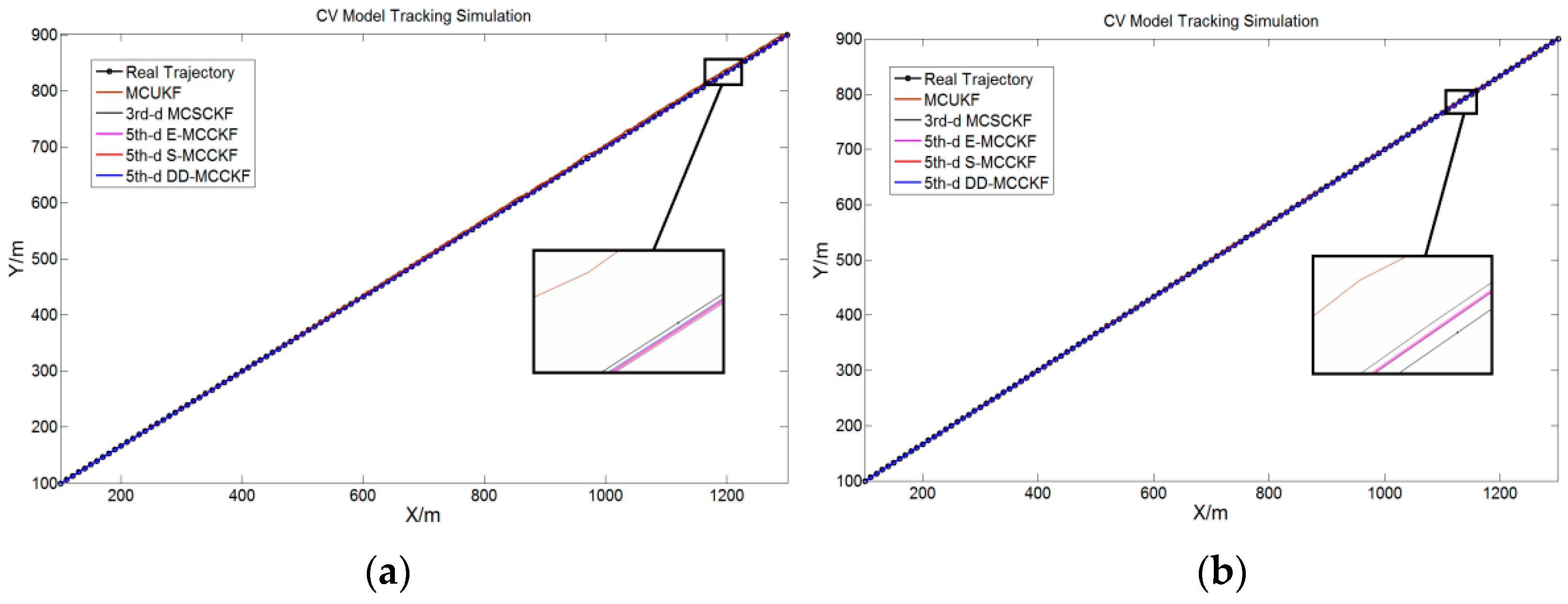
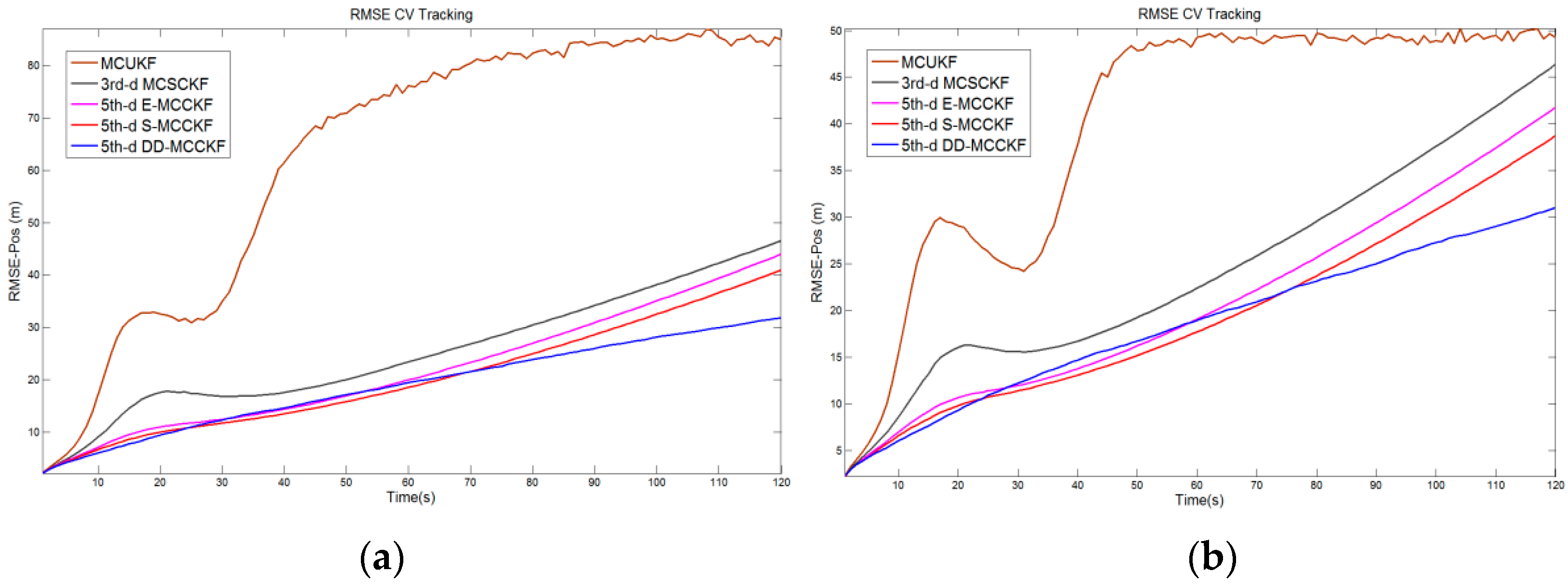
The simulation results are shown in Figure 4, Figure 5 and Figure 6:

The running time of the algorithm was 120 s. The results show that, similar to related properties introduced in Section 2.1, the comprehensive numerical performance of UKF was not as good as that of 3rd-degree CKF, resulting in the highest mean square error and the lowest filtering accuracy of MCUKF. In addition, when n = 4, the number of cubature points used by 5th-degree SCKF and ECKF was the same as those used by the DDKCF proposed in this study. The formula structure was similar. Thus, the calculation amount was very similar. Because DD-CKF maintains the numerical stability when the system dimension is large while calculating with fewer cubature points, and Formula (32) carries out a certain displacement of the coefficient of cubature points to reduce the non-sampling error, the accuracy of DD-MCCKF was slightly higher than that of other algorithms in tracking experiments.

Table 3. Number of points used by different filtering algorithms in Experiment 1, along with the ARMSE for the position and velocity.

Robust Filters	Number of Points	ARMSE Pos (C1, C2)		ARMSE Vel (C1, C2)
MCUKF	2n = 8	63.26	39.98	3.261	2.444
3rd-degree MCSCKF	2n = 8	25.28	24.47	1.496	1.428
5th-degree E-MCCKF	2n2 − 2n + 1 = 25	21.92	20.91	1.432	1.354
5th-degree S-MCCKF	2n2 − 2n + 1 = 25	20.37	19.43	1.401	1.323
(Proposed) 5th-degree DD-MCCKF	2n2 − 2n + 1 = 25	18.96	18.49	1.392	1.320

shows the number of points and ARMSE of each algorithm in Experiment 2 above.

As shown in Table 3, the proposed DD-MCCKF algorithm had the highest estimation accuracy under the premise of using fewer cubature points in a non-Gaussian noise environment.

4.2.2. Simulation Experiment of Robust Filtering Based on Cooperative Turning Tracking Model of Surface Targets

The cooperative turning (CT) model is a coordinate coupling model. In most cases, the coordinate coupling model refers to a turning motion model. Because this type of model is closely related to the coordinates, it can be divided into two types: two-dimensional and three-dimensional turning models. The two-dimensional turning model is also called the planar turning model, that is, the CT model.

The CT model is one of the most important maneuvering models in surface target tracking. It is a commonly used model to describe maneuvering target in USV tracking. The state equation and measurement equation of the CT model are as follows:

$$\{\begin{array}{c}{\mathit{x}}_k=\left(\begin{array}{c}{x}_k\\ {\dot{x}}_k\\ y_k\\ {\dot{y}}_k\\ {\omega }_k\end{array}\right)=\left(\begin{array}{ccccc}1& \frac{\sin \left({\omega }_{k-1}T\right)}{{\omega }_{k-1}}& 0& \frac{\cos \left({\omega }_{k-1}T\right)-1}{{\omega }_{k-1}}& 0\\ 0& \cos \left({\omega }_{k-1}T\right)& 0& -\sin \left({\omega }_{k-1}T\right)& 0\\ 0& \frac{1-\cos \left({\omega }_{k-1}T\right)}{{\omega }_{k-1}}& 1& \frac{\sin \left({\omega }_{k-1}T\right)}{{\omega }_{k-1}}& 0\\ 0& \sin \left({\omega }_{k-1}T\right)& 0& \cos \left({\omega }_{k-1}T\right)& 0\\ 0& 0& 0& 0& 1\end{array}\right)\left(\begin{array}{c}{x}_{k-1}\\ {\dot{x}}_{k-1}\\ y_{k-1}\\ y_{k-1}\\ {\omega }_{k-1}\end{array}\right)+{\mathit{w}}_{k-1}\hfill \\ {\mathit{z}}_k=\left(\begin{array}{c}\sqrt{x_k^2+y_k^2}\\ arctan\left(\frac{y_k-y_l}{x_k-x_l}\right)\end{array}\right)+{\mathit{v}}_k\hfill \end{array},$$

(63)

where $x_k$ is the system state variable, and $x_k,y_k$ and ${\dot{x}}_k{\dot{y}}_k$ represent the position and velocity of the target in the x and y directions, respectively. T represents the sampling period, and ${\omega }_k$ represents the steering angular velocity. $w_k$ represents the process noise, which has covariance matrix $Q_k$, and $v_k$ represents the measurement noise, which has covariance matrix $R_k$. The initial value of the state variable is $x_0$, and the correlation covariance matrix is $P_{0|0}$. To enhance the mobility of the surface target, the parameters were initialized as follows:

$$\begin{array}{l}{\mathit{Q}}_1=q_1^2\left[\begin{array}{ccc}{\mathit{M}}_1& 0& 0\\ 0& {\mathit{M}}_1& 0\\ 0& 0& T_1/3\end{array}\left],{\mathit{Q}}_2=q_2^2\right[\begin{array}{ccc}{\mathit{M}}_2& 0& 0\\ 0& {\mathit{M}}_2& 0\\ 0& 0& T_2/3\end{array}\right]\\ q=0.05,q_1=0.2,q_2=0.3,{\mathit{M}}_k=\left[\begin{array}{cc}{T}_k^3/3& T_k^2/2\\ T_k^2/2& T_k\end{array}\right],T_1=\frac{1}{4},T_2=\frac{1}{6}\\ x_0={\left(100 \mathrm{m},80 \mathrm{m}/\mathrm{s},100 \mathrm{m},120 \mathrm{m}/\mathrm{s},-\frac{8\pi }{180} \mathrm{rad}\right)}^T\\ P_{0|0}=\mathrm{diag}\left(10 {\mathrm{m}}^2,1 {\mathrm{m}}^2/{\mathrm{s}}^2,10 {\mathrm{m}}^2,1 {\mathrm{m}}^2/{\mathrm{s}}^2,0.1 {\mathrm{rad}}^2/{\mathrm{s}}^2\right)\\ R_1=q\mathrm{diag}\left\{{\left(25 \mathrm{m}\right)}^2,{\left(\frac{3\pi }{180}\right)}^2 \mathrm{rad}\right\},R_2=q\mathrm{diag}\left\{{\left(30 \mathrm{m}\right)}^2,{\left(\frac{9\pi }{180}\right)}^2 \mathrm{rad}\right\}\end{array} .$$

(64)

To set up the different types of non-Gaussian state noise and measurement noise environment based on $\{\begin{array}{l}{w}_k~\left(1-\eta \right)N\left(\mathbf{0},Q_1\right)+\eta N\left(\mathbf{0},Q_2\right)\hfill \\ r_k~\left(1-\eta \right)N\left(\mathbf{0},R_1\right)+\eta N\left(\mathbf{0},R_2\right)\hfill \end{array}$, we considered the conditions as follows:

Condition 3.

Under mixture noise,$\eta =\frac{1}{2}$:

$$w_{k3}~\frac{1}{2}{N}_1\left(\mathbf{0},Q_1\right)+\frac{1}{2}{N}_2\left(\mathbf{0},Q_2\right) , r_{k3}~\frac{1}{2}{N}_1\left(\mathbf{0},R_1\right)+\frac{1}{2}{N}_2\left(\mathbf{0},R_2\right) .$$

(65)

Condition 4.

Under mixture noise,$\eta =\frac{2}{3}$:

$$w_{k4}~\frac{1}{3}N\left(\mathbf{0},Q_1\right)+\frac{2}{3}N\left(\mathbf{0},Q_2\right) , r_{k4}~\frac{1}{3}N\left(\mathbf{0},R_1\right)+\frac{2}{3}N\left(\mathbf{0},R_2\right) .$$

(66)

In the simulation experiment, we used the RMSE and ARMSE to evaluate the filtering performance. The RMSE and ARMSE of the displacement, velocity, and steering angle were defined as follows:

$$\begin{array}{c}RMS{E}_{CTpos}=\sqrt{\frac{1}{N}{\displaystyle \sum _{k=1}^N\left[{\left(x_k-{\widehat{x}}_{k|k}\right)}^2+{\left(y_k-{\widehat{y}}_{k|k}\right)}^2\right]}}\hfill \\ RMS{E}_{CTvel}=\sqrt{\frac{1}{N}{\displaystyle \sum _{k=1}^N\left[{\left({\dot{x}}_k-{\widehat{\dot{x}}}_{k|k}\right)}^2+{\left({\dot{y}}_k-{\widehat{\dot{y}}}_{k|k}\right)}^2\right]}}\hfill \\ RMS{E}_{CTomg}=\sqrt{\frac{1}{N}{\displaystyle \sum _{k=1}^N\left[{\left({\omega }_k-{\widehat{\omega }}_{k|k}\right)}^2\right]}}\hfill \\ ARMS{E}_{any}=\frac{1}{A}{\displaystyle \sum _{l=1}^{A}RMS{E}_{any}\left(l\right)}.\hfill \end{array}$$

(67)

Here, N represents the total number of Monte Carlo simulations, and A represents the timestep of each Monte Carlo simulation. In the simulation experiment, We set c in Equations (45) and (46) as 1/3, and we set N = $\mathbf{1}\times {\mathbf{10}}^{\mathbf{5}}$ times and A = 140 s. Lines 1–3 of Equation (67) give the position RMSEs obtained from the real value and estimated value of the position vector and the velocity RMSE and angular-velocity RMSE obtained via the same method as the position RMSE, respectively. Finally, the calculation formula for the ARMSE is presented.

Because the CT model has a strong nonlinearity, and the collaborative CT model can better describe the USV high-speed maneuvering steering process on the water surface in reality than the uniform turning model, this experiment used the CT model to conduct the last robust filtering experiment based on the nonlinear system in a non-Gaussian environment.

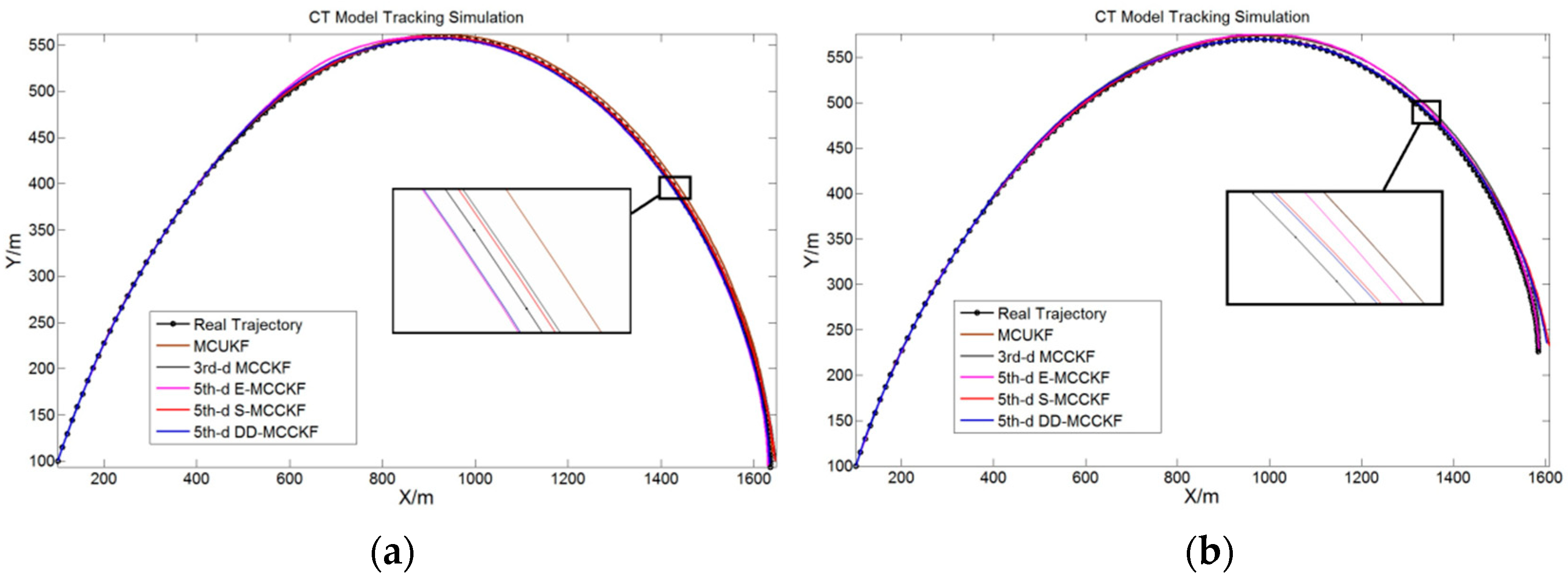
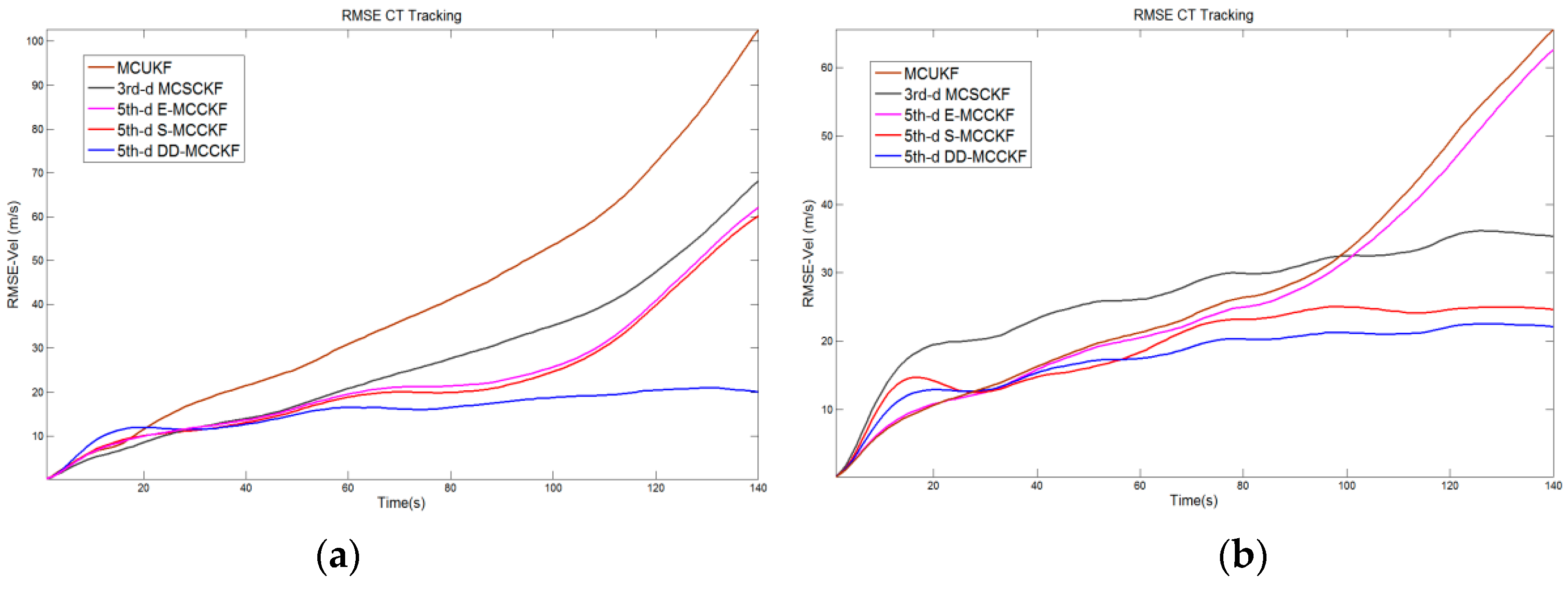
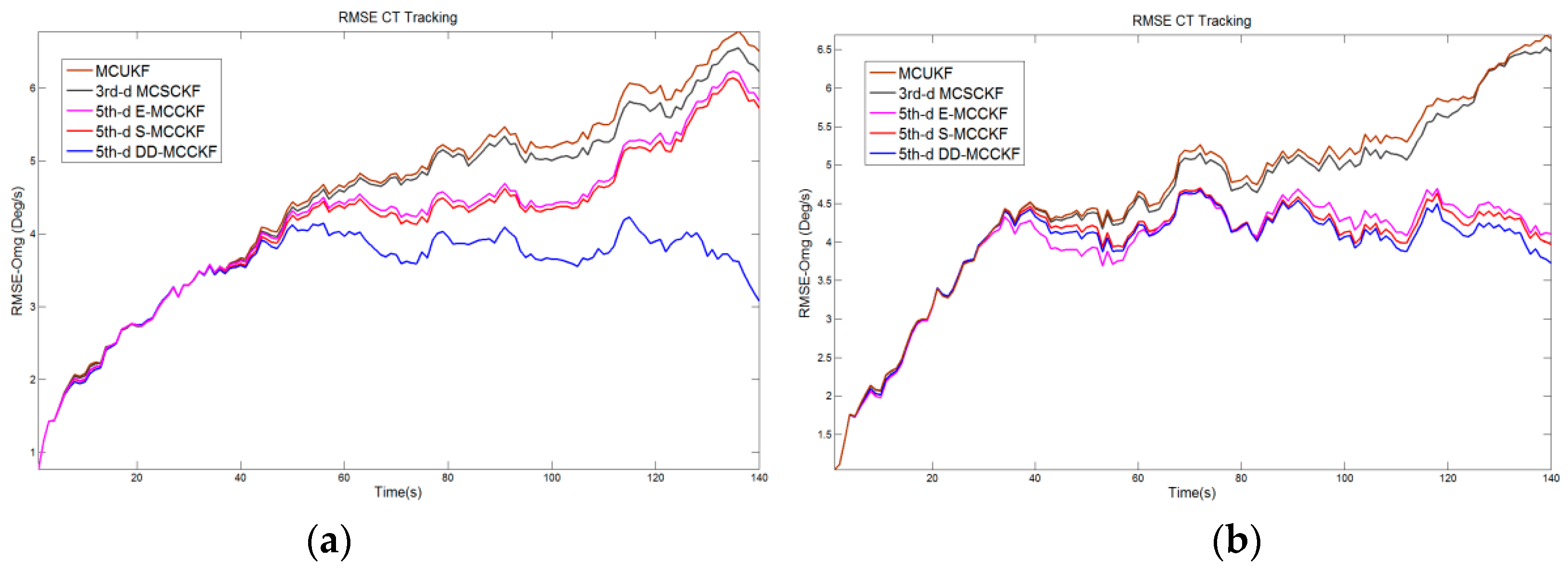
As with Experiment 2 in Section 4.2.1, in the experiment of this section, the robust filter MCUKF proposed in reference [16], the MCSCKF proposed in reference [27] and E-MCCKF and S-MCCKF which are formed by Formula (14), Formula (20) and the MCC method proposed in this paper are used to compare with the robust algorithm DD-MCCKF proposed in this paper in a non-Gaussian state and measured noise environments above. The simulation results for the CT target-tracking model are presented in Figure 7, Figure 8, Figure 9 and Figure 10.

The running time of the algorithm was 140 s. Among the position errors of the simulation results, the accuracy of the MCUKF was the worst owing to the numerical instability and inaccurate UT. Because of the high system dimensions, the approximation process of the ECKF was unstable, and its filtering performance was worse than that of the S-MCCKF. Especially in the position RMSE index, the ECKF was particularly affected by the instability of its formula value, and its filtering accuracy is even lower than that of the 3rd-degree MCCKF.

The DD-MCCKF and S-MCCKF were similar with regard to the structure of the cubature formula and the number of cubature points used. Thus, they had similar filtering accuracies. Because the DD-CKF integrates the two indexes of numerical stability and the number of cubature points used, it is better at improving accuracy and reducing the calculation amount. In addition, the smaller coefficient of the cubature points of the DD-CKF can better reduce non-local sampling problems, which helps further improve its filtering accuracy.

By fine-tuning parameter c in Equations (45) and (46), the non-local sampling problem caused by the increase in the system dimension was alleviated, and the filtering accuracy was increased. For the estimation of the velocity and course angular velocity, the UKF and 3rd-degree CKF had the lowest accuracy, whereas the 5th-degree ECKF and SCKF had similar performance, and the DD-MCCKF had the highest accuracy. Furthermore, as indicated in

Table 4. Number of points and the ARMSEs of the position, velocity and course angular velocity for different robust filtering algorithms in the target tracking simulation of Experiment 4.2.2.

Robust Filters	Number of Points	ARMSE Pos-C1	ARMSE Pos-C2	ARMSE Vel-C1	ARMSE Vel-C2	ARMSE Omg-C1	ARMSE Omg-C2
MCUKF	2n = 10	10.41	18.84	40.38	27.29	4.532	4.613
3rd-degree MCSCKF	2n= 10	11.78	14.66	26.88	26.07	4.430	4.539
5th-degree E-MCCKF	2n2 + 1 = 51	9.824	15.17	23.29	26.63	4.143	3.923
5th-degree S-MCCKF	2n2 + 1 = 51	8.456	13.78	22.47	19.21	4.087	3.931
(Proposed) 5th-degree DD-MCCKF	2n2 + 1 = 51	5.956	11.85	15.50	17.42	3.492	3.869

, the ARMSEs obtained via the proposed algorithm were lower than those for the 5th-degree ECKF and SCKF.

5. Conclusions

A high-degree robust CKF algorithm, based on a new cubature formula and MCC, was developed. First, according to the construction method of the fully symmetric cubature formula, different cubature-point coordinate generators were used to construct a new high-degree cubature formula and fine-tune its parameters to increase its accuracy. Subsequently, a new robust cost function was constructed by combining the MCC and WLS methods.

As a statistical measure of the similarity between random variables, MCC can extract information from all even moments under the appropriate kernel bandwidth. This helped us make better use of the higher-order moment information of the signal. Therefore, in filtering applications, MCC is more robust to non-Gaussian mixture noise than the conventional nonlinear Kalman filter, which can only use second-order information. The fixed-point iteration solution of the equation was embedded in the nonlinear Kalman filtering process to obtain a robust filtering algorithm. Finally, a new high-degree robust CKF algorithm was obtained by combining the new estimation process with the KF framework. The aim was to use as few cubature coordinate points as possible to achieve the highest filtering accuracy and stability in a non-Gaussian noise environment. The proposed method was applied to the target tracking of an unmanned surface vessel. The simulation experiment exhibited a smaller number of computations, higher filtering accuracy, and better numerical stability when compared to (or similar results to) other algorithms of the same order.

The new-proposed filter probably has a certain application value in practical application scenarios, such as the course tracking of unmanned surface vessels, tracking for maritime moving targets or surface vessel rescuing, and in the sea area with strong environmental interference (e.g., wind and waves). The autonomous navigation target of obstacle avoidance on the water surface may be achieved under the condition of large errors in sensor distance and angle measurement. However, owing to the uncertainty and complexity of the surface environment, the measurement process based on sensors and satellite positioning may be affected or temporarily unavailable. At the same time, some state estimation problems in more complex environments are also the focus of research, such as estimation with bias compensation, nonlinear filtering based on state constraints, robust constraints, state estimation in complex domain impulsive noise etc. As mentioned in References [28,29,30,31,32,33,34,35,36,37,38,39,40,41,42,43,44,45]. These issues need to be further studied in the following work.

References

1. Venkateswarlu, C.; Avantika, S. Optimal state estimation of multicomponent batch distillation. Chem. Eng. Sci. 2001, 56, 5771–5786. [Google Scholar] [CrossRef]
2. Ito, M.; Tsujimichi, S.; Kosuge, Y. Tracking a three-dimensional moving target with distributed passive sensors using extended Kalman filter. Electron. Commun. Jpn. 2010, 84, 74–85. [Google Scholar] [CrossRef]
3. Bucy, R.S.; Senne, K.D. Digital synthesis of non-linear filters. Automatica 1971, 7, 287–298. [Google Scholar] [CrossRef]
4. Julier, S.J.; Uhlmann, J.K. A new extension of the Kalman filter to nonlinear systems. In AeroSense: The Ilth International Symposium on Aerospace/Defense Sensing, Simulation and Controls; SPIE: New York, NY, USA, 1997; pp. 182–193. [Google Scholar]
5. Julier, S.J.; Uhlmann, J.K. Unscented filtering and nonlinear estimation. Proc. IEEE 2004, 92, 401–422. [Google Scholar] [CrossRef]
6. Arasaratnam, I.; Haykin, S. Cubature Kalman filters. IEEE Trans. Autom. Control 2009, 54, 1254–1269. [Google Scholar] [CrossRef]
7. Norgaard, M.; Poulsen, N.K.; Ravn, O. New developments in state estimation for nonlinear systems. Automatica 2000, 36, 1627–1638. [Google Scholar] [CrossRef]
8. Ito, K.; Xiong, K. Gaussian filters for nonlinear filtering problems. IEEE Trans. Autom. Control 2000, 45, 910–927. [Google Scholar] [CrossRef]
9. Arasaratnam, I.; Haykin, S.; Hurd, T.R. Cubature Kalman Filtering for Continuous-Discrete Systems: Theory and Simulations. IEEE Trans. Signal Processing 2010, 58, 4977–4993. [Google Scholar] [CrossRef]
10. Jia, B.; Xin, M.; Cheng, Y. High-degree cubature Kalman filter. Automatica 2013, 49, 510–518. [Google Scholar] [CrossRef]
11. Meng, D.; Miao, L.; Shao, H.; Shen, J. A Seventh-Degree Cubature Kalman Filter. Asian J. Control 2018, 20, 250–262. [Google Scholar] [CrossRef]
12. Zhang, X. Cubature Information Filters Using High-Degree and Embedded Cubature Rules. Circuits Syst. Signal. Processing 2014, 33, 1799–1818. [Google Scholar] [CrossRef]
13. McNamee, J.; Stenger, F. Construction of fully symmetric numerical integration formulas of fully symmetric numerical integration formulas. Numer. Math. 1967, 10, 327–344. [Google Scholar] [CrossRef]
14. Izanloo, R.; Fakoorian, S.A.; Yazdi, H.S.; Simon, D. Kalman filtering based on the maximum correntropy criterion in the presence of non-Gaussian noise. In Proceedings of the 2016 Annual Conference on Information Science and Systems (CISS), Princeton, NJ, USA, 16–18 March 2016. [Google Scholar]
15. Terejanu, G.; Singla, P.; Singh, T.; Scott, P.D. Adaptive Gaussian Sum Filter for Nonlinear Bayesian Estimation. IEEE Trans. Autom. Control 2011, 56, 2151–2156. [Google Scholar] [CrossRef]
16. Wang, G.; Li, N.; Zhang, Y. Maximum correntropy unscented Kalman and information filters for non-Gaussian measurement noise. J. Frankl. Inst. 2017, 354, 8659–8677. [Google Scholar] [CrossRef]
17. Meng, Q.; Li, X. Minimum Cauchy Kernel Loss Based Robust Cubature Kalman Filter and Its Low Complexity Cost Version With Application on INS/OD Integrated Navigation System. IEEE Sens. J. 2022, 22, 9534–9542. [Google Scholar] [CrossRef]
18. He, J.; Sun, C.; Zhang, B.; Wang, P. Variational Bayesian-Based Maximum Correntropy Cubature Kalman Filter With Both Adaptivity and Robustness. IEEE Sens. J. 2020, 21, 1982–1992. [Google Scholar] [CrossRef]
19. Zhao, L.; Wang, J.; Yu, T.; Chen, K.; Su, A. Incorporating delayed measurements in an improved high-degree cubature Kalman filter for the nonlinear state estimation of chemical processes. ISA Trans. 2019, 86, 122–133. [Google Scholar] [CrossRef] [PubMed]
20. Santos-León, C.; Orive, R.; Acosta, D.; Acosta, L. The Cubature Kalman Filter revisited. Automatica 2021, 127, 109541. [Google Scholar] [CrossRef]
21. Stroud, A.H. Approximate Calculation of Multiple Integrals. In Englewood Cliffs; Prentice Hall: Hoboken, NJ, USA, 1971. [Google Scholar]
22. Stroud, A.H.; Secrest, D. Approximate integration formulas for certain spherically symmetric regions. Math. Comput. 1963, 17, 105–135. [Google Scholar] [CrossRef]
23. Mysovskikh, I.P. The Approximation of Multiple Integrals by Using Interpolatory Cubature Formulae; DeVore, R.A., Scherer, K., Eds.; Quantitative Approximation Academic Press: New York, NY, USA, 1980; pp. 217–243. [Google Scholar]
24. Lu, J.; Darmofal, D.L. Higher-Dimensional Integration with Gaussian Weight for Applications in Probabilistic Design. Siam J. Sci. Comput. 2008, 26, 613–624. [Google Scholar] [CrossRef]
25. Wang, G.; Li, N.; Zhang, Y. Hybrid consensus sigma point approximation nonlinear filter using statistical linearization. Trans. Inst. Measur. Control. 2017. [Google Scholar] [CrossRef]
26. Horn, R.A.; Johnson, C.R. Matrix Analysis, 2nd ed.; Cambridage University Press: Cambridge, UK, 2013. [Google Scholar]
27. He, J.; Sun, C.; Zhang, B.; Wang, P. Maximum Correntropy Square-Root Cubature Kalman Filter for Non-Gaussian Measurement Noise. IEEE Access 2020, 8, 70162–70170. [Google Scholar] [CrossRef]
28. Wang, Y.; Wang, H.; Li, Q.; Xiao, Y.; Ban, X. Passive Sonar Target Tracking Based on Deep Learning. J. Mar. Sci. Eng. 2022, 10, 181. [Google Scholar] [CrossRef]
29. Wang, X.; Liang, Y.; Pan, Q.; Zhao, C. Gaussian filter for nonlinear systems with one-step randomly delayed measurements. Automatica 2013, 49, 976–986. [Google Scholar] [CrossRef]
30. Ho, Y.C.; Lee, R.C.K.A. A Bayesian approach to problems in stochastic estimation and control. IEEE Trans. Autom. Control 1964, 9, 333–339. [Google Scholar] [CrossRef]
31. Liu, D.; Zhao, H. Bias-compensated subband adaptive filter algorithm based on maximum correntropy criterion. In Proceedings of the 2021 IEEE 16th Conference on Industrial Electronics and Applications (ICIEA), Chengdu, China, 1–4 August 2021; pp. 1202–1206. [Google Scholar] [CrossRef]
32. Xiang, W.; Zhao, H. Robust Filtering of Affine-Projection-Like Maximum Correntropy Algorithm with Bias-Compensated. In Proceedings of the 2021 IEEE 16th Conference on Industrial Electronics and Applications (ICIEA), Chengdu, China, 1–4 August 2021; pp. 1207–1210. [Google Scholar] [CrossRef]
33. Feng, X.; Feng, Y.; Zhou, F.; Ma, L.; Yang, C.-X. Nonlinear Non-Gaussian Estimation Using Maximum Correntropy Square Root Cubature Information Filtering. IEEE Access 2020, 8, 181930–181942. [Google Scholar] [CrossRef]
34. Merabti, H.; Massicotte, D.; Zhu, W.-P. Nonlinearity-Robust Linear Acoustic Echo Canceller Using the Maximum Correntropy Criterion. In Proceedings of the 2019 IEEE International Symposium on Signal Processing and Information Technology (ISSPIT), Ajman, United Arab Emirates, 10–12 December 2019; pp. 1–5. [Google Scholar] [CrossRef]
35. Zou, Y.; Zou, S.; Tang, X.; Yu, L. Maximum Correntropy Criterion Kalman Filter Based Target Tracking with State Constraints. In Proceedings of the 2020 39th Chinese Control Conference (CCC), Shenyang, China, 27–29 July 2020; pp. 3505–3510. [Google Scholar] [CrossRef]
36. Liu, X.; Ren, Z.; Lyu, H.; Jiang, Z.; Ren, P.; Chen, B. Linear and Nonlinear Regression-Based Maximum Correntropy Extended Kalman Filtering. IEEE Trans. Syst. Man Cybern. Syst. 2021, 51, 3093–3102. [Google Scholar] [CrossRef]
37. Chen, S.; Zhang, Q.; Zhang, T.; Zhang, L.; Peng, L.; Wang, S. Robust State Estimation With Maximum Correntropy Rotating Geometric Unscented Kalman Filter. IEEE Trans. Instrum. Meas. 2022, 71, 1–14. [Google Scholar] [CrossRef]
38. Bhattacharjee, S.S.; Shaikh, M.A.; Kumar, K.; George, V.N. Robust Constrained Generalized Correntropy and Maximum Versoria Criterion Adaptive Filters. IEEE Trans. Circuits Syst. II Express Briefs 2021, 68, 3002–3006. [Google Scholar] [CrossRef]
39. Zhang, X.; Tian, Y.; Han, X.; Liu, Q.; Guo, L. Maximum Correntropy Criterion based Sparse Channel Estimation under Impulsive Noise in Complex Domain. In Proceedings of the 2019 IEEE International Conference on Signal, Information and Data Processing (ICSIDP), Chongqing, China, 11–13 December 2019; pp. 1–5. [Google Scholar] [CrossRef]
40. Cheng, L.; Wang, K.; Ren, M.; Yan, G. Adaptive Filter Approach for GPS Multipath Estimation Under Correntropy Criterion in Dynamic Multipath Environment. IEEE Trans. Signal Processing 2019, 67, 5798–5810. [Google Scholar] [CrossRef]
41. Fakoorian, S.; Izanloo, R.; Shamshirgaran, A.; Simon, D. Maximum Correntropy Criterion Kalman Filter with Adaptive Kernel Size. In Proceedings of the 2019 IEEE National Aerospace and Electronics Conference (NAECON), Dayton, OH, USA, 15–19 July 2019; pp. 581–584. [Google Scholar] [CrossRef]
42. Song, H.; Ding, D.; Dong, H.; Han, Q.-L. Distributed Maximum Correntropy Filtering for Stochastic Nonlinear Systems Under Deception Attacks. IEEE Trans. Cybern. 2022, 52, 3733–3744. [Google Scholar] [CrossRef] [PubMed]
43. Chu, L.; Li, W. Fusion-based multi-kernel learning filter with maximum correntropy criterion. In Proceedings of the 2020 IEEE 9th Data Driven Control and Learning Systems Conference (DDCLS), Liuzhou, China, 20–22 November 2020; pp. 556–561. [Google Scholar] [CrossRef]
44. Li, W.; Xiong, K.; Liu, Y. Diffusion Kalman filter by using maximum correntropy criterion. In Proceedings of the 2019 12th Asian Control Conference (ASCC), Kitakyushu, Japan, 9–12 June 2019; pp. 203–208. [Google Scholar]
45. Kulikova, M.V. Square-Root Approach for Chandrasekhar-Based Maximum Correntropy Kalman Filtering. IEEE Signal Processing Lett. 2019, 26, 1803–1807. [Google Scholar] [CrossRef]
Figure 1. RMSE for different filters in Experiment 4.1.1.
Jmse 10 01070 g001
Figure 2. Tracking trajectory of the 3rd-drgree CKF and the 3rd-degree MCCKF under non-Gaussian noise conditions in Equation (61).
Jmse 10 01070 g002
Figure 3. RMSE of the position and velocity for different filters under non-Gaussian noise conditions in Equation (61) ((a) is the position RMSE and (b) is the velocity RMSE).
Jmse 10 01070 g003
Figure 4. Tracking trajectories of a surface target (unmanned surface vessel) under non-Gaussian noise conditions ((a) is the result under Equation (61) and (b) is the result under Equation (62)).
Jmse 10 01070 g004
Figure 5. Position RMSEs of robust target-tracking algorithms under non-Gaussian noise conditions ((a) is the result under Equation (61) and (b) is the result under Equation (62)).
Jmse 10 01070 g005
Figure 6. Velocity RMSEs of robust target-tracking algorithms under non-Gaussian noise conditions ((a) is the result under Equation (61) and (b) is the result under Equation (62)).
Jmse 10 01070 g006
Figure 7. Tracking trajectories of surface target (unmanned surface vessel) under non-Gaussian noise conditions ((a) is the result under Equation (65) and (b) is the result under Equation (66)).
Jmse 10 01070 g007
Figure 8. Position RMSEs of robust target-tracking algorithms under non-Gaussian noise conditions ((a) is the result under Equation (65) and (b) is the result under Equation (66)).
Jmse 10 01070 g008
Figure 9. Velocity RMSEs of robust target-tracking algorithms under non-Gaussian noise conditions ((a) is the result under Equation (65) and (b) is the result under Equation (66)).
Jmse 10 01070 g009
Figure 10. Course angular-velocity RMSEs of robust target-tracking algorithms under non-Gaussian noise conditions ((a) is the result under Equation (65) and (b) is the result under Equation (66)).
Jmse 10 01070 g010