
The Seabed Makes the Dolphins: Physiographic Features Shape the Size and Structure of the Bottlenose Dolphin Geographical Units

 , ,
, ,  , ,
, , 
 , ,
, ,
Abstract
1. Introduction
2. Material and Methods
2.1. Study Areas
2.1.1. Alboran Sea
2.1.2. Gulf of Lion
2.1.3. Pelagos Sanctuary
2.1.4. Gulf of Ambracia
2.2. Data Collection
2.3. Data Analysis
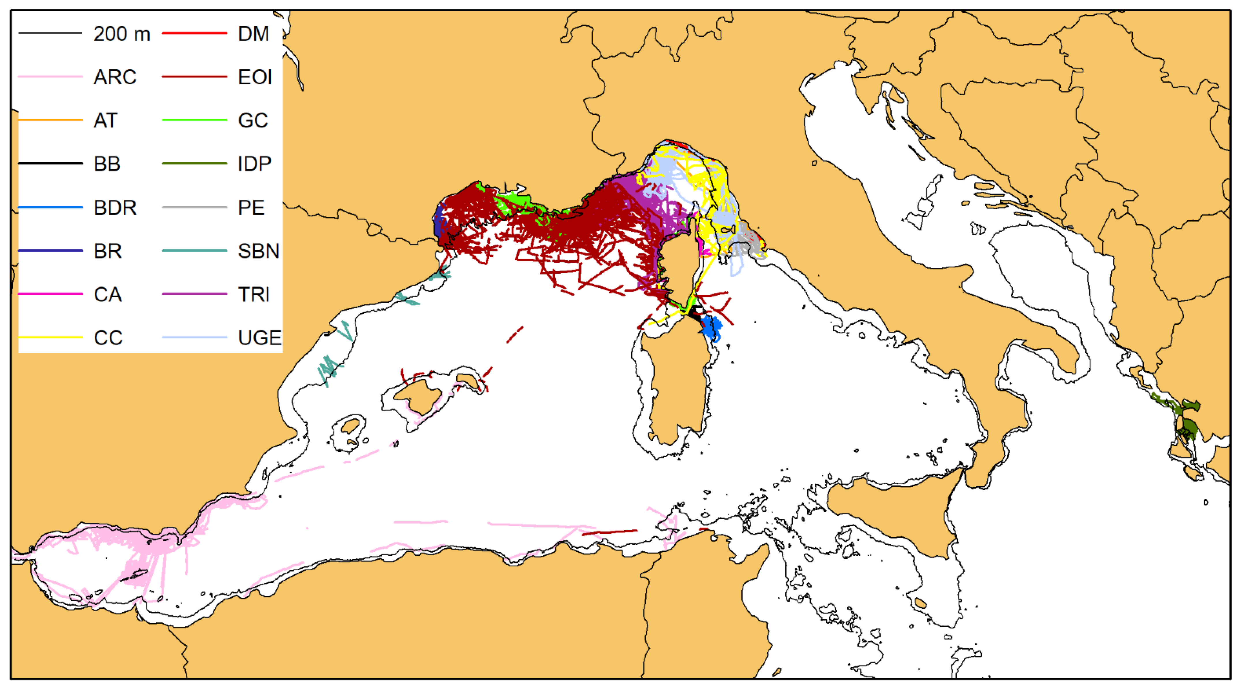
2.3.1. Distribution
2.3.2. Photographic Data and Matching Process
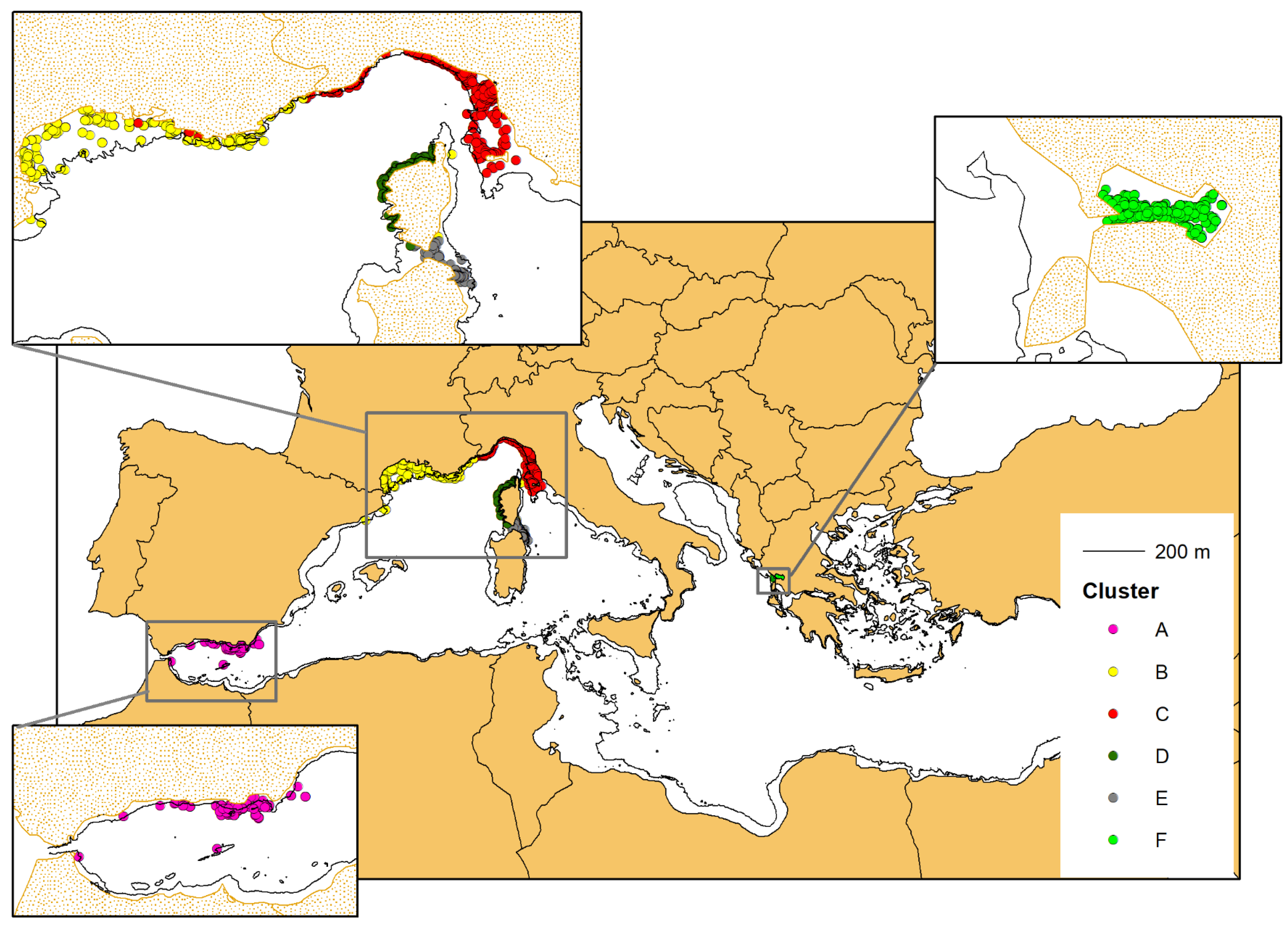
2.3.3. Connectivity Analysis and Cluster Identification
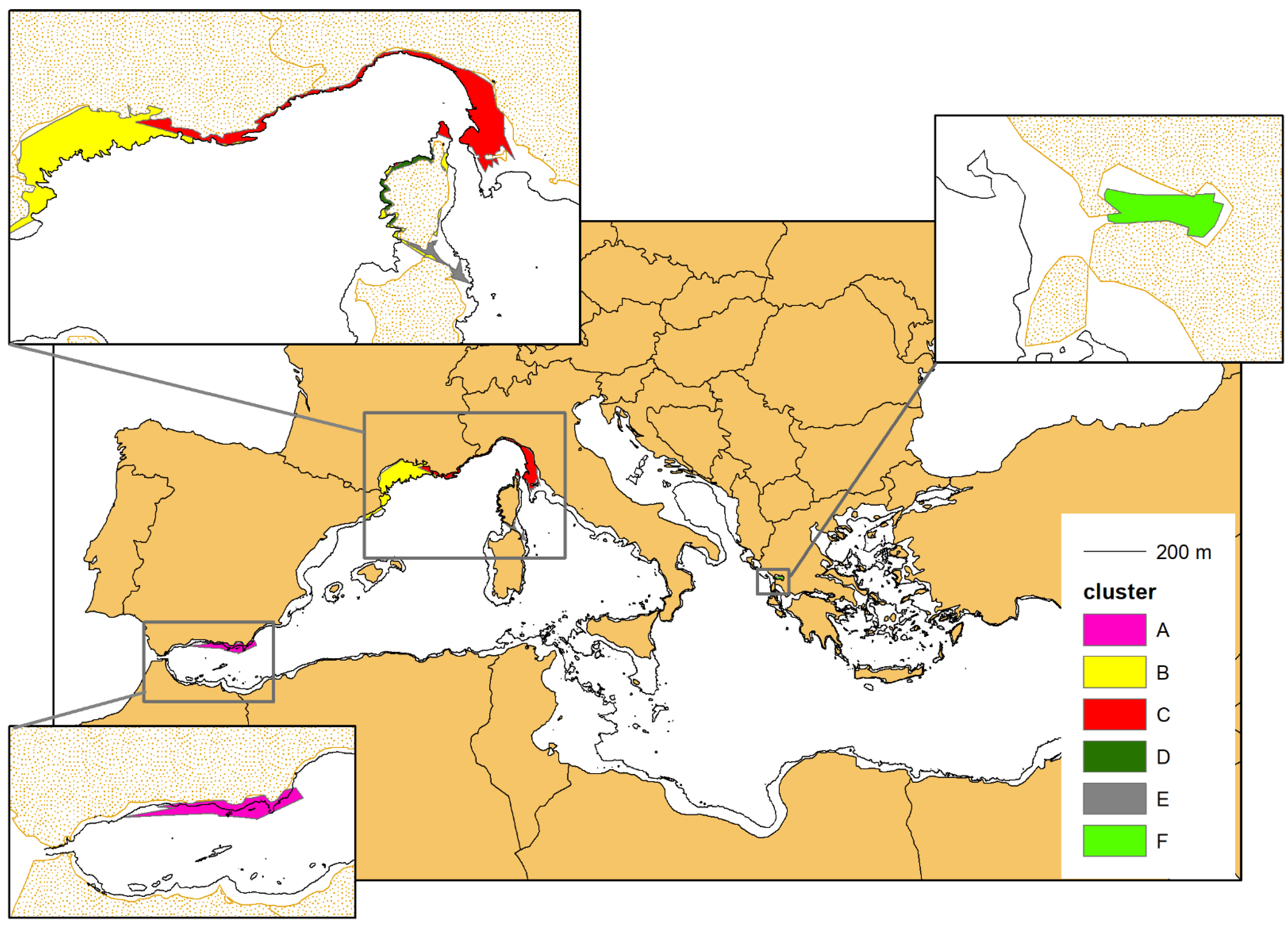
2.3.4. Mapping the Different Geographical Units
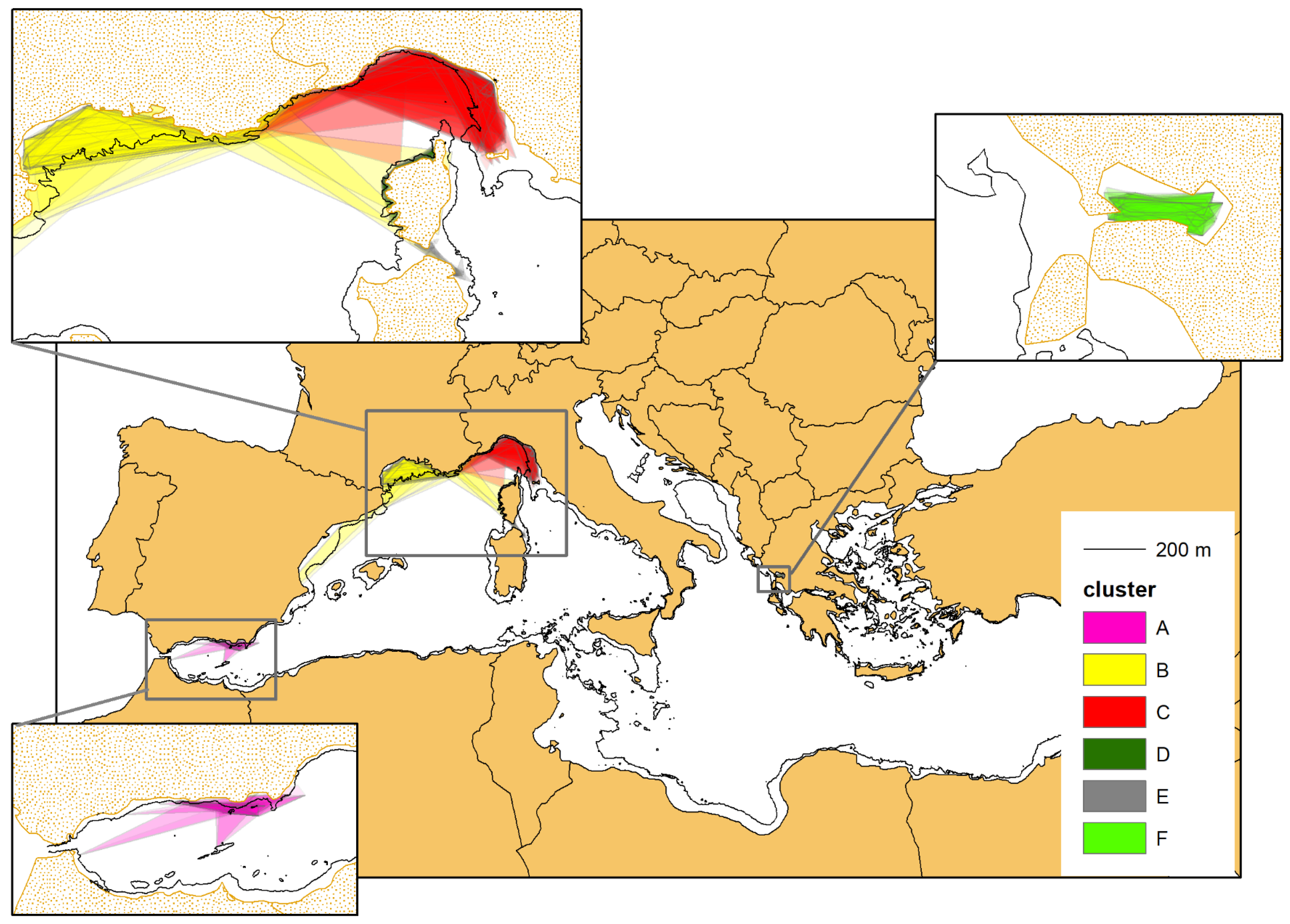
2.3.5. Movement Analysis through Minimum Convex Polygon (MCP)
2.3.6. Group Size
2.3.7. Abundance Estimates and Density
3. Results
3.1. Distribution
3.2. Photographic Data and Matching Process
3.3. Connectivity Analysis and Cluster Identification
3.4. Mapping the Different Geographical Units
3.5. Movement Analysis through Minimum Convex Polygon (MCP)
3.6. Group Size
3.7. Abundance Estimates and Density
4. Discussion and Conclusions
Author Contributions
Funding
Institutional Review Board Statement
Informed Consent Statement
Data Availability Statement
Acknowledgments
Conflicts of Interest
References
- Shane, S.H.; Wells, R.S.; Würsig, B. Ecology, behavior and social organization of the bottlenose dolphin: A review. Mar. Mammal Sci. 1986, 2, 34–63. [Google Scholar] [CrossRef]
- Rice, D.W. Marine Mammals of the World: Systematics and Distribution; The Society for Marine Mammology: San Diego, CA, USA, 1998. [Google Scholar]
- Wells, R.S.; Scott, M.D. Bottlenose dolphin Tursiops truncatus (Montagu, 1821). In Handbook of Marine Mammals, Volume VI.; The Second Book of Dolphins and Porpoises; Ridgway, S.H., Harrison, R., Eds.; Academic Press: San Diego, CA, USA, 1999; pp. 137–182. [Google Scholar]
- Wells, R.S.; Scott, M.D. Common Bottlenose Dolphin: Tursiops truncatus. In Encyclopedia of Marine Mammals; Academic Press: San Diego, CA, USA, 2009; pp. 249–255. [Google Scholar]
- Wells, R.S.; Scott, M.D. Bottlenose dolphin, Tursiops truncatus, common bottlenose dolphin. In Encyclopedia of Marine Mammals; Academic Press: San Diego, CA, USA, 2018; pp. 118–125. [Google Scholar]
- Walker, W.A. Geographic variation in morphology and biology of bottlenose dolphins (Tursiops truncatus) in the eastern North Pacific. NOAA/NMFS Southwest Fisheries Science Centre, Administrative Report No. LJ-81-3C. Available online: https://repository.library.noaa.gov/view/noaa/22873 (accessed on 10 May 2022).
- Van Waerebeek, K.; Reyes, J.C.; Read, A.J.; McKinnon, J. Preliminary observation of bottlenose dolphins from the Pacific coast of South America. In The Bottlenose Dolphin; Leatherwood, S., Reeves, R.R., Eds.; Academic Press: San Diego, CA, USA, 1990; pp. 143–154. [Google Scholar]
- Hoelzel, A.R.; Potter, C.W.; Best, P.B. Genetic differentiation between parapatric ‘nearshore’ and ‘offshore’ populations of the bottlenose dolphin. Proc. R Soc. B 1998, 265, 1177–1183. [Google Scholar] [CrossRef] [PubMed]
- Torres, L.G.; Rosel, P.E.; D’Agrosa, C.; Read, A.J. Improving management of overlapping bottlenose dolphin ecotypes through spatial analysis and genetics. Mar. Mammal Sci. 2003, 19, 502–514. [Google Scholar] [CrossRef]
- Parsons, K.M.; Durban, J.W.; Claridge, D.E.; Herzing, D.L.; Balcomb, K.C.; Noble, L.R. Population genetic structure of coastal bottlenose dolphins (Tursiops truncatus) in the Northern Bahamas. Mar. Mammal Sci. 2006, 22, 276–298. [Google Scholar] [CrossRef]
- Tezanos-Pinto, G.; Baker, C.S.; Russell, K.; Martien, K.; Baird, R.W.; Hutt, A.; Stone, G.; Mignucci-Giannoni, A.A.; Caballero, S.; Endo, T.; et al. A worldwide perspective on the population structure and genetic diversity of bottlenose dolphins (Tursiops truncatus) in New Zealand. J. Hered. 2008, 100, 11–24. [Google Scholar] [CrossRef]
- Mirimin, L.; Miller, R.; Dillane, E.; Berrow, S.D.; Ingram, S.; Cross, T.F.; Rogan, E. Fine-scale population genetic structuring of bottlenose dolphins in Irish coastal waters. Anim. Conserv. 2011, 14, 342–353. [Google Scholar] [CrossRef]
- Perrin, W.F.; Thieleking, J.L.; Walker, W.A.; Archer, F.I.; Robertson, K.M. Common bottlenose dolphins (Tursiops truncatus) in California waters: Cranial differentiation of coastal and offshore ecotypes. Mar. Mammal Sci. 2011, 27, 769–792. [Google Scholar] [CrossRef]
- Louis, M.; Viricel, A.; Lucas, T.; Peltier, H.; Alfonsi, E.; Berrow, S.; Brownlow, A.; Covelo, P.; Dabin, W.; Deaville, R.; et al. Habitat-driven population structure of bottlenose dolphins, Tursiops truncatus, in the North-East Atlantic. Mol. Ecol. 2014, 23, 857–874. [Google Scholar] [CrossRef] [PubMed]
- Louis, M.; Galimberti, M.; Archer, F.; Berrow, S.; Brownlow, A.; Fallon, R.; Nykänen, M.; O’brien, J.; Robertson, K.M.; Rosel, P.E.; et al. selection on ancestral genetic variation fuels repeated ecotype formation in bottlenose dolphins. Sci. Adv. 2021, 7, eabg1245. [Google Scholar] [CrossRef] [PubMed]
- Oudejans, M.G.; Visser, F.; Englund, A.; Rogan, E.; Ingram, S.N. Evidence for Distinct Coastal and Offshore Communities of Bottlenose Dolphins in the North East Atlantic. PLoS ONE 2015, 10, e0122668. [Google Scholar] [CrossRef]
- Chen, I.; Nishida, S.; Yang, W.-C.; Isobe, T.; Tajima, Y.; Rus Hoelzel, A. Genetic diversity of bottlenose dolphin (Tursiops sp.) populations in the western North Pacific and the conservation implications. Mar. Biol. 2017, 164, 202. [Google Scholar] [CrossRef] [PubMed]
- Fruet, P.F.; Secchi, E.R.; Di Tullio, J.C.; Simões-Lopes, P.C.; Daura-Jorge, F.; Costa, A.P.; Vermeulen, E.; Flores, P.A.C.; Genoves, R.C.; Laporta, P.; et al. Genetic divergence between two phenotypically distinct bottlenose dolphin ecotypes suggests separate evolutionary trajectories. Ecol. Evol. 2017, 7, 9131–9143. [Google Scholar] [CrossRef] [PubMed]
- de los Bayas-Rea, R.Á.; Félix, F.; Montufar, R. Genetic divergence and fine scale population structure of the common bottlenose dolphin (Tursiops truncatus) found in the Gulf of Guayaquil, Ecuador. PeerJ 2018, 6, e4589. [Google Scholar] [CrossRef]
- Segura-García, I.; Rojo-Arreola, L.; Rocha-Olivares, A.; Heckel, G.; Gallo-Reynoso, J.P.; Hoelzel, R. Eco-Evolutionary Processes Generating Diversity Among Bottlenose Dolphin, Tursiops truncatus, Populations off Baja California, Mexico. Evol. Biol. 2018, 45, 223–236. [Google Scholar] [CrossRef]
- Louis, M.; Buanic, M.; Lefeuvre, C.; Le Nilliot, P.; Ridoux, V.; Spitz, J. Strong bonds and small home range in a resident bottlenose dolphin community in a Marine Protected Area (Britanny, France, Northeast Atlantic). Mar. Mammal Sci. 2017, 33, 1194–1203. [Google Scholar] [CrossRef]
- Rako-Gospić, N.; Radulović, M.; Vučur, T.; Pleslić, G.; Holcer, D.; Mackelworth, P. Factor associated variations in the home range of a resident Adriatic common bottlenose dolphin population. Mar. Pollut. Bull. 2017, 124, 234–244. [Google Scholar] [CrossRef] [PubMed]
- Holcer, D. Ecology of the Common Bottlenose Dolphin, Tursiops truncatus (Montagu, 1821) in the Central Adriatic Sea. Ph.D. Thesis, University of Zagreb, Zagreb, Croatia, 2012. [Google Scholar]
- Defran, R.H.; Weller, D.W.; Kelly, D.L.; Espinosa, M.A. Range characteristics of Pacific coast bottlenose dolphins (Tursiops truncatus) in the Southern California bight. Mar. Mammal Sci. 1999, 15, 381–393. [Google Scholar] [CrossRef]
- Ballance, L.T. Habitat use patterns and ranges of the bottlenose dolphin in the Gulf of California, Mexico. Mar. Mammal Sci. 1992, 8, 262–274. [Google Scholar] [CrossRef]
- Scott, M.D.; Wells, R.S.; Irvine, A.B. A long-term study of bottlenose dolphins on the west coast of florida. In The Bottlenose Dolphin; Leatherwood, S., Reeves, R.R., Eds.; Academic press: San Diego, CA, USA, 1990; pp. 235–244. [Google Scholar]
- Pilleri, G.; Gihr, M. Uber adriatische Tursiops truncatus (Montagu, 1821) und vergleichende Untersuchungen über mediterrane und atlantische Tümmler. Investig. Cetaceans 1969, 1, 66–73. [Google Scholar]
- Cagnolaro, L.; Di Natale, A.; Notarbartolo di Sciara, G.C. Guide per il Riconoscimento Delle Specie Animali Delle Acque Lagunari e Costiere Italiane. AQ/1/224, 9; Consiglio Nazionale delle Ricerche: Genova, Italy, 1983. [Google Scholar]
- Notarbartolo di Sciara, G.; Demma, M. Guida dei Mammiferi Marini del Mediterraneo; Franco Muzzio Editore: Padova, Italy, 1994. [Google Scholar]
- Bearzi, G.; Fortuna, C.; Reeves, R.R. Ecology and conservation of common bottlenose dolphins Tursiops truncatus in the Mediterranean Sea. Mammal Rev. 2009, 39, 92–123. [Google Scholar] [CrossRef]
- Notarbartolo di Sciara, G. Marine Mammals in the Mediterranean Sea: An Overview. Adv. Mar. Biol. 2016, 75, 1–36. [Google Scholar] [PubMed]
- Cañadas, A.; Sagarminaga, R.; Garcia-Tiscar, S. Cetacean distribution related with depth and slope in the Mediterranean waters off southern Spain. Deep. Sea Res. 2002, 49, 2053–2073. [Google Scholar] [CrossRef]
- Cañadas, A.; Sagarminaga, R.; De Stephanis, R.; Urquiola, E.; Hammond, P.S. Habitat preference modelling as a conservation tool: Proposals for marine protected areas for cetaceans in southern Spanish waters. Aquat. Conserv. Mar. Freshw. Ecosyst. 2005, 15, 495–521. [Google Scholar] [CrossRef]
- Gaspari, S.; Scheinin, A.; Holcer, D.; Fortuna, C.; Natali, C.; Genov, T.; Frantzis, A.; Chelazzi, G.; Moura, A.E. Drivers of Population Structure of the Bottlenose Dolphin (Tursiops truncatus) in the Eastern Mediterranean Sea. Evol. Biol. 2015, 42, 177–190. [Google Scholar] [CrossRef]
- Gnone, G.; Bellingeri, M.; Paraboschi, M.; Campana, I.; Alessi, J.; Nuti, S.; Salvioli, F.; Tepsich, P.; Rosso, M.; Moulins, A.; et al. TursioMed: Final Scientific Report. The final scientific report of the TursioMed project, funded by Blue Planet Virginia Böger Stiftung X.X. 2021; Unpublished work. [Google Scholar]
- Moura, A.E.; Shreves, K.; Pilot, M.; Andrews, K.R.; Moore, D.M.; Kishida, T.; Möller, L.; Natoli, A.; Gaspari, S.; McGowen, M.; et al. Phylogenomics of the genus Tursiops and closely related Delphininae reveals extensive reticulation among lineages and provides inference about eco-evolutionary drivers. Mol. Phylogenet. Evol. 2020, 146, 106756. [Google Scholar] [CrossRef]
- Gnone, G.; Bellingeri, M.; Dhermain, F.; Dupraz, F.; Nuti, S.; Bedocchi, D.; Moulins, A.; Rosso, M.; Alessi, J.; McCrea, R.S.; et al. Distribution, abundance, and movements of the bottlenose dolphin (Tursiops truncatus) in the Pelagos Sanctuary MPA (north-west Mediterranean Sea). Aquat. Conserv. Mar. Freshw. Ecosyst. 2011, 21, 372–388. [Google Scholar] [CrossRef]
- Carnabuci, M.; Schiavon, G.; Bellingeri, M.; Fossa, F.; Paoli, C.; Vassallo, P.; Gnone, G. Connectivity in the network macrostructure of Tursiops truncatus in the Pelagos Sanctuary (NW Mediterranean Sea): Does landscape matter? Popul. Ecol. 2016, 58, 249–264. [Google Scholar] [CrossRef]
- Vassallo, P.; Marini, C.; Paoli, C.; Bellingeri, M.; Dhermain, F.; Nuti, S.; Airoldi, S.; Bonelli, P.; Laran, S.; Santoni, M.-C.; et al. Species-specific distribution model may be not enough: The case study of bottlenose dolphin (Tursiops truncatus) habitat distribution in Pelagos Sanctuary. Aquat. Conserv. Mar. Freshw. Ecosyst. 2020, 30, 1689–1701. [Google Scholar] [CrossRef]
- Natoli, A.; Birkun, A.; Aguilar, A.; Lopez, A.; Hoelzel, A.R. Habitat structure and the dispersal of male and female bottlenose dolphins (Tursiops truncatus). Proc. R. Soc. B Biol. Sci. 2005, 272, 1217–1226. [Google Scholar] [CrossRef]
- Brotons, J.M.; Islas-Villanueva, V.; Alomar, C.; Tor, A.; Ruth, F.; Salud, D. Genetics and stable isotopes reveal non-obvious population structure of bottlenose dolphins (Tursiops truncatus) around the Balearic Islands. Hydrobiologia 2019, 842, 233–247. [Google Scholar] [CrossRef]
- IUCN-MMPATF. Alborán Sea IMMA. Full Accounts of Mediterranean IMMA Factsheet. IUCN Joint SSC/WCPA Marine Mammal Protected Areas Task Force. 2017. Available online: https://www.marinemammalhabitat.org/wp-content/uploads/imma-factsheets/Mediterranean/Alboran-Sea-Mediterranean.pdf (accessed on 10 May 2022).
- IUCN-MMPATF. Shelf of the Gulf of Lyon IMMA Factsheet. IUCN Joint SSC/WCPA Marine Mammal Protected Areas Task Force. 2017. Available online: https://www.marinemammalhabitat.org/portfolio-item/shelf-gulf-lion/ (accessed on 10 May 2022).
- Notarbartolo di Sciara, G.; Agardy, T.; Hyrenbach, D.; Scovazzi, T.; van Klaveren, P. The Pelagos Sanctuary for Mediterranean marine mammals. Aquat. Conserv. Mar. Freshw. Ecosyst. 2008, 18, 367–391. [Google Scholar] [CrossRef]
- Migeon, S.; Cattaneo, A.; Hassoun, V.; Larroque, C.; Corradi, N.; Fanucci, F.; Dano, A.; Mercier de Lepinay, B.; Sage, F.; Gorini, C. Morphology, distribution and origin of recent submarine landslides of the Ligurian Margin (North-western Mediterranean): Some insights into geohazard assessment. Mar. Geophys. Res. 2011, 32, 225–243. [Google Scholar] [CrossRef]
- Goffart, A.; Hecq, J.H.; Prieur, L. Contrôle du phytoplancton du bassin Ligure par le front liguro-provençal (secteur Corse). Oceanol. Acta 1995, 18, 329–342. [Google Scholar]
- Azzellino, A.; Panigada, S.; Lanfredi, C.; Zanardelli, M.; Airoldi, S.; Notarbartolo di Sciara, G. Predictive habitat models for managing marine areas: Spatial and temporal distribution of marine mammals within the Pelage’s Sanctuary (Northwestern Mediterranean Sea). Ocean Coast. Manag. 2012, 67, 63–74. [Google Scholar] [CrossRef]
- Lauriano, G.; Pierantonio, N.; Donovan, G.; Panigada, S. Abundance and distribution of Tursiops truncatus in the Western Mediterranean Sea: An assessment towards the Marine Strategy Framework Directive requirements. Mar. Environ. Res. 2014, 100, 86–93. [Google Scholar] [CrossRef]
- Marini, C.; Fossa, F.; Paoli, C.; Bellingeri, M.; Gnone, G.; Vassallo, P. Predicting bottlenose dolphin distribution along Liguria coast (northwestern Mediterranean Sea) through different modeling techniques and indirect predictors. J. Environ. Manag. 2015, 150, 9–20. [Google Scholar] [CrossRef]
- Laran, S.; Pettex, E.; Authier, M.; Blanck, A.; David, L.; Dorémus, G.; Falchetto, H.; Monestiez, P.; Pettex, E.; Stephan, E.; et al. Seasonal distribution and abundance of cetaceans within French waters-Part I: The North-Western Mediterranean, including the Pelagos sanctuary. Deep Sea Res. Part II Top. Stud. Oceanogr. 2017, 141, 20–30. [Google Scholar] [CrossRef]
- Pennino, M.G.; Mérigot, B.; Fonseca, V.P.; Monni, V.; Rotta, A. Habitat modeling for cetacean management: Spatial distribution in the southern Pelagos Sanctuary (Mediterranean Sea). Deep Sea Res. Part II Top. Stud. Oceanogr. 2017, 141, 203–211. [Google Scholar] [CrossRef]
- Labach, H.; Azzinari, C.; Barbier, M.; Cesarini, C.; Daniel, B.; David, L.; Dhermain, F.; Di-Méglio, N.; Guichard, B.; Jourdan, J.; et al. Distribution and abundance of common bottlenose dolphin (Tursiops truncatus) over the French Mediterranean continental shelf. Mar. Mammal Sci. 2022, 38, 212–222. [Google Scholar] [CrossRef]
- IUCN-MMPATF. North West Mediterranean Sea, Slope and Canyon system IMMA Factsheet. IUCN Joint SSC/WCPA Marine Mammal Protected Areas Task Force. 2017. Available online: https://www.marinemammalhabitat.org/portfolio-item/north-western-mediterranean-sea-slope-canyon-system/ (accessed on 10 May 2022).
- Gonzalvo, J.; Lauriano, G.; Hammond, P.S.; Viaud-Martinez, K.A.; Fossi, M.C.; Natoli, A.; Marsili, L. The Gulf of Ambracia’s Common Bottlenose Dolphins, Tursiops truncatus: A Highly Dense and yet Threatened Population. Adv. Mar. Biol. 2016, 75, 259–296. [Google Scholar]
- IUCN-MMPATF. Gulf of Ambracia IMMA Factsheet. IUCN Joint SSC/WCPA Marine Mammal Protected Areas Task Force. 2017. Available online: https://www.marinemammalhabitat.org/portfolio-item/gulf-of-ambracia/ (accessed on 10 May 2022).
- Wursig, B.; Jefferson, T.A. Methods of photo-identificationfor small cetaceans. Rep. Int. Whal. Comm. 1990, 12, 43–52. [Google Scholar]
- Whitehead, H.; Gowans, S.; Faucher, A.; Mccarrey, S.W. Population analysis of northern bottlenose whales in the Gully, Nova Scotia. Mar. Mammal Sci. 1997, 13, 173–185. [Google Scholar] [CrossRef]
- Wilson, B.; Hammond, P.S.; Thompson, P.M. Estimating size and assessing trends in a coastal bottlenose dolphin population. Ecol. Appl. 1999, 9, 288–300. [Google Scholar] [CrossRef]
- Read, A.J.; Urian, K.W.; Wilson, B.; Waples, D.M. Abundance of bottlenose dolphins in the bays, sounds, and estuaries of North Carolina. Mar. Mammal Sci. 2003, 19, 59–73. [Google Scholar] [CrossRef]
- Chilvers, B.L.; Corkeron, P.J. Abundance of indo-pacific bottlenose dolphins, Tursiops aduncus, off point lookout, Queensland, Australia. Mar. Mammal Sci. 2003, 19, 85–95. [Google Scholar] [CrossRef]
- Thompson, J.W.; Zero, V.H.; Schwacke, L.H.; Speakman, T.R.; Quigley, B.M.; Morey, J.S.; McDonald, T.L. finFindR: Automated recognition and identification of marine mammal dorsal fins using residual convolutional neural networks. Mar. Mammal Sci. 2022, 38, 139–150. [Google Scholar] [CrossRef]
- Ginsberg, J.R.; Young, T.P. Measuring association between individuals or groups in behavioral studies. Anim. Behav. 1992, 44, 377–379. [Google Scholar] [CrossRef]
- Eades, P. A heuristic for graph drawing. Congr. Numer. 1982, 42, 149–160. [Google Scholar]
- Fruchterman, T.M.J.; Reingold, E.M. Graph drawing by force-directed placement. Softw. Pract. Exp. 1991, 21, 1129–1164. [Google Scholar] [CrossRef]
- Borgatti, S.P. NetDraw Software for Network Visualization; Analytic Technologies: Lexington, KT, USA, 2002. [Google Scholar]
- Freeman, L.C. A set of measures of centrality based upon betweenness. Sociometry 1977, 40, 35–41. [Google Scholar] [CrossRef]
- Girvan, M.; Newman, M.E.J. Community structure in social and biological networks. Proc. Natl. Acad. Sci. USA 2002, 99, 7821–7826. [Google Scholar] [CrossRef] [PubMed]
- Lusseau, D.; Newman, M.E.J. Identifying the role that animals play in their social networks. Proc. R. Soc. B Biol. Sci. 2004, 271, 477–481. [Google Scholar] [CrossRef] [PubMed]
- Newman, M.E.J.; Girvan, M. Finding and evaluating community structure in networks. Phys. Rev. E 2004, 69, 026113. [Google Scholar] [CrossRef] [PubMed]
- Efron, B. Computers and the theory of statistics: Thinking the unthinkable. SIAM Rev. 1979, 21, 460–480. [Google Scholar] [CrossRef]
- Chen, J.; Zaїane, O.R.; Goebel, R. Detecting communities in social networks using max–min modularity. In Proceedings of the 2009 SIAM International Conference on Data Mining (SDM), Sparks, NV, USA, 30 April–2 May 2009; pp. 978–989. [Google Scholar] [CrossRef]
- Mohr, C.O. Table of equivalent populations of North American small mammals. Am. Midl. Nat. 1947, 37, 223–249. [Google Scholar] [CrossRef]
- Otis, D.L.; Burnham, K.P.; White, G.C.; Anderson, D.R. Statistical inference from capture data on closed animal populations. Wildl. Monogr. 1978, 62, 3–135. [Google Scholar]
- White, G.C.; Anderson, D.R.; Burnham, K.P.; Otis, D.L. Capture-Recapture and Removal Methods for Sampling Closed Populations; Los Alamos National Lab, LA-8787NERP: Los Alamos, NM, USA, 1982.
- Rexstad, E.; Burnham, K. User’s Guide for Interactive Program Capture; Colorado Cooperative Fish and Wildlife Research Unit, Colorado State University: Fort Collins, CO, USA, 1991. [Google Scholar]
- White, G.C.; Burnham, K.P. Program Mark: Survival estimation from populations of marked animals. Bird Study 1999, 46, 120–138. [Google Scholar] [CrossRef]
- Chilvers, B.L.; Corkeron, P.J. Trawling and bottlenose dolphins’ social structure. Proc. R. Soc. Lond. 2001, 268, 1901–1905. [Google Scholar] [CrossRef]
- Williams, J.A.; Dawson, S.M.; Slooten, E. The abundance and distribution of bottlenose dolphins (Tursiops truncatus) in Doubtful Sound, New Zealand. Can. J. Zool. 1993, 71, 2080–2088. [Google Scholar] [CrossRef]
- Rossi, A.; Scordamaglia, E.; Bellingeri, M.; Gnone, G.; Nuti, S.; Salvioli, F.; Manfredi, P.; Santangelo, G. Demography of the bottlenose dolphin Tursiops truncatus (Mammalia: Delphinidae) in the Eastern Ligurian Sea (NW Mediterranean): Quantification of female reproductive parameters. Eur. Zool. J. 2017, 84, 294–302. [Google Scholar] [CrossRef]
- Hammond, P.S. Estimating the size of naturally marked whale population using capture-recapture techniques. Rep. Int. Whal. Comm. 1986, 8, 253–282. [Google Scholar]
- Chao, A.; Lee, S.M.; Jeng, S.L. Estimating population size for capture–recapture data when capture probabilities vary by time and individual animal. Biometrics 1992, 48, 201–216. [Google Scholar] [CrossRef] [PubMed]
- Batzli, G.O.; Henttonen, H. Home range and social organization of the singing vole (Microtus miurus). J. Mammal. 1993, 74, 868–878. [Google Scholar] [CrossRef]
- Maher, C.R.; Burger, J.R. Intraspecific variation in space use, group size, and mating systems of caviomorph rodents. J. Mammal. 2011, 92, 54–64. [Google Scholar] [CrossRef][Green Version]
- Wang, Y.; Liu, W.; Wang, G.; Wan, X.; Zhong, W. Home-range sizes of social groups of Mongolian gerbils Meriones unguiculatus. J. Arid Environ. 2011, 75, 132–137. [Google Scholar] [CrossRef]
- Diaz Lopez, B. Bottlenose dolphins and aquaculture: Interaction and site fidelity on the north-eastern coast of Sardinia (Italy). Mar. Biol. 2012, 159, 2161–2172. [Google Scholar] [CrossRef]
- Connor, R.C.; Wells, R.S.; Mann, J.; Read, A.J. The bottlenose dolphin: Social relationships in a fission-fusion society. In Cetacean Societies: Field Studies of Dolphins and Whales; Mann, J., Conner, R.C., Tyack, P.L., Whitehead, H., Eds.; University of Chicago Press: Chicago, IL, USA, 2000; pp. 91–126. [Google Scholar]
- Gygax, L. Evolution of group size in the dolphins and porpoises: Interspecific consistency of intraspecific patterns. Behav. Ecol. 2002, 13, 583–590. [Google Scholar] [CrossRef]
- Bearzi, M. Aspects of the ecology and behaviour of bottlenose dolphins (Tursiops truncatus) in Santa Monica Bay, California. J. Cetacean Res. Manag. 2005, 7, 75–83. [Google Scholar]
- Barker, J.; Berrow, S. Temporal and spatial variation in group size of bottlenose dolphins (Tursiops truncatus) in the Shannon Estuary, Ireland. Biol. Environ. Proc. R. Ir. Acad. 2016, 116, 63–70. [Google Scholar] [CrossRef]
- Bárcena, M.Á.; Flores, J.A.; Sierro, F.J.; Perez-Folgado, M.; Fabresb, J.; Calafat, A.; Canals, M. Planktonic response to main oceanographic changes in the AlboranSea (Western Mediterranean) as documented in sedimenttraps and surface sediments. Mar. Micropaleontol. 2004, 53, 423–445. [Google Scholar] [CrossRef]
- Tintore, J.; La Violette, P.E.; Blade, I.; Cruzado, A. A study of an intense density front in the eastern Alboran Sea: The Almeria–Oran Front. J. Phys. Oceanogr. 1988, 18, 1384–1397. [Google Scholar] [CrossRef]
- Heithaus, M.; Dill, L. Food availability and predation risk influence bottlenose dolphin habitat use. Ecology 2002, 83, 480–491. [Google Scholar] [CrossRef]
- Marshall, A.J.; Leighton, M. How does food availability limit the population density of white-bearded gibbons? In Feeding Ecology in Apes and Other Primates. Ecological, Physical and Behavioral Aspects; Hohmann, G., Robbins, M.M., Boesch, C., Eds.; Cambridge University Press: Cambridge, UK, 2006; pp. 311–334. [Google Scholar]
- Fertl, D.; Leatherwood, S. Cetacean interactions with trawls: A preliminary review. J. Northwest Atl. Fish. Sci. 1997, 22, 219–248. [Google Scholar] [CrossRef]
- Bearzi, G.; Politi, E.; Notarbartolo di Sciara, G. Diurnal behavior of free-ranging bottlenose dolphins in Kvarneric (northern Adriatic Sea). Mar. Mammal Sci. 1999, 15, 1065–1097. [Google Scholar] [CrossRef]
- Lauriano, G.; Fortuna, C.M.; Moltedo, G.; Notarbartolo di Sciara, G. Interactions between common bottlenose dolphins (Tursiops truncatus) and the artisanal fishery in Asinara Island National Park (Sardinia): Assessment of catch damage and economic loss. J. Cetacean Res. Manag. 2004, 6, 165–173. [Google Scholar]
- Brotons, J.M.; Grau, A.M.; Rendell, L. Estimating the impact of interactions between bottlenose dolphins and artisanal fisheries around the Balearic Islands. Mar. Mammal Sci. 2008, 24, 112–127. [Google Scholar] [CrossRef]
- Buscaino, G.; Buffa, G.; Sara’, G.; Bellante, A.; Tonello, A.; Sliva Hardt, S.A.; Cremer, M.; Bonanno, A.; Cuttitta, A.; Mazzola, S. Pinger affects fish catch efficiency and damage to bottom gill nets related to bottlenose dolphins. Fish. Sci. 2009, 75, 537–544. [Google Scholar] [CrossRef]
- Piroddi, C.; Bearzi, G.; Christensen, V. Marine open cage aquaculture in the eastern Mediterranean Sea: A new trophic resource for bottlenose dolphins. Mar. Ecol. Prog. Ser. 2011, 440, 255–266. [Google Scholar] [CrossRef]
- Blasi, M.; Boitani, L. Modelling fine-scale distribution of the bottlenose dolphin Tursiops truncatus using physiographic features on Filicudi (southern Thyrrenian Sea, Italy). Endag. Species Res. 2012, 17, 269–288. [Google Scholar] [CrossRef]
- Bonizzoni, S.; Furey, N.; Pirotta, E.; Valavanis, V.D.; Würsig, B.; Bearzi, G. Fish farming and its appeal to common bottlenose dolphins: Modelling habitat use in a Mediterranean embayment. Aquat. Conserv. Mar. Freshw. Ecosyst. 2014, 24, 696–711. [Google Scholar] [CrossRef]
- Genov, T.; Centrih, T.; Kotnjek, P.; Hace, A. Behavioural and temporal partitioning of dolphin social groups in the northern Adriatic Sea. Mar. Biol. 2019, 166, 11. [Google Scholar] [CrossRef] [PubMed]
- Milani, C.; Vella, A.; Vidoris, P.; Christidis, A.; Kamidis, N.; Lefkaditou, E. Interactions between fisheries and cetaceans in the Thracian Sea (Greece) and management proposals. Fish. Manag. Ecol. 2019, 26, 374–388. [Google Scholar] [CrossRef]
- Papale, E.; Alonge, G.; Grammauta, R.; Ceraulo, M.; Giacoma, C.; Mazzola, S.; Buscaino, G. Year-round acoustic patterns of dolphins and interaction with anthropogenic activities in the Sicily Strait, central Mediterranean Sea. Ocean Coast. Manag. 2020, 197, 105320. [Google Scholar] [CrossRef]
- Andrés, C.; Cardona, L.; Gonzalvo, J. Common bottlenose dolphin (Tursiops truncatus) interaction with fish farms in the Gulf of Ambracia, western Greece. Aquat. Conserv. Mar. Freshw. Ecosyst. 2021, 31, 2229–2240. [Google Scholar] [CrossRef]
- Gonzalvo, J.; Valls, M.; Cardona, L.; Aguilar, A. Factors determining the interactions between bottom trawlers off the Balearic Archipelago (western Mediterranean Sea). J. Exp. Mar. Biol. Ecol. 2008, 367, 47–52. [Google Scholar] [CrossRef]
- Díaz López, B. Interactions between Mediterranean bottlenose dolphins (Tursiops truncatus) and gillnets off Sardinia, Italy. ICES J. Mar. Sci. 2006, 63, 946–951. [Google Scholar] [CrossRef]
- Díaz López, B. Temporal variability in predator presence around a fin fish farm in the Northwestern Mediterranean Sea. Mar. Ecol. 2017, 38, e12378. [Google Scholar] [CrossRef]
- Díaz López, B. “Hot deals at sea”: Responses of a top predator (Bottlenose dolphin, Tursiops truncatus) to human-induced changes in the coastal ecosystem. Behav. Ecol. 2019, 30, 291–300. [Google Scholar] [CrossRef]
- Díaz López, B.; Bunke, M.; Bernal Shirai, J.A. Marine aquaculture off Sardinia Island (Italy): Ecosystem effects evaluated through a trophic mass-balance model. Ecol. Eng. 2008, 212, 292–303. [Google Scholar] [CrossRef]
- Natoli, A.; Genov, T.; Kerem, D.; Gonzalvo, J.; Holcer, D.; Labach, H.; Marsili, L.; Mazzariol, S.; Moura, A.E.; Öztürk, A.A.; et al. Tursiops truncatus (Mediterranean subpopulation). IUCN Red List. Threat. Species 2021, E.T16369383A50285287. Available online: https://www.iucnredlist.org/species/16369383/215248781 (accessed on 10 May 2022).
- Gonzalvo, J.; Notarbartolo di Sciara, G. Tursiops truncatus (Gulf of Ambracia subpopulation). IUCN Red List. Threat. Species 2021, E.T181208820A181210985. Available online: https://www.iucnredlist.org/species/181208820/181210985 (accessed on 10 May 2022).
- Fortuna, C.M.; Cañadas, A.; Holcer, D.; Brecciaroli, B.; Donovan, G.P.; Lazar, B.; Mo, G.; Tunesi, L.; Mackelworth, P.C. The coherence of the European Union marine Natura 2000 network for wide-ranging charismatic species: A Mediterranean case study. Front. Mar. Sci. 2018, 5, 356. [Google Scholar] [CrossRef]


| Research Group | Intercet Code | Study Area | Sampling Period |
|---|---|---|---|
| Alnilam Research and Conservation | ARC | Alboran Sea (Spain) | 2004–2011 |
| SUBMON | SBN | Catalonia (Spain) | 2010–2015 |
| Association BREACH | BR | Gulf of Lion (France) | 2006–2016 |
| EcoOcean Institut and partners * | EOI | Gulf of Lion, French Riviera, western Corsica (France) | 2005–2015 |
| Tethys Research Institute—CSR | TRI | Western Liguria (Italy), French Riviera (France) | 2004–2016 |
| Fondazione Acquario di Genova | DM | Eastern Liguria (Italy) | 2004–2016 |
| University of Genoa—DISTAV | UGE | Eastern Liguria, Tuscany (Italy) | 2005–2008 |
| CE.TU.S Cetacean Research Centre | CC | Tuscany (Italy) | 2004–2016 |
| ARPAT | AT | Tuscany (Italy) | 2010–2011 |
| Pelagos | PE | Tuscany (Italy) | 2011 |
| Association CARI | CA | Northern Corsica (France) | 2013–2015 |
| GECEM (MIRACETI) | GC | Gulf of Lion, French Riviera, Corsica (France) | 2004–2016 |
| Office de l’Environnement de la Corse | BB | Strait of Bonifacio (France, Italy) | 2009–2012 |
| Bottlenose Dolphin Research Institute | BDR | North eastern Sardinia (Italy) | 2004–2013 |
| Tethys Research Institute—IDP | IDP | Gulf of Ambracia (Greece) | 2004–2016 |
| Research Group (Intercet Code) | Sampling Period | Effort (km) | Sightings Tt | Sight. Photo-ID | Ind. Photo-ID |
|---|---|---|---|---|---|
| ARC | 2004–2011 | 24,200 | 210 | 100 | 539 |
| SBN | 2010–2015 | 692 | 10 | 10 | 52 |
| BR | 2006–2016 | 3754 | 95 | 75 | 494 |
| EOI | 2005–2015 | 48,758 | 65 | 38 | 281 |
| TRI | 2004–2016 | 66,770 | 32 | 27 | 121 |
| DM | 2004–2016 | 26,382 | 233 | 210 | 263 |
| UGE | 2005–2008 | 15,591 | 49 | 38 | 169 |
| CC | 2004–2016 | 18,710 | 432 | 330 | 321 |
| AT | 2010–2011 | 2864 | 27 | 27 | 126 |
| PE | 2011 | 2842 | 34 | 27 | 199 |
| CA | 2013–2015 | 1359 | 6 | 6 | 17 |
| GC | 2004–2016 | 28,542 | 213 | 190 | 665 |
| BB | 2009–2012 | 3494 | 46 | 41 | 95 |
| BDR | 2004–2013 | 12,328 | 1637 | 683 | 48 |
| IDP | 2004–2016 | 50,102 | 838 | 205 | 123 |
| TOTAL | 306,388 | 3927 | 2007 | 3513 |
| Code | Total | ARC | SBN | BR | EOI | TRI | DM | UGE | CC | AT | PE | CA | GC | BB | BDR | IDP |
|---|---|---|---|---|---|---|---|---|---|---|---|---|---|---|---|---|
| ARC | 539 | 539 | ||||||||||||||
| SBN | 52 | 0 | 52 | |||||||||||||
| BR | 494 | 3 (0.003) | 18 (0.034) | 494 | ||||||||||||
| EOI | 281 | 2 (0.002) | 11 (0.034) | 117 (0.178) | 281 | |||||||||||
| TRI | 121 | 0 | 3 (0.018) | 12 (0.020) | 8 (0.020) | 121 | ||||||||||
| DM | 263 | 0 | 0 | 0 | 0 | 57 (0.174) | 263 | |||||||||
| UGE | 169 | 0 | 0 | 0 | 0 | 40 (0.160) | 95 (0.282) | 169 | ||||||||
| CC | 321 | 0 | 0 | 0 | 0 | 36 (0.089) | 183 (0.456) | 90 (0.225) | 321 | |||||||
| AT | 126 | 0 | 0 | 0 | 0 | 4 (0.016) | 35 (0.099) | 23 (0.085) | 38 (0.093) | 126 | ||||||
| PE | 199 | 0 | 0 | 0 | 0 | 17 (0.056) | 86 (0.229) | 39 (0.119) | 94 (0.221) | 39 (0.136) | 199 | |||||
| CA | 17 | 0 | 0 | 0 | 0 | 3 (0.022) | 0 | 0 | 0 | 0 | 0 | 17 | ||||
| GC | 665 | 2 (0.002) | 23 (0.033) | 151 (0.150) | 127 (0.155) | 45 (0.061) | 6 (0.007) | 1 (0.001) | 7 (0.007) | 0 | 3 (0.003) | 3 (0.004) | 655 | |||
| BB | 95 | 0 | 0 | 0 | 0 | 0 | 0 | 0 | 0 | 0 | 0 | 0 | 10 (0.013) | 95 | ||
| BDR | 48 | 0 | 0 | 0 | 0 | 0 | 0 | 0 | 0 | 0 | 0 | 0 | 2 (0.003) | 16 (0.126) | 48 | |
| IDP | 123 | 0 | 0 | 0 | 0 | 0 | 0 | 0 | 0 | 0 | 0 | 0 | 0 | 0 | 0 | 123 |
| Total (gross) | 3513 | 539 | 52 | 494 | 281 | 121 | 263 | 169 | 321 | 126 | 199 | 17 | 655 | 95 | 48 | 123 |
| Positive matches | 909 | |||||||||||||||
| Total (net) | 2604 |
| Cluster | Geographical Area | N * | Average MCP (km2) | Area of the MP (km2) | Average Width of the CP (km) |
|---|---|---|---|---|---|
| A | Alboràn Sea | 89 | 475.0 ± 38.4 (SE) | 5106 | ≈7.6 |
| B | Gulf of Lion–French Riviera | 126 | 3921.2 ± 270.0 (SE) | 18,314 | ≈17.3 |
| C | Liguria–Tuscany | 232 | 948.3 ± 50.3 (SE) | 9384 | ≈13.5 |
| D | Corsica W | 66 | 81.8 ± 7.8 (SE) | 774 | ≈3.9 |
| E | Corsica S–Sardinia NE | 33 | 65.5 ± 10.2 (SE) | 729 | ≈18.5 |
| F | Gulf of Ambracia | 113 | 98.0 ± 4.1 (SE) | 305 | - |
| Cluster | Geographical Area | N * | Average MCP (km2) | Cluster MP (km2) | Overlap Index (Average MCP/Cluster MP) |
|---|---|---|---|---|---|
| A | Alboràn Sea | 89 | 475.0 ± 38.4 (SE) | 5106 | 0.09 |
| B | Gulf of Lion–French Riviera | 126 | 3921.2 ± 270.0 (SE) | 18,314 | 0.21 |
| C | Liguria–Tuscany | 232 | 948.3 ± 50.3 (SE) | 9384 | 0.10 |
| D | Corsica W | 66 | 81.8 ± 7.8 (SE) | 774 | 0.11 |
| E | Corsica S–Sardinia NE | 33 | 65.5 ± 10.2 (SE) | 729 | 0.09 |
| F | Gulf of Ambracia | 113 | 98.0 ± 4.1 (SE) | 305 | 0.32 |
| Cluster | Geographical Area | n Sight. | Average Group Size |
|---|---|---|---|
| A | Alboràn Sea | 77 | 36.2 ± 3.64 (SE) |
| B | Gulf of Lion–French Riviera | 127 | 18.9 ± 1.49 (SE) |
| C | Liguria–Tuscany | 615 | 14.9 ± 0.57 (SE) |
| D | Corsica W | 103 | 7.7 ± 0.46 (SE) |
| E | Corsica S–Sardinia NE | 696 | 4.9 ± 0.12 (SE) |
| F | Gulf of Ambracia | 205 | NA * |
| Cluster | Geographical Area | Abundance (Best Estimate) of the Geographical Units | ||||||
|---|---|---|---|---|---|---|---|---|
| Year | n Captures | n Ind. Captured | M(t) Chao | SE | 95% CI− | 95% CI+ | ||
| A | Alboràn Sea | 2006 | 14 | 213 | 372 | 36.55 | 315 | 460 |
| B | Gulf of Lion–French Riviera | 2014 | 54 | 489 | 883 | 63.07 | 778 | 1027 |
| C | Liguria–Tuscany | 2011 | 100 | 296 | 503 | 45.91 | 432 | 614 |
| D | Corsica W | 2007 | 57 | 98 | 107 | 5.34 | 101 | 124 |
| E | Corsica S–Sardinia NE | 2009 | 47 | 37 | 114 | 55.10 | 59 | 308 |
| F | Gulf of Ambracia | 2012 | 41 | 103 | 115 | 6.83 | 107 | 136 |
| Cluster | Geogaphical Area | Abundance Est. of the Geographical Unit | Cluster MP (km2) | Density (Abundance est./Cluster MP) |
|---|---|---|---|---|
| A | Alboràn Sea | 372 | 5106 | 0.073 |
| B | Gulf of Lion–French Riviera | 883 | 18,315 | 0.048 |
| C | Liguria–Tuscany | 503 | 9382 | 0.054 |
| D | Corsica W | 107 | 798 | 0.134 |
| E | Corsica S–Sardinia NE | 114 | 729 | 0.156 |
| F | Gulf of Ambracia | 115 | 305 | 0.377 |
Publisher’s Note: MDPI stays neutral with regard to jurisdictional claims in published maps and institutional affiliations. |
© 2022 by the authors. Licensee MDPI, Basel, Switzerland. This article is an open access article distributed under the terms and conditions of the Creative Commons Attribution (CC BY) license (https://creativecommons.org/licenses/by/4.0/).
Share and Cite
Gnone, G.; Bellingeri, M.; Molinari, Y.; Dhermain, F.; Labach, H.; Díaz López, B.; David, L.; Di Meglio, N.; Azzinari, G.; Azzinari, C.; et al. The Seabed Makes the Dolphins: Physiographic Features Shape the Size and Structure of the Bottlenose Dolphin Geographical Units. J. Mar. Sci. Eng. 2022, 10, 1036. https://doi.org/10.3390/jmse10081036
Gnone G, Bellingeri M, Molinari Y, Dhermain F, Labach H, Díaz López B, David L, Di Meglio N, Azzinari G, Azzinari C, et al. The Seabed Makes the Dolphins: Physiographic Features Shape the Size and Structure of the Bottlenose Dolphin Geographical Units. Journal of Marine Science and Engineering. 2022; 10(8):1036. https://doi.org/10.3390/jmse10081036
Chicago/Turabian StyleGnone, Guido, Michela Bellingeri, Yvan Molinari, Frank Dhermain, Hélène Labach, Bruno Díaz López, Léa David, Nathalie Di Meglio, Georges Azzinari, Caroline Azzinari, and et al. 2022. "The Seabed Makes the Dolphins: Physiographic Features Shape the Size and Structure of the Bottlenose Dolphin Geographical Units" Journal of Marine Science and Engineering 10, no. 8: 1036. https://doi.org/10.3390/jmse10081036
APA StyleGnone, G., Bellingeri, M., Molinari, Y., Dhermain, F., Labach, H., Díaz López, B., David, L., Di Meglio, N., Azzinari, G., Azzinari, C., Airoldi, S., Lanfredi, C., Gonzalvo, J., De Santis, V., Nuti, S., Álvarez Chicote, C., Gazo, M., Mandich, A., Alessi, J., ... Cañadas, A. M. (2022). The Seabed Makes the Dolphins: Physiographic Features Shape the Size and Structure of the Bottlenose Dolphin Geographical Units. Journal of Marine Science and Engineering, 10(8), 1036. https://doi.org/10.3390/jmse10081036