Article

Predictive Control for a Wave-Energy Converter Array Based on an Interconnected Model

1
College of Mechatronics and Control Engineering, Shenzhen University, Shenzhen 518060, China
2
Shenzhen City Joint Laboratory of Autonomous Unmanned Systems and Intelligent Manipulation, Shenzhen University, Shenzhen 518060, China
*
Author to whom correspondence should be addressed.
J. Mar. Sci. Eng. 2022, 10(8), 1033; https://doi.org/10.3390/jmse10081033
Submission received: 9 June 2022 / Revised: 20 July 2022 / Accepted: 22 July 2022 / Published: 27 July 2022
(This article belongs to the Special Issue Offshore Renewables for a Transition to a Low Carbon Society)

Abstract

:
This paper proposes a model predictive control (MPC) method based on an interconnected model to maximize the ocean wave energy extracted by a wave-energy converter (WEC) array. In the proposed method, a formally uniform interconnected model is applied to represent the dynamics of an array consisting of an arbitrary quantity of WECs, simultaneously considering the hydrodynamic interaction among all the WEC devices. First, the WEC devices and their hydrodynamic interaction are represented in an interconnected model that describes the networked dynamics of a variety of WEC arrays with distinct spatial geometry layout of the WEC devices deployed in the sea field. Second, based on the presented model, an MPC method is applied to achieve the coordinated control of the WEC array to improve its energy conversion efficiency under the constraints of buoy position and control force. Third, a hardware-in-the-loop (HIL) platform is developed to simulate the WEC array’s physical operating conditions, and the proposed method is implemented on the platform to test its performance. The test results show that the proposed MPC method using the interconnected model has a higher energy harvesting efficiency than the classic MPC method.

1. Introduction

Using ocean wave energy is a novel approach to solving the problem of resource depletion and environmental damage associated with traditional energy sources. However, the exploitation of ocean wave energy is not as well commercialized as other sustainable energy sources, such as solar and wind energy. One of the key reasons is that ocean wave energy is distributed homogeneously on the ocean surface, which makes it difficult for any wave-energy converter (WEC) to harvest a great deal of wave energy by operating a single machine over a small range. Using an array system composed of multiple point-absorber-type WECs can expand the range of wave energy harvesting options. Another advantage of WEC arrays is that they effectively reduce and eliminate power fluctuations, so that a smoother and more stable power supply for power grids and power consumers can be provided [1]. In recent years, WEC arrays have been intensively investigated due to their advantages [2].
The existence of hydrodynamic interactions among WEC devices has a significant impact on the performance of a WEC array. In [3], a wave interaction theory, including the diffraction interaction of evanescent waves, was presented to enable the calculation of the wave hydrodynamics of a multimember structure with arbitrary configurations and spacings. The effect of interactions within basic two-unit WEC arrays with different separating distances was studied in [4]. Subsequently, the influence of interactions among bodies on the overall yearly energy production of an array was assessed [5]. A CFD motion solver based on a coupled model was developed in [6] to analyze the interactions ocurring in a WEC array. Due to diffracted and radiated waves, interactions among the WECs can occur which may be constructive or destructive [7]. If such hydrodynamic interactions are effectively utilized, they have the potential to increase the energy production efficiency dramatically.
Optimizing the geometry layout allows for the effective use of constructive interaction effects. A topological method was presented in [7] to enable the design of an optimized single-row wave power plant established by a triangle array unit. An improved differential evolution algorithm was proposed in [8] to optimize the layout of a WEC array for faster speed of convergence and improved accuracy. A genetic algorithm that included a cost model was proposed in [9] to enable consideration of economic factors. For the example introduced in the paper, the distance between the devices is reduced as much as possible to diminish the maintenance cost. However, to be more efficient for wave energy harvesting in particular sea environments, it is necessary to specify an optimized spatial geometry layout of a WEC array corresponding to the ocean wave features and conditions in the area in which it is located. Therefore, a uniform modeling approach that can represent arbitrary layouts of WEC arrays is crucial for the layout optimization of WEC arrays.
To maximize the wave energy harvesting of wave energy by a WEC, efficient control of the array is necessary. A comparison between MPC and causal control was made from the perspective of performance and constraint handling in [10], with MPC being found to have significant advantages over optimal causal control. Since MPC has shown remarkable control performance when dealing with the constraints in realistic control processes, it has received increasing attention in recent years [11]. In the early literature, researchers focused mainly on the application of MPC in the control of a single WEC. A real-time non-linear model predictive controller (NMPC) was utilized to increase the WEC efficiency of a two-degrees-of-freedom WEC with highly non-linear power take-off (PTO) characteristics in [12]. An economic model predictive control (EMPC) strategy with a general economic cost function that directly reflects the economic objective of the system was proposed in [13] to maximize the energy extracted from ocean waves and to minimize the operational cost. Two MPC control strategies for a two-body point absorber were designed to extract the maximum energy from waves through unidirectional power flow in [14]. A non-quadratic piecewise discontinuous functional was applied as a cost index of NMPC to maximize the energy produced by a WEC in [15]. Various MPC strategies based on a single-unit model were successfully applied to maximize the wave energy harvested by WECs [16]. MPC methods based on WEC arrays have also attracted the attention of researchers. A model predictive control method was developed in [17], where each MPC effectively optimizes the energy absorption of its own WEC under state constraints. Nevertheless, because of the non-negligible interference generated by the movement of unit buoys, if the WEC units in the WEC array are closely spaced, implementing an MPC with an isolated unit model can result in degraded MPC control performance caused by model mismatch. Therefore, the proposed model not only takes into account the individual devices, but also the complex coupling relationships between the WEC devices, represented as hydrodynamic interactions among each pair of WEC devices. Centralized MPCs were described in [18] which led to a potential 10% improvement in converted energy. These studies investigated the impact of interference between WECs operating close to each other, which can increase wave energy harvesting efficiency. The majority of the studies reported derive sets of equations representing interference relationships directly from a particular geometry (e.g., equilateral triangles) [19]. It is challenging to directly extend the methods discussed to the modeling of WEC arrays with diverse spatial geometry layouts.
Since hydrodynamic interactions vary with local wave conditions in the ocean, it is unrealistic for a fixed model to maintain accuracy all the time. Therefore, in future commercial systems, not only does the system’s layout need to be regularly adjusted, but the model also needs to be regularly modified and adjusted to ensure the performance of MPC. This paper proposes a modeling method to rapidly adapt to arbitrary geometric layouts of a WEC array by considering a WEC array with coupled interconnection relationships. The model can be broken down into two parts: the dynamics of the WEC unit and the dynamics of the interfering effects of the coupled interconnection relationships. Generalization of the model for the WEC array can thus be addressed through the modeling method. This method reduces modeling difficulty and improves MPC survival adaptability for practical applications. We design an MPC strategy to control a WEC array to yield a globally optimal wave energy capture efficiency despite interference effects occurring between the WEC units.
There are two key contributions of this paper: First, the WEC array is depicted as an interconnected system model, i.e., a network model with dynamic edges, in which the node dynamics are the dynamics of the WEC units and the edge dynamics are the dynamics of the interfering waves formed between neighboring units. Second, underpinned by an interconnected system model, an MPC method is developed to control each WEC unit in a WEC array to maximize wave energy harvesting.
After reviewing related research in Section 1, an interconnected system model for WEC arrays is developed in Section 2. An MPC strategy for a generalized network model is presented in Section 3. In Section 4, simulations and experiments conducted are described for validating the proposed modeling and MPC methods, respectively. The results are evaluated and discussed in Section 4.2. The conclusions are presented in Section 5.

2. Model of WEC Array

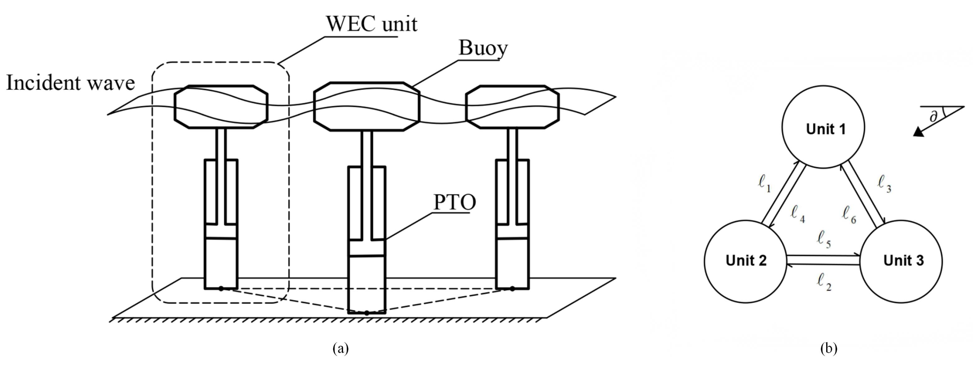
2.1. Model of WEC Unit

A point-absorber-type WEC is primarily composed of a buoy and a PTO unit, as shown in Figure 1a. The WEC array is represented as an interconnected system model in which the topology structure describes the interfering relationship between all WEC units, as shown in Figure 1b. The symbol in Figure 1b is the angle of the wave propagation direction, and 1 , , 6 denote the directed interfering relationship between each pair of the three units, Unit 1, Unit 2 and Unit 3. Buoys are used to harvest the kinetic energy of ocean waves, and PTO converts the kinetic energy of the buoy into electric energy. Meanwhile, PTO produces electric power and a damping force, which affects the motion of the buoy simultaneously excited by ocean waves.
The dynamics of a point-absorber WEC are expressed as
m f z ¨ ( t ) = F w ( t ) + F m ( t ) ,
where m f is the mass of the buoy, z ( t ) is the vertical displacement of the buoy, F w ( t ) is the hydrodynamic force, and F m ( t ) is the mechanical force.
The variables F w ( t ) and F m ( t ) satisfy
F w ( t ) = F h ( t ) + F r ( t ) + F e ( t ) , F m ( t ) = F o ( t ) + F u ( t ) ,
where F h ( t ) , F r ( t ) , F e ( t ) , F o ( t ) and F u ( t ) are the buoyancy, radiation force, excitation force, friction force of the mechanical device, and reaction force, respectively. The buoyancy F h ( t ) is
F h ( t ) = S h w ( t ) z ( t ) ,
where w ( t ) and S h are the vertical height of the incident wave and constant buoyancy coefficient, respectively. The radiation force F r ( t ) is
F r ( t ) = F D ( t ) m z ¨ ( t ) ,
where m denotes the additional mass related to the quantity of the water being moved and is used as the coefficient of the linear term of the radiation force in the case of infinite frequency. Inspired by [20], the convolution term F D ( t ) is approximated as D · w ˙ t z ˙ t , where D is a constant damping coefficient to roughly approximate the Fourier transform D ^ ( j w ) of F D ( t ) . D ^ ( j w ) can be regarded as a frequency-dependent damping coefficient.
The excitation force F e ( t ) is a non-causal force that is approximated by a fifth-order state-space representation of the relationship between the wave height and excitation force [21]. Since the influence of F o ( t ) is relatively slight, we assume F o ( t ) = 0 [22]. The proposed control algorithm calculates the reaction force F u ( t ) .
Let m = m f + m and ξ ( t ) = F h ( t ) , z ˙ ( t ) T . Then, the WEC unit model is achieved as
ξ ˙ ( t ) = A ξ ( t ) + B w w ˙ ( t ) + B F u ( t ) + F e ( t ) , y ( t ) = C ξ ( t ) , y z ( t ) = C z ξ ( t ) ,
where
A = 0 S h 1 m D m , B w = S h D m , B = 0 1 m , C = 0 1 , and C z = 1 0 .
Remark 1.
According to (5), it holds that y ( t ) = z ˙ ( t ) , and y z ( t ) = F h ( t ) .

2.2. WEC Array

2.2.1. WEC Units in Array

When the WEC units are close together, their interactions are enhanced, thus affecting the movement of the buoys more significantly. Radiation waves are the main source of interactions and therefore cannot be ignored. Considering the interaction effect, the i-th ( i = 1 , , N ) WEC unit receives the cumulative effect of the radiation wave velocity w ˙ i j generated by the other j-th ( j = 1 , , N 1 , j i ) WEC units, in addition to the effect of the incident wave velocity w ˙ i ( t ) [23]. The model of the i-th WEC unit is formulated as follows,
ξ ˙ i ( t ) = A i ξ i ( t ) + B w i w ˙ i ( t ) + j i N 1 w ˙ i j ( t ) + B i F u i ( t ) + F e i ( t ) , y i ( t ) = C i ξ i ( t ) , y z i ( t ) = C z i ξ i ( t ) ,
where ξ i ( t ) = [ F h i ( t ) , z ˙ i ( t ) ] T is the state of the i-th WEC unit, F h i ( t ) is the buoyancy of the i-th unit, z ˙ i ( t ) is the velocity of the i-th buoy. In this model, the input to the WEC unit is the total of the velocity of the incident wave and the radiated waves generated by the other WEC units.
Moreover, the array composed of N WEC units is considered as a continuous interconnected system modeled as follows:
ξ ˜ ˙ ( t ) = A c ξ ˜ ( t ) + B w c w ˜ ˙ ( t ) + B w c w ˜ ˙ ij ( t ) + B c F ˜ u ( t ) + F ˜ e ( t ) , y ˜ ( t ) = C c ξ ˜ ( t ) , y ˜ z ( t ) = C z c ξ ˜ ( t ) ,
where
ξ ˜ ( t ) = ξ 1 ξ 2 ξ N , w ˜ ˙ ( t ) = w ˙ 1 w ˙ 2 w ˙ N , w ˜ ˙ ij = j 1 N 1 w ˙ 1 j j 2 N 1 w ˙ 2 j j N N 1 w ˙ N j , F ˜ u ( t ) = F u 1 F u 2 F u N , F ˜ e ( t ) = F e 1 F e 2 F e N , y ˜ ( t ) = y 1 y 2 y N , y ˜ z ( t ) = y z 1 y z 2 y z N , A c = I N A , B w c = I N B w , B c = I N B , C c = I N C , C z c = I N C z ,
and the subscript c indicates the term of continuous system. I is an identity matrix.
Remark 2.
In this paper, a system connecting several independent WEC units with a particular network structure is called an interconnected system, where the WEC units are coupled with each other after being connected by the network. The primary distinction between the network of an interconnected system and a typical network is that the former processes dynamical edges, which can obtain system inputs based on node outputs and transmit outputs to the inputs of other nodes [24].

2.2.2. Interactions among WEC Units

According to Equation (6), w ˙ i j ( t ) indicates a variation in the vertical displacement of WEC unit i excited by the interference wave generated by WEC unit j. w ˙ i j ( t ) is associated to the locations of WEC unit i and j, and the heave motion z ˙ j ( t ) of WEC unit j. Using experimental data, and ignoring the non-linearity relationship between w ˙ i j ( t ) and z ˙ j ( t ) , this transfer function H i j ( s ) of a linear dynamic system with z ˙ j ( t ) and w ˙ i j ( t ) as input and output, respectively, can be derived by standard linear system identification techniques [23]. In addition to being an edge with dynamic properties in the network topology of the interconnected system, this linear dynamical model can be expressed simultaneously as a frequency characteristics model H i j ( j ω ) (simplified as H i j ) as follows:
w ˙ i j ( ω ) = H i j z ˙ j ( ω ) ,
H i j = j ω π | ω | 4 8 g 3 a 2 1 d i j e j ω 2 g d i j + 3 π 4 ,
where z ˙ j ( ω ) and w ˙ i j ( ω ) are defined as the Fourier transform of z ˙ j ( t ) and w ˙ i j ( t ) ; g, a and d i j are the gravity constant, the diameter of the buoy, and the distance between the i-th WEC unit and the j-th WEC unit, respectively; ω is the frequency and j is the imaginary number. For ω > 0 , the frequency characteristics model Equation (8) is equivalently formulated as [25]: 
H i j = A ( ω ) e j ϕ ( ω )
where A ( ω ) = ω 3 a 2 π 8 g 3 d i j and ϕ ( ω ) = d i j ω 2 g + π 4 . The frequency characteristics model Equation (10) as a linear system is rewritten as a state-space formula as follows:
ζ ˙ ( t ) = E ζ ( t ) + F u ( t ) , v ( t ) = H ζ ( t ) ,
where E R 5 × 5 , F R 5 × 1 , H R 1 × 5 , ζ ( t ) R 5 × 1 are the system matrix, input matrix, output matrix and state, respectively; u ( t ) and v ( t ) are the input and output of the -th interaction state-space model, respectively. Equation (11) denotes the -th ( = 1 , , 2 M , M = N ( N 1 ) 2 ) directed interaction effect between any two WEC units. This interaction effect is the weight of the corresponding edge of the interconnected system, as shown in Figure 1b.
In the WEC array, the integrated interaction model is expressed as
ζ ˜ ˙ ( t ) = E c ζ ˜ ( t ) + F c u ˜ ( t ) , v ˜ ( t ) = H c ζ ˜ ( t ) ,
where E c = I 2 M E , F c = I 2 M F , H c = I 2 M H , and
ζ ˜ ( t ) = ζ 1 ζ 2 ζ 2 M , u ˜ ( t ) = u 1 u 2 u 2 M , v ˜ ( t ) = v 1 v 2 v 2 M .

2.2.3. WEC Array System

Since a WEC array is an interconnected system, it can be represented as a graph G . The incidence matrix D of the graph G is applied to denote the interconnected system with N nodes and 2 M directed edges. The element located at the i-th row and -th column of D is defined as
D i = + 1 , node i is the head of edge , 1 , node i is the tail of edge , 0 , otherwise .
The incidence matrix D describes the connection relationship between the edges and nodes in graph G , and is used to determine the edge on which the output of the node is located and the node at which the input of the edge arrives. From the perspective of the node inputs and outputs, the incidence matrix satisfies
D = D O D I T ,
where D O and D I are the input and output matrices of the nodes, respectively, as
D O i = 1 , edge is the input of node i , 0 , otherwise . , D I i = 1 , edge is the output of node i , 0 , otherwise .
Furthermore, considering Equations (6), (11) and (13), j i N 1 w ˙ i j ( t ) in Equation (6) and u ( t ) in Equation (11) are denoted as
j i N 1 w ˙ i j ( t ) = = 1 M D O i v ( t ) , i = 1 , 2 , , N , u ( t ) = i = 1 N D I i y i ( t ) , = 1 , 2 , , 2 M .
Moreover, Equation (15) can be written in matrix form as follows
w ˜ ˙ ij ( t ) = D O v ˜ ( t ) , u ˜ ( t ) = D I y ˜ ( t ) .
For example, for the three-unit WEC array interconnected system shown in Figure 1b, the incidence matrix D is
D = 1 0 1 1 0 1 1 1 0 1 1 0 0 1 1 0 1 1 .
Considering Equation (14), the incidence matrix D is decomposed into D O and D I . According to Equations (15) and (16), we can obtain
w ˜ ˙ ij ( t ) = j 1 N 1 w ˙ 1 j ( t ) j 2 N 1 w ˙ 2 j ( t ) j 3 N 1 w ˙ 3 j ( t ) = v 1 + v 6 v 2 + v 4 v 3 + v 5 , u ˜ ( t ) = u 1 u 2 u 3 u 4 u 5 u 6 = y 2 y 3 y 1 y 1 y 2 y 3 .
By substituting Equation (16) into Equations (7) and (12), the model of a three-unit WEC array as an interconnected system is obtained. More generally, a formally uniform state-space model is achieved to express a WEC array system with N units as
ξ ˜ ˙ ( t ) ζ ˜ ˙ ( t ) = A c B w c D O H c F c D I C c E c ξ ˜ ( t ) ζ ˜ ( t ) + B w c 0 w ˜ ˙ ( t ) + B c 0 F ˜ u ( t ) + F ˜ e ( t ) , y ˜ ( t ) = C c , 0 ξ ˜ ( t ) ζ ˜ ( t ) , y ˜ z ( t ) = C z c , 0 ξ ˜ ( t ) ζ ˜ ( t ) ,
where w ˜ ˙ ( t ) = w ˜ ˙ ( t ) + w ˜ ˙ ij ( t ) .

3. MPC Algorithm Design

3.1. Control Problem Statement

Equation (19) is discretized by a zero-order hold method as
ξ ˜ ˙ ( k + 1 ) ζ ˜ ( k + 1 ) = A B w D O H F D I C E ξ ˜ ( k ) ζ ˜ ( k ) + B w 0 w ˜ ˙ ( k ) + B 0 F ˜ u ( k ) + F ˜ e ( k ) , y ˜ ( k ) = [ C , 0 ] ξ ˜ ( k ) ζ ˜ ( k ) , y ˜ z ( k ) = C z , 0 ξ ˜ ( k ) ζ ˜ ( k ) ,
where
A = e A c T , B = 0 T e A c τ d τ B c , B w = 0 T e A c τ d τ B w c , C = C c , C z = C z c , E = e E c T , F = 0 T e E c τ d τ F c , H = H c ,
w ˜ ˙ ( k ) = w ˙ 1 ( k ) w ˙ 2 ( k ) w ˙ N ( k ) , F u ˜ k = F u 1 k F u 2 k F u N k , F e ˜ k = F e 1 k F e 2 k F e N k , y ˜ k = y 1 k y 2 k y N k , y ˜ z k = y z 1 k y z 2 k y z N k .
In Equation (20), ξ ˜ k R α × N × 1 is the states set of all the WEC units at instant k, where α is the model order of each WEC unit. In addition, ζ ˜ k R β × 2 M × 1 is the states set of all interactions at time instant k, where β is the model order of each interaction. The wave excitation force and wave velocity are assumed to be predictable in this paper.
The MPC method controls the WEC array to maximize the harvesting of wave energy and convert it into electrical energy while satisfying the constraints. Since the buoy of the point-absorbing WEC is directly connected to PTO, the inner product of the buoy velocity and the corresponding reaction force is equal to the total power of the wave energy captured by the WEC array. As the velocity of the buoy is opposite to the positive direction of the reaction force, it holds that
P ( k ) = F ˜ u T ( k ) y ˜ ( k ) ,
and
max F ˜ u k k + N p T = 0 N p P k + T = min F ˜ u k k + N p T = 0 N p F u ˜ T k + T y ˜ k + T ,
where N p is the predicted time domain, and T is the time step. To ensure the convexity of the optimization problem, Equation (22) is modified as the cost function
J = T = 0 N p F ˜ u T ( k + T ) y ˜ ( k + T ) + r F ˜ u T ( k + T ) F ˜ u ( k + T ) + q y ˜ z T ( k + T ) y ˜ z ( k + T ) ,
where r and q are two artificially determined weighting factors. The first part of the cost function Equation (23) is the wave energy harvesting power in Equation (22). The second part of Equation (23) represents a soft constraint on the control force, primarily to guarantee that the solution of the MPC is to solve a convex optimization problem and the control force is within the PTO’s operating range. The third part represents the penalty term of the relative displacement of the buoy and the wave surface, ensuring the PTO operates within an effective operating range. To guarantee the safe operation of the WEC array and reduce the loss and maintenance cost, it is necessary to restrict the amplitude of the reaction force. Moreover, the buoy needs to be constrained to keep the proportional displacement between the midpoint of the buoy and the wave surface within a safe range. These constraints are formulated as follows,
F u k + T F u , m a x , for T = 0 , 1 , , N p , y z k + T y z , m a x , for T = 0 , 1 , , N p ,
where F u , m a x and y z , m a x are the maximum amplitude of the control force and buoyancy, respectively.
The MPC aims to solve the optimal control input sequence that minimizes the cost function Equation (23) in the prediction time domain N p , under the premise that the constraint Equation (24) is satisfied.
Remark 3.
The weighting factors r and q in Equation (23) are specified as two specific values independently to ensure that the MPC is a convex optimization problem.

3.2. Prediction Model

The cost function Equation (23) can be expressed in matrix form as
J = U ˜ k k + N p T Y ˜ k k + N p + U ˜ k k + N p T R U ˜ k k + N p + Y ˜ z k k + N p T Q Y ˜ z k k + N p ,
where R = r × I N × N P + 1 , Q = q × I N × N P + 1 ,
U ˜ k k + N p = F ˜ u ( k ) F ˜ u ( k + 1 ) F ˜ u k + N p , Y ˜ k k + N p = y ˜ ( k ) y ˜ ( k + 1 ) y ˜ k + N p , Y ˜ z k k + N p = y ˜ z ( k ) y ˜ z ( k + 1 ) y ˜ z k + N p ,
and I is a unit diagonal matrix.
In the cost function, it is necessary to know the buoy velocity and buoyancy of each unit in the predicted time domain. By the discrete model of the interconnected system, we derive a prediction model from k to k + N p as follows:
Y ˜ k k + N p = Λ X k + Φ u U ˜ k k + N p + F ˜ e k k + N p + Φ w W ˜ ˙ k k + N p , Y ˜ z k k + N p = Λ z X ( k ) + Φ u z U ˜ k k + N p + F ˜ e k k + N p + Φ w z W ˜ ˙ k k + N p ,
where
X ( k ) = ξ ˜ ( k ) ζ ˜ ( k ) , F ˜ e k k + N p = F ˜ e ( k ) F ˜ e ( k + 1 ) F ˜ e k + N p , W ˜ ˙ k k + N p = w ˜ ˙ ( k ) w ˜ ˙ ( k + 1 ) w ˜ ˙ k + N p , Λ = C C A C A 2 C A N p ,
Φ u = 0 C B u 0 C A B u C B u 0 C A N p 1 B u C A N p 2 B u C B u 0 ,
Φ w = 0 C B w 0 C A B w C B w 0 C A N p 1 B w C A N p 2 B w C B w 0 ,
Λ R N × N p + 1 × ( α N + 2 β M ) , Φ u R N × N p + 1 × N × N p + 1 ,
Φ w R N × N p + 1 × N × N p + 1 ,
with
A = A B w D i H F D i C E , B u = B 0 , B w = B w 0 , C = [ C , 0 ] , C z = [ C z , 0 ] .
Similarly, Λ z , Φ u z and Φ w z need to replace C in the corresponding matrix element by C z . Using prediction models Equation (24) to represent their constraints in the predicted time domain achieves
U ˜ k k + N p U max , Λ z x ( k ) + Φ u z U ˜ k k + N p + F ˜ e k k + N p + Φ w z W ˜ ˙ k k + N p Y z , max ,
with
U max = F u , max F u , max F u , max R N × N p × 1 , Y z , max = y z , max y z , max y z , max R N × N p × 1 .

3.3. Quadratic Programming Problem

We need to solve the optimal reaction force sequence so that the cost function J can obtain the minimum value as
U ˜ k * k + N p = arg min U ˜ k k + N p J .
Equation (25) is reorganized into a general form to utilize the standard QP solver.
Substituting the prediction model Equation (26) into the cost function Equation (25), and ignoring terms unrelated to U ˜ k k + N p , leads to
J = 1 2 U ˜ k k + N p T H U ˜ k k + N p + F T U ˜ k k + N p ,
where
H = Φ u + Φ u T + 2 R + 2 Φ u z T Q Φ u z , F = Λ + 2 Φ u z T Q Λ z X ( k ) + Φ w + 2 Φ u z T Q Φ w z W ˜ ˙ k k + N p + Φ u + 2 Φ u z T Q Φ u z F ˜ e k k + N p .
The constraints Equation (27) are reorganized into
S U ˜ k k + N p b u ,
where S = I I Φ u z Φ u z , and b u = U max U max Y z , max Λ x z x ( k ) Φ w z W ˜ ˙ k k + N p Φ u z F ˜ e k k + N p Y z , max + Λ x z x ( k ) + Φ w z W ˜ ˙ k k + N p + Φ u z F ˜ e k k + N p .
Finally, the general form of the QP problem is summarized as
U ˜ * = arg min U 0 k 1 2 U ˜ k k + N p T H U ˜ k k + N p + F T U ˜ k k + N p , S . t . S U ˜ k k + N p b u .
In each control horizon, the first term U ˜ k k + 1 in the sequence of optimal control forces U ˜ k * k + N p is adopted as the optimal control force at time k.

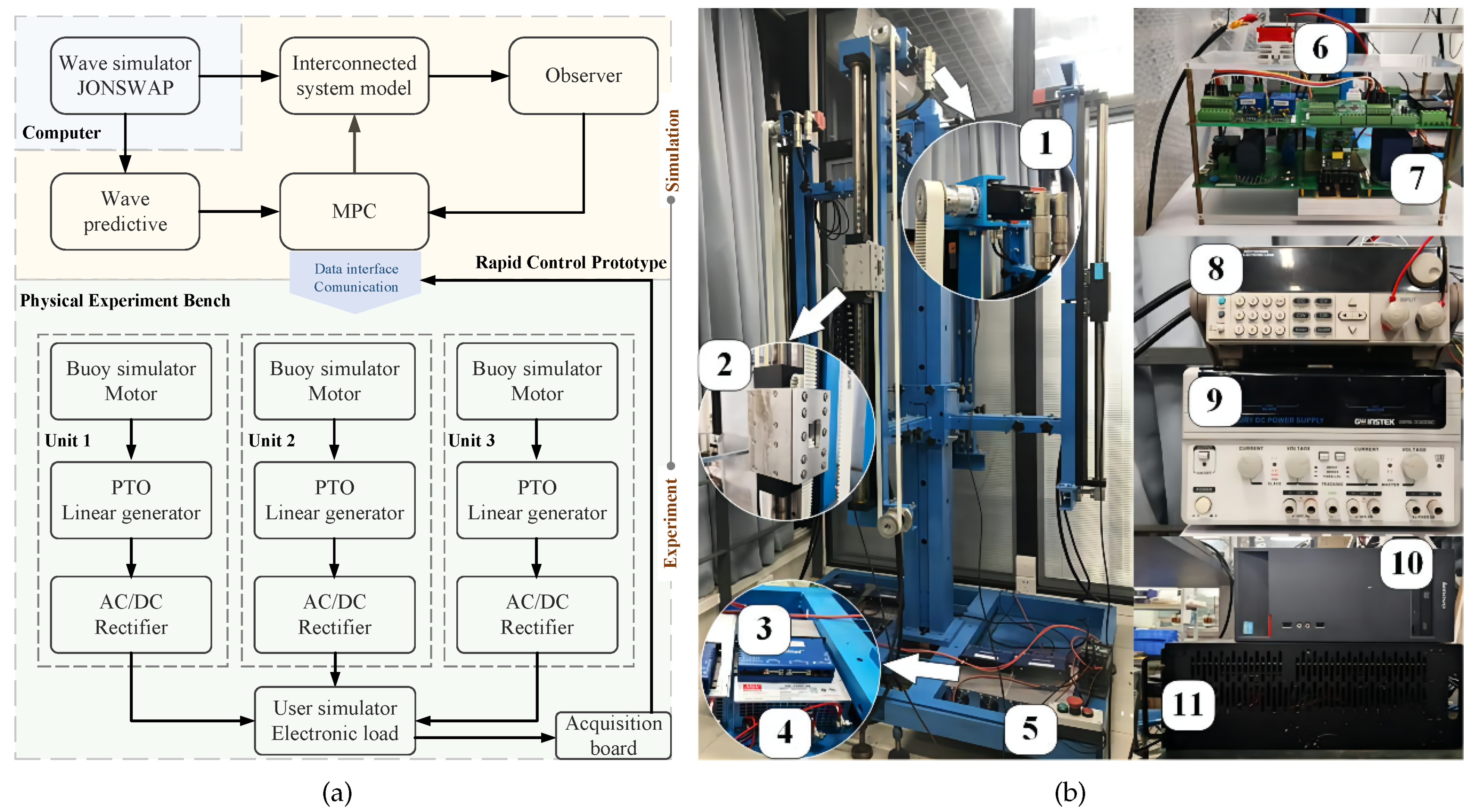
4. Experimental Results and Discussion

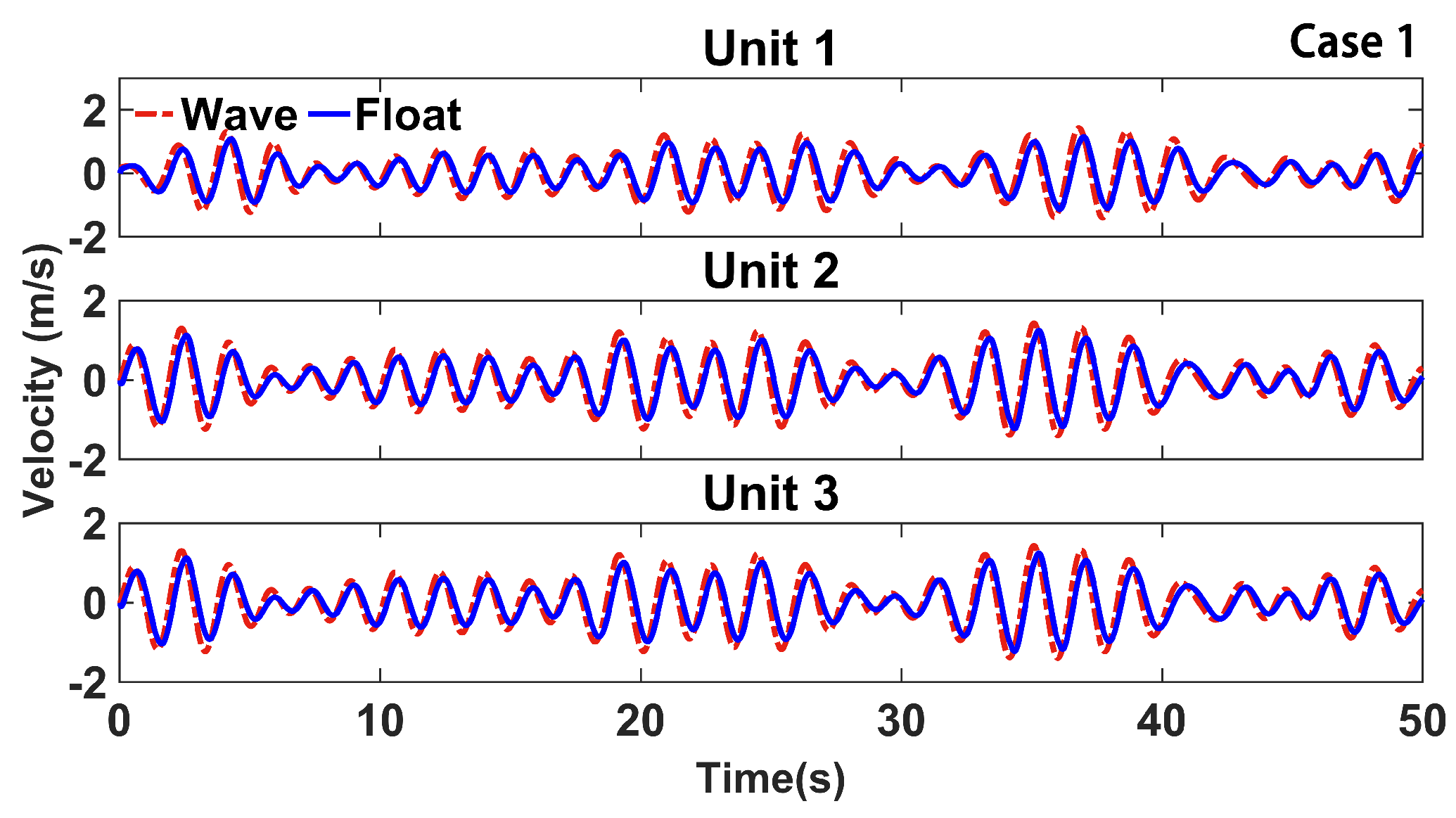
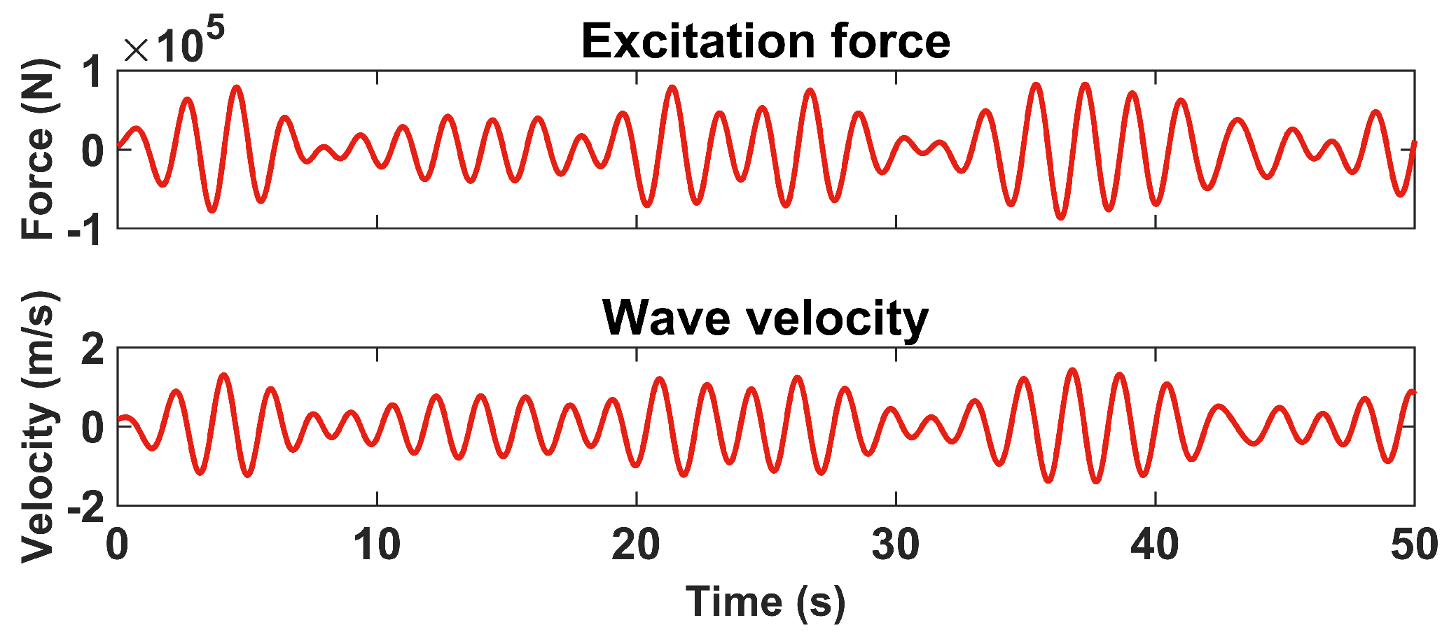
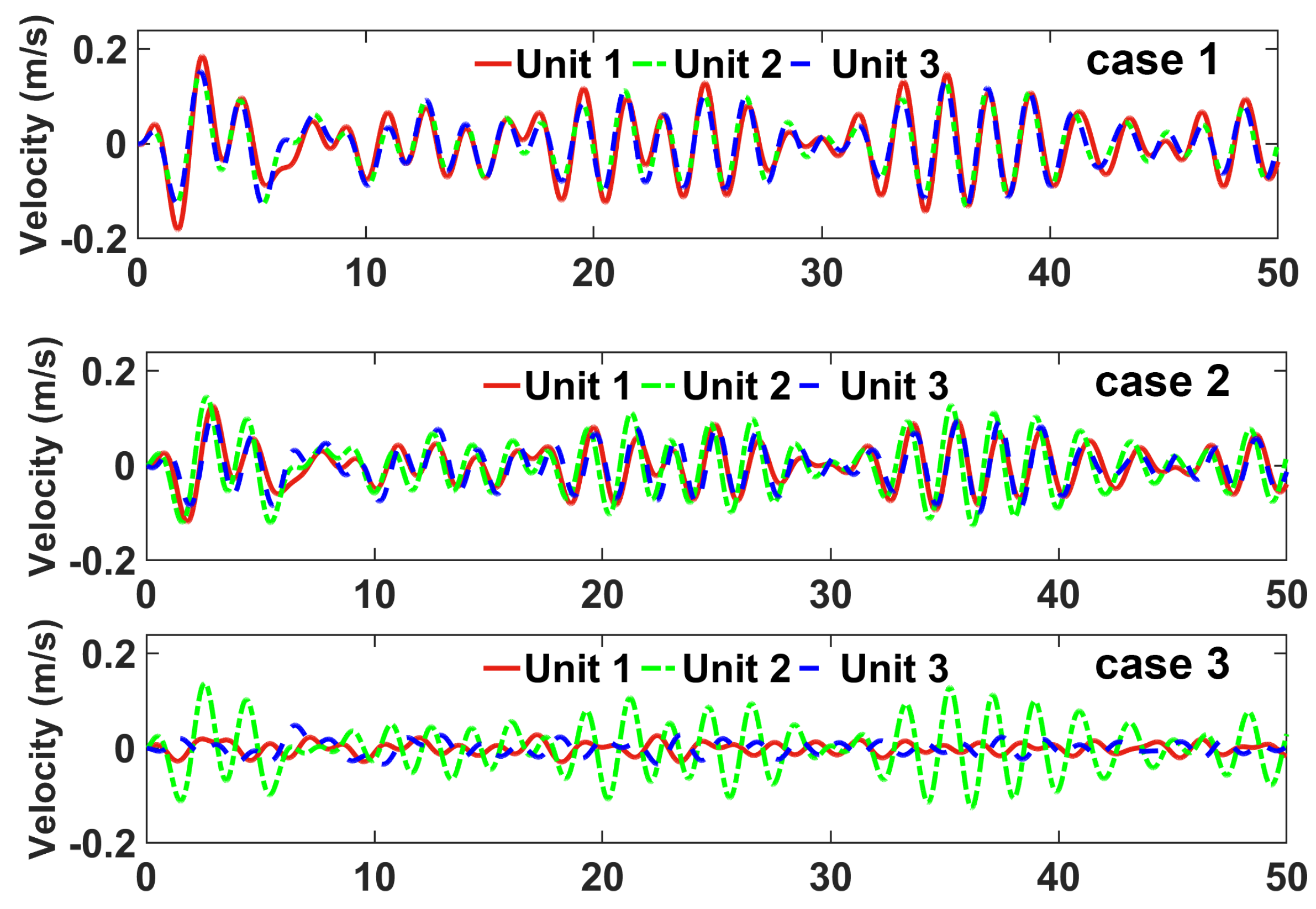
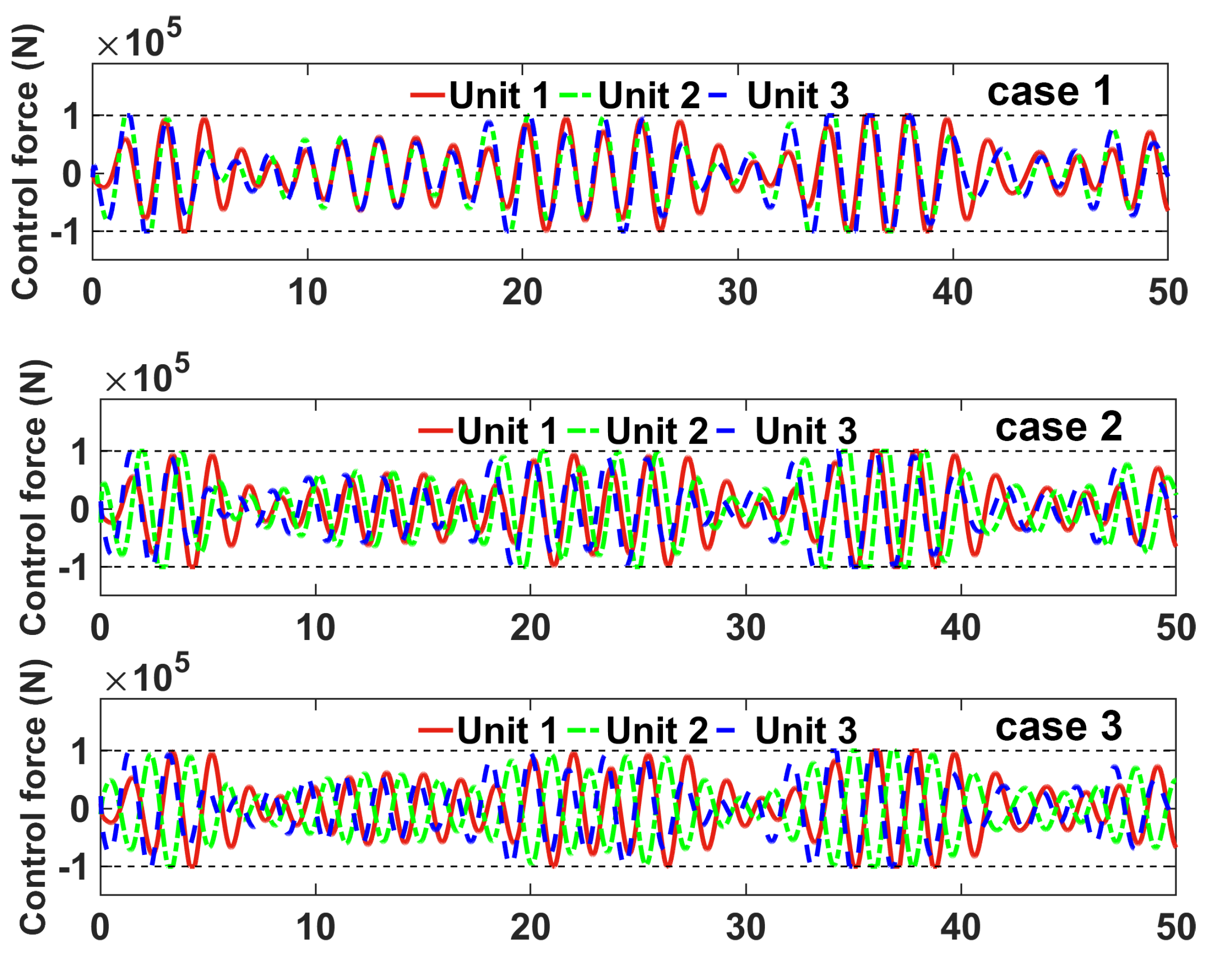
4.1. Simulation of Wave Energy Harvesting

We designed a semi-physical hardware-in-the-loop (HIL) experiment to simulate the wave energy capture more realistically than the digital simulation, and to reduce the high cost and complexity of the real ocean or large pool environment. The semi-physical experimental platform consisted of a front-end part and a back-end part as shown in Figure 2a. The front-end part comprised a desktop computer running MATLAB ® and an RT-LAB simulator (a rapid control prototyping (RCP) platform from OPAL-RT Technologies Canada), as shown in the upper part of Figure 2a. The front-end part was mainly dedicated to simulating realistic sea conditions to implement a fully digital simulation of the WEC array to validate the established interconnected system model and the MPC control strategy mapped to the back-end part for the physical experiment bench operation.
The back-end part was a physical experiment bench as shown in the lower part of Figure 2a,b. The rotating motor was controlled by a commercial drive (Copley Controls ADP-090-36) and was used to imitate the rippling motion of the WEC buoys in the array under the effect of wave force. As the PTO device of the WEC, the linear generator (see Table 1 for the specific parameters) was dragged by a belt to convert the motion of the simulated buoy into an AC power output. The AC power generated by three PTO devices was converted to DC power using an AC-DC converter and rectifier (modules 6 and 7 in Figure 2b) developed in our laboratory and fed to the DC bus and electronic loads.
The purpose of constructing the above experimental system was to perform the following procedures:
(i)
Verifying the correctness of the interconnected model and the control performance of the proposed MPC algorithm;
(ii)
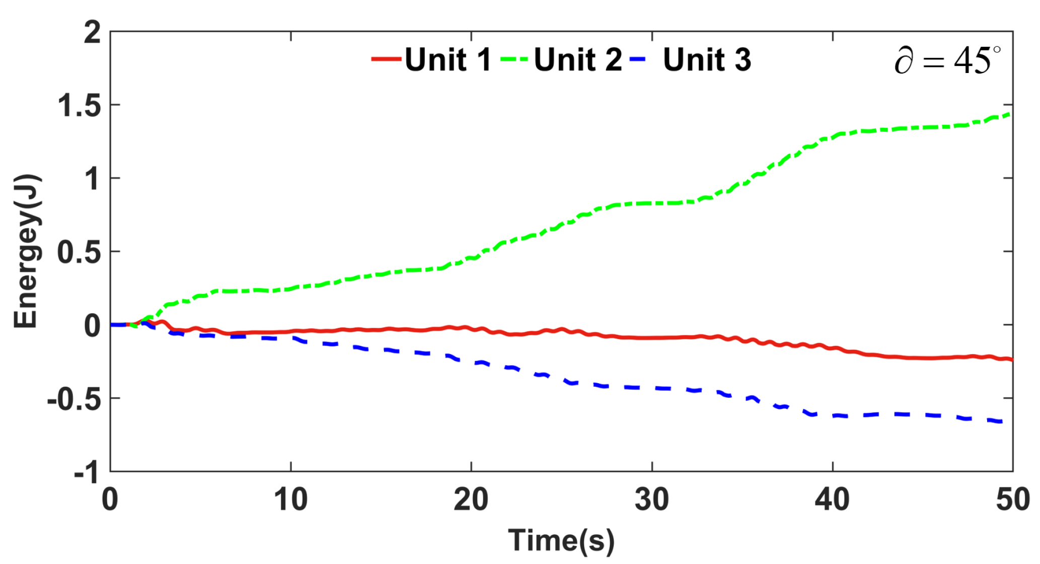
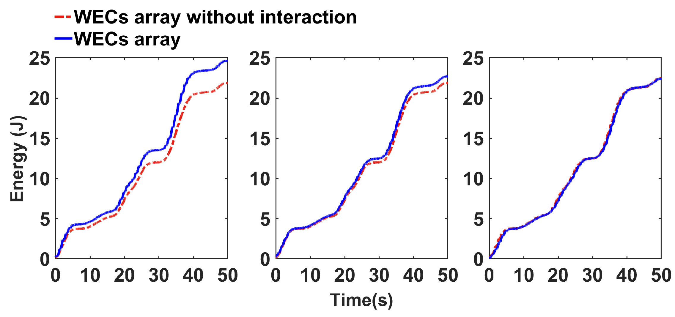
Comparing the difference in the motion characteristics affected by the interaction and the wave energy harvesting efficiency between the interconnected model and the isolated model of the WEC array, and exploring how to affect the wave energy harvesting efficiency by change in the incident wave propagation direction in the WEC interconnected system.

4.2. Simulation Parameter Setting

We built a three-unit WEC array in the front end with reference to the PB3 device described in [26,27] developed by Ocean Power Technologies Inc. All the parameters are shown in Table 2. The three WEC units were arranged in an equilateral triangle with a distance of 25 m from each other.
The JONSWAP function generated the incident wave [28]; the wave significant height was 2 m, and the peak period was 3 s. The wave velocity and the corresponding wave excitation force F e are shown in Figure 3. To investigate the effect that the angle of wave propagation direction waves had on the WEC array, three sets of experiments with different wave propagation directions = 30 , 45 , 60 were set up.

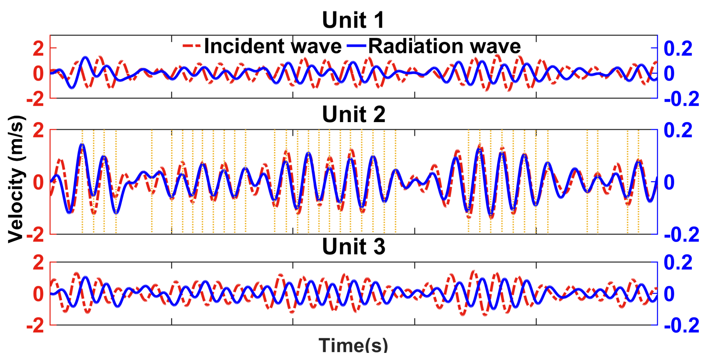
4.3. Results and Discussion

The prediction horizon and the control horizon were both 10 s , the sampling time was 0.02 s , and the simulation time was 50 s . The weight value r was set to 2.5 × 10 6 to ensure that the Hermitian matrix was a positive definite matrix, and Q was also set to 2.5 × 10 6 . When the radius of the buoy was 5 × a m and the distance d i j was 25 m , the matrices of the state-space representation of the edge model were
E = 1.3192 2.6404 1.8147 1.3222 0.2090 1 1 1 1 , F = 1 0 0 0 0 T , and H = 0.1470 0.1931 0.1043 0.0100 0.0053 .
Figure 4 shows the velocity of each unit’s radiation wave in the three layout cases. In particular, when = 30 , Units 2 and 3 were affected by the same interference. This was because of the symmetrical structure of the equilateral triangle, and the propagation direction of the incident wave overlapping the symmetric axis, so that the waveform of the incident wave received by Units 2 and 3 was synchronized, and the identical edge model caused the same interference. Figure 5 shows that, under the control of the MPC algorithm, the control force of each WEC unit was limited to a range of ± 1 × 10 5 N, which satisfies the input constraint in Table 1.
In Figure 6, the waveform of each buoy velocity is almost the same as that of the corresponding incident wave velocity, and resonance is almost realized between the buoy motion and the wave motion. Due to the existence of other terms in the cost function, the execution delay, and the limitation of the control force and displacement, the resonance between the buoy and the incident wave is not fully realized. However, the wave energy capture efficiency is optimized by the control of the MPC algorithm.
To show the impact of interactions in the interconnected system, three units of isolated systems were set up as baseline cases. The isolated system had no interaction among the three WEC units. Thus, the radiation waves caused by the oscillating motion of units did not affect the neighborhood units. In the mathematical model Equation (20), the induction matrix D is an all-0 matrix. Because the interaction exists in the WEC array, the buoy’s motion velocity is different between the interconnected and isolated systems without interaction. Furthermore, to adapt to the existence of the interaction, the MPC algorithm solves the optimal reaction force to make the units coordinate with each other to achieve the global optimal efficiency.
Figure 7 shows the variation in the total power generated by the corresponding three WEC units between the interconnected and the isolated system when the wave incidence angle = 45 . Each curve in Figure 7 illustrates the difference in wave energy captured by a unit, taking into account the impact of interfering waves between units compared with those not taking into account interfering waves. The energy error curves for the three units in Figure 7 highlight the various effects of interactions within the array on the energy harvesting of each unit. Figure 8 shows the waveform of the radiation wave and the incident wave when the incident wave angle = 45 . Note that in Figure 7, Unit 2 of the interconnected system harvests more wave energy than Unit 2 of the isolated system. In Figure 8, the waveforms of the incident wave received by Unit 2 are nearly the same as those of the radiation wave generated by the other units. The wave energy harvested by Units 1 and 3 of the interconnected system is not as high as the corresponding unit in the isolated system, and the waveforms of the incident wave and the radiation wave are significantly asynchronous.
When the waveform of the radiation wave received by the WEC unit is close to that of the incident wave, the unit can generate more energy. When their phase error is close to zero, so that the radiation wave synchronizes with the incident wave, just as when the buoy motion synchronizes with the wave motion, the efficiency of the wave energy captured by the WEC is optimized. At this time, the radiation wave also enables maximum optimization of the wave energy captured by the corresponding unit of the interconnected system.
To show the influence of the interaction in different cases, we define the index ϱ as
ϱ = P array , i j = 1 N P isolate , i j ,
where P array , i and P isolate , i j are the power of the WEC array as an interconnected system and the power of each isolated unit at t = i , respectively.
In the three cases, the interaction of the interconnected system had a positive or negative effect at different instances within 50 s. The interaction in the first and second cases had more positive than negative effects, and ϱ > 1 was satisfied, respectively, 62.72 % and 52.08 % of the total time. In the third case, the negative effect was more than the positive effect, and ϱ > 1 was satisfied only 29.08 % of the total time.
The results in Figure 9 show that in the first and second cases, the interconnected system controlled by the MPC algorithm had higher wave energy harvesting efficiency than the isolated system. In the third case, the interconnected system harvested less wave energy than the isolated system. In addition, when the incident waves had different propagation directions, the increase in the wave energy harvesting efficiency of the WEC interconnected system changed accordingly.

5. Conclusions

In this paper, we proposed an interconnected system model of a WEC array which graphically integrates a WEC unit model and an interference model. The proposed model with wave interference dynamics describes the WEC array system more accurately. Each part of the interconnected system model has a well-defined structure that can better reflect uniformity when the array configuration changes. The interconnected model accurately describes the wave energy harvesting process under the influence of wave interference. The MPC algorithm based on the interconnected system model is applied to enable the WEC array to achieve optimal global performance of wave energy capture control, subject to several constraints. Through experimental tests, it was found that the phase error between the radiation and incident waves significantly affected the wave energy capture efficiency, and the wave energy capture efficiency was effectively improved as the error decreased. The experimental results show that the MPC with the interconnected system model had a higher wave energy capture efficiency compared with the isolated system model. However, the performance of the MPC relies on accurate and sufficient information on wave excitation forecasts. Future research will concentrate on more realistic hydrodynamics of the buoys and their coupling in the ocean environment, as well as inaccurate or insufficient wave excitation forecasts. Strengthening the robustness and adaptability of the MPC controller by combining intelligent control techniques is another promising direction.

Author Contributions

All authors contributed to the study conception and design. Administrative support and provision of study materials were provided by B.Z., X.B. and A.K.; collection and assembly of data were undertaken by H.Z., S.Y.; data analysis and interpretation were performed by B.Z., S.C., X.B. and A.K. All authors have read and agreed to the published version of the manuscript.

Funding

This work is supported in part by the National Natural Science Foundation of China under Grants 62173234 and 62003217.

Institutional Review Board Statement

Not applicable.

Informed Consent Statement

Not applicable.

Data Availability Statement

All data generated or analysed during the study of this manuscript are included in the article.

Conflicts of Interest

With respect to the content of this paper, all the authors have no conflict of interest to declare.

References

  1. O’Sullivan, A.; Sheng, W.; Lightbody, G. An analysis of the potential benefits of centralised predictive control for optimal electrical power generation from wave energy arrays. IEEE Trans. Sustain. Energy 2018, 9, 1761–1771. [Google Scholar] [CrossRef]
  2. Babarit, A. On the park effect in arrays of oscillating wave energy converters. Renew. Energy 2013, 58, 68–78. [Google Scholar] [CrossRef]
  3. Kagemoto, H.; Yue, D.K. Interactions among multiple three–dimensional bodies in water waves: An exact algebraic method. J. Fluid Mech. 1986, 166, 189–209. [Google Scholar] [CrossRef]
  4. Babarit, A.; Borgarino, B.; Ferrant, P.; Clément, A.H. Assessment of the influence of the distance between two wave energy converters on energy production. IET Renew. Power Gener. 2009, 4, 592–601. [Google Scholar] [CrossRef]
  5. Borgarino, B.; Babarit, A.; Ferrant, P. Impact of wave interactions effects on energy absorption in large arrays of wave energy converters. Ocean Eng. 2012, 41, 79–88. [Google Scholar] [CrossRef]
  6. Devolder, B.; Stratigaki, V.; Troch, P.A.; Rauwoens, P. CFD simulations of floating point absorber wave energy converter arrays subjected to regular waves. Energies 2018, 11, 641. [Google Scholar] [CrossRef]
  7. Chen, W.; Gao, F.; Meng, X.; Fu, J. Design of the wave energy converter array to achieve constructive effects. Ocean Eng. 2016, 124, 13–20. [Google Scholar] [CrossRef]
  8. Fang, H.; Feng, Y.; Li, G. Optimization of wave energy converter arrays by an improved differential evolution algorithm. Energies 2018, 11, 3522. [Google Scholar] [CrossRef]
  9. Sharp, C.; DuPont, B. Wave energy converter array optimization: A genetic algorithm approach and minimum separation distance study. Ocean. Eng. 2018, 163, 148–156. [Google Scholar] [CrossRef]
  10. Previsic, M.; Karthikeyan, A.; Scruggs, J.T. A comparative study of model predictive control and optimal causal control for heaving point absorbers. J. Mar. Sci. Eng. 2021, 9, 805. [Google Scholar] [CrossRef]
  11. Faedo, N.; Olaya, S.; Ringwood, J.V. Optimal control, MPC and MPC–like algorithms for wave energy systems: An overview. IFAC J. Syst. Control 2017, 1, 37–56. [Google Scholar] [CrossRef]
  12. Haider, A.S.; Brekken, T.K.; Mccall, A.K. Real-Time nonlinear model predictive controller for multiple degrees of freedom wave energy converters with non–ideal power take-off. J. Mar. Sci. Eng. 2021, 9, 890. [Google Scholar] [CrossRef]
  13. Jia, Y.; Meng, K.; Dong, L.; Liu, T.; Sun, C.; Dong, Z.Y. Economic model predictive control of a point absorber wave energy converter. IEEE Trans. Sustain. Energy 2021, 12, 578–586. [Google Scholar] [CrossRef]
  14. Montoya, D.G.; Tedeschi, E.; Castellini, L.; Martins, T.D. Passive model predictive control on a two–body self–referenced point absorber wave energy converter. Energies 2021, 14, 1731. [Google Scholar] [CrossRef]
  15. Haider, A.S.; Brekken, T.K.; Mccall, A.K. Application of real-time nonlinear model predictive control for wave energy conversion. IET Renew. Power Gener. 2021, 15, 3331–3340. [Google Scholar] [CrossRef]
  16. Richter, M.; Magaña, M.E.; Sawodny, O.; Brekken, T.K. Nonlinear model predictive control of a point absorber wave energy converter. IEEE Trans. Sustain. Energy 2013, 4, 118–126. [Google Scholar] [CrossRef]
  17. Oetinger, D.; Magaña, M.E.; Sawodny, O. Decentralized model predictive control for wave energy converter arrays. IEEE Trans. Sustain. Energy 2014, 5, 1099–1107. [Google Scholar] [CrossRef]
  18. Oetinger, D.; Magaña, M.E.; Sawodny, O. Centralised model predictive controller design for wave energy converter arrays. IET Renew. Power Gener. 2015, 9, 142–153. [Google Scholar] [CrossRef]
  19. Vicente, P.C.; Falcão, A.F.; Gato, L.M.; Justino, P.A. Dynamics of arrays of floating point-absorber wave energy converters with inter-body and bottom slack-mooring connections. Appl. Ocean Res. 2009, 31, 267–281. [Google Scholar] [CrossRef]
  20. Li, G.; Belmont, M. Model predictive control of sea wave energy converters—Part I: A convex approach for the case of a single device. Renew. Energy 2014, 69, 453–463. [Google Scholar] [CrossRef]
  21. Yu, Z.; Falnes, J. State-Space modelling of a vertical cylinder in heave. Appl. Ocean Res. 1995, 17, 265–275. [Google Scholar] [CrossRef]
  22. Jama, M.A.; Wahyudie, A.; Noura, H. Robust predictive control for heaving wave energy converters. Control. Eng. Pract. 2018, 77, 138–149. [Google Scholar] [CrossRef]
  23. Li, G.; Belmont, M. Model predictive control of sea wave energy converters—Part II: The case of an array of devices. Renew. Energy 2014, 68, 540–549. [Google Scholar] [CrossRef]
  24. Coogan, S.D.; Arcak, M. A dissipativity approach to safety verification for interconnected systems. IEEE Trans. Autom. Control 2015, 60, 1722–1727. [Google Scholar] [CrossRef]
  25. Falnes, J. Radiation impedance matrix and optimum power absorption for interacting oscillators in surface waves. Appl. Ocean Res. 1980, 2, 75–80. [Google Scholar] [CrossRef]
  26. Product Specifications for the pb3. Available online: https://oceanpowertechnologies.com/product/ (accessed on 1 March 2021).
  27. Viet, N.V.; Carpinteri, A.; Wang, Q. A novel heaving ocean wave energy harvester with a frequency tuning capability. Arab. J. Sci. Eng. 2019, 44, 5711–5722. [Google Scholar] [CrossRef]
  28. Aranuvachapun, S. Parameters of JONSWAP spectral model for surface gravity waves—I. Monte Carlo simulation study. Ocean Eng. 1987, 14, 89–100. [Google Scholar] [CrossRef]
Figure 1. Point absorption WEC array: (a) the structure of the point-absorber-type WEC; (b) the interfering relationship between three units.
Jmse 10 01033 g001
Figure 2. Experimental bench: (a) Framework; (b) Hardware: 1. Rotating motor; 2. Linear motor; 3. Driver; 4. DC power; 5. Switch; 6. Rectifier; 7. Acquisition board; 8. Electronic load; 9. DC power; 10. Computer; 11. RT-LAB.
Jmse 10 01033 g002
Figure 3. Excitation force and wave velocity.
Jmse 10 01033 g003
Figure 4. Interaction of radiation wave velocities received by each unit.
Jmse 10 01033 g004
Figure 5. Reaction force controlled by the MPC algorithm.
Jmse 10 01033 g005
Figure 6. Buoy velocity and incident wave velocity.
Jmse 10 01033 g006
Figure 7. Variation in the wave energy harvested by each WEC unit between the interconnected and isolated systems.
Jmse 10 01033 g007
Figure 8. Wave velocity of the interacting radiation wave and the incident wave.
Jmse 10 01033 g008
Figure 9. Electrical energy generated by the WEC array and WEC array without interaction.
Jmse 10 01033 g009
Table 1. Specifications for wave energy linear generators.
Electrical ParametersValueMechanical ParametersValue
Rated power (W)50Mover stroke (cm)70
Rated current (A)20Mover speed (m/s) 3.5 m
Rated voltage (V)20Mover length (cm)18
Conversion efficiency 85 % Mover weight (kg) 1.65
Table 2. Simulation parameters.
DescriptionNotationValue
Diametera 2.65 m
Heighth 3.5 m
DampingD 2 × 10 5 Nm/s
Buoy massm8300 kg
Added mass m 6100 kg
Stiffness S h 2.21 × 10 5 N/m
Density of sea water ρ 1020 kg/m 3
Gravityg 9.81 m/s 2
Maximum heave motion y z , max 1.75 m
Maximum input magnitude F u , max 1 × 10 5 N
Publisher’s Note: MDPI stays neutral with regard to jurisdictional claims in published maps and institutional affiliations.

