
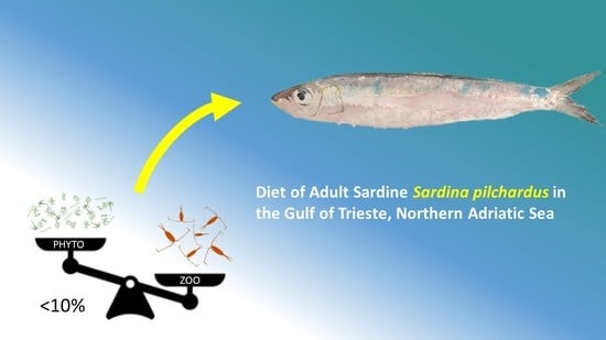
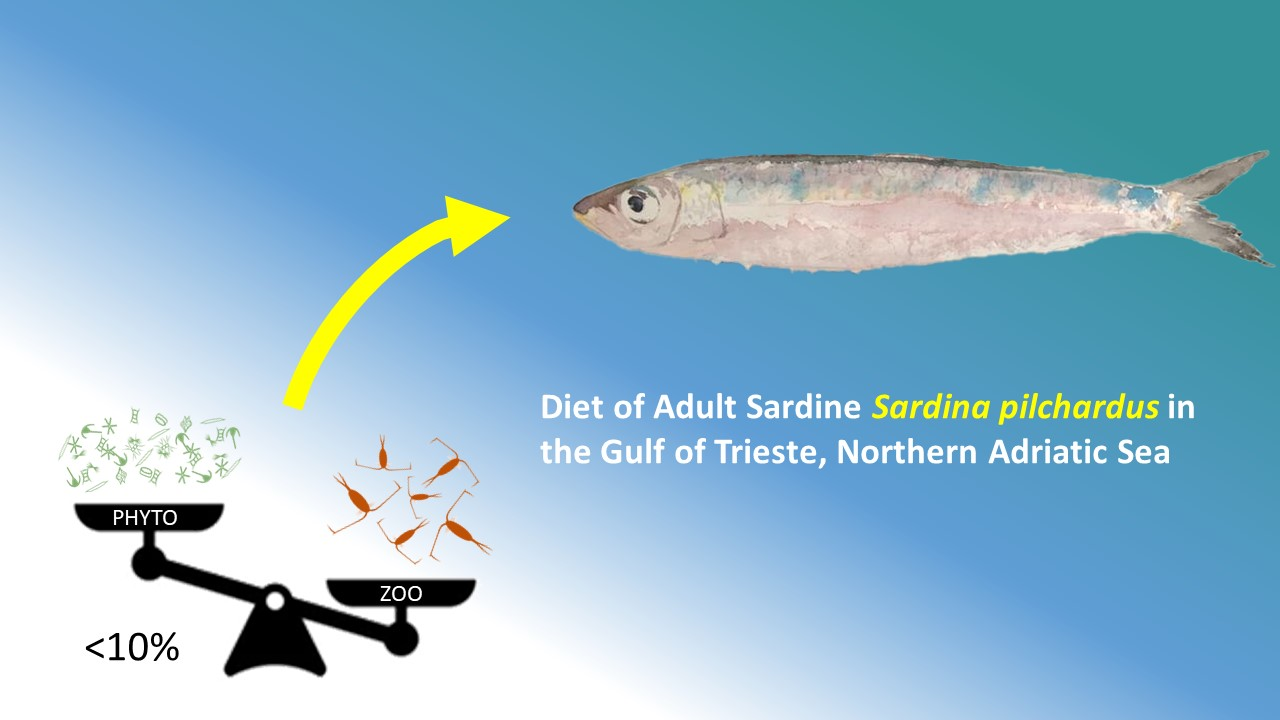
Diet of Adult Sardine Sardina pilchardus in the Gulf of Trieste, Northern Adriatic Sea


Abstract
1. Introduction
2. Materials and Methods
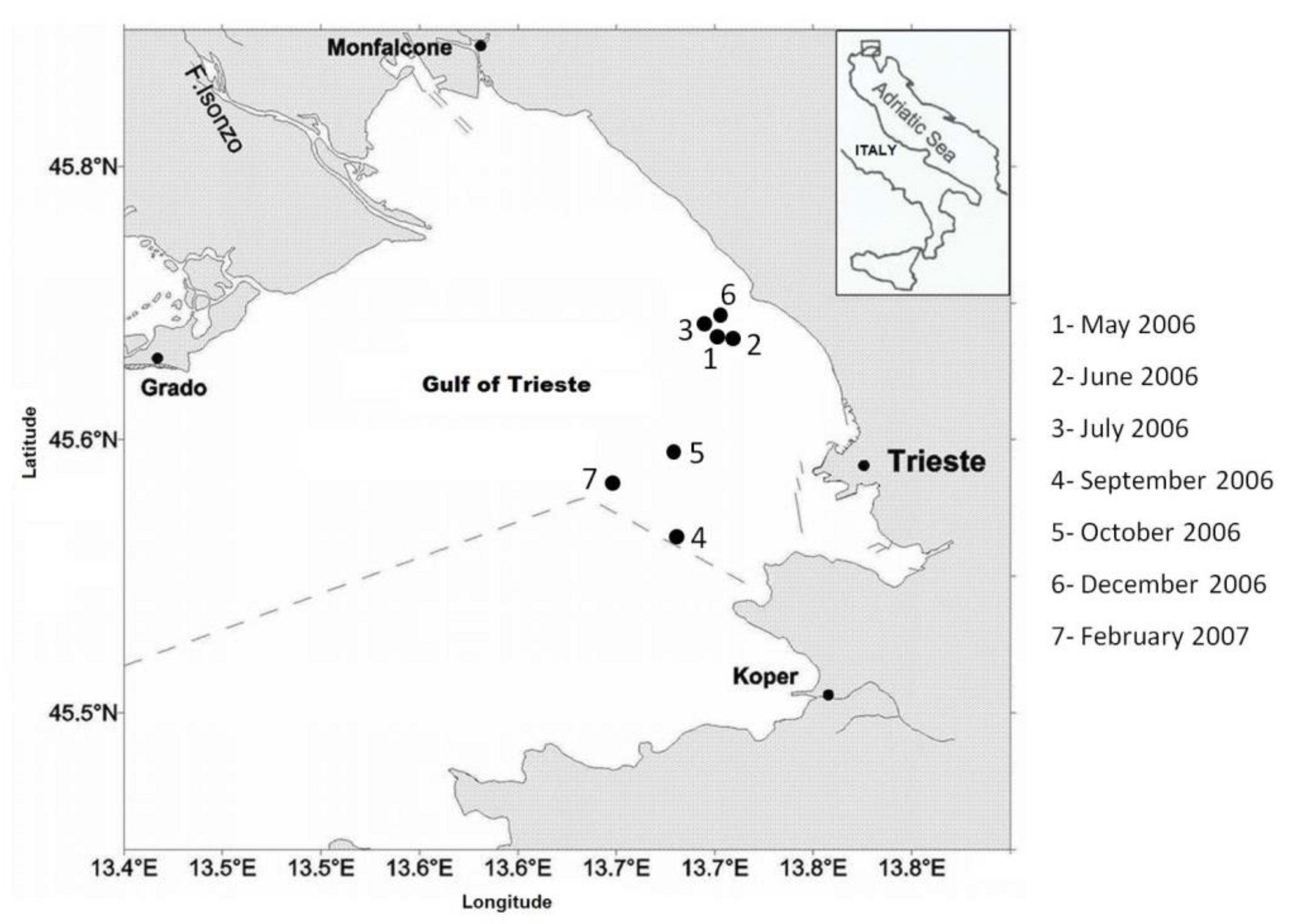
2.1. Study Area
2.2. Field Sampling
2.3. Diel Feeding Cycle
2.4. Diet Composition and Dietary Carbon
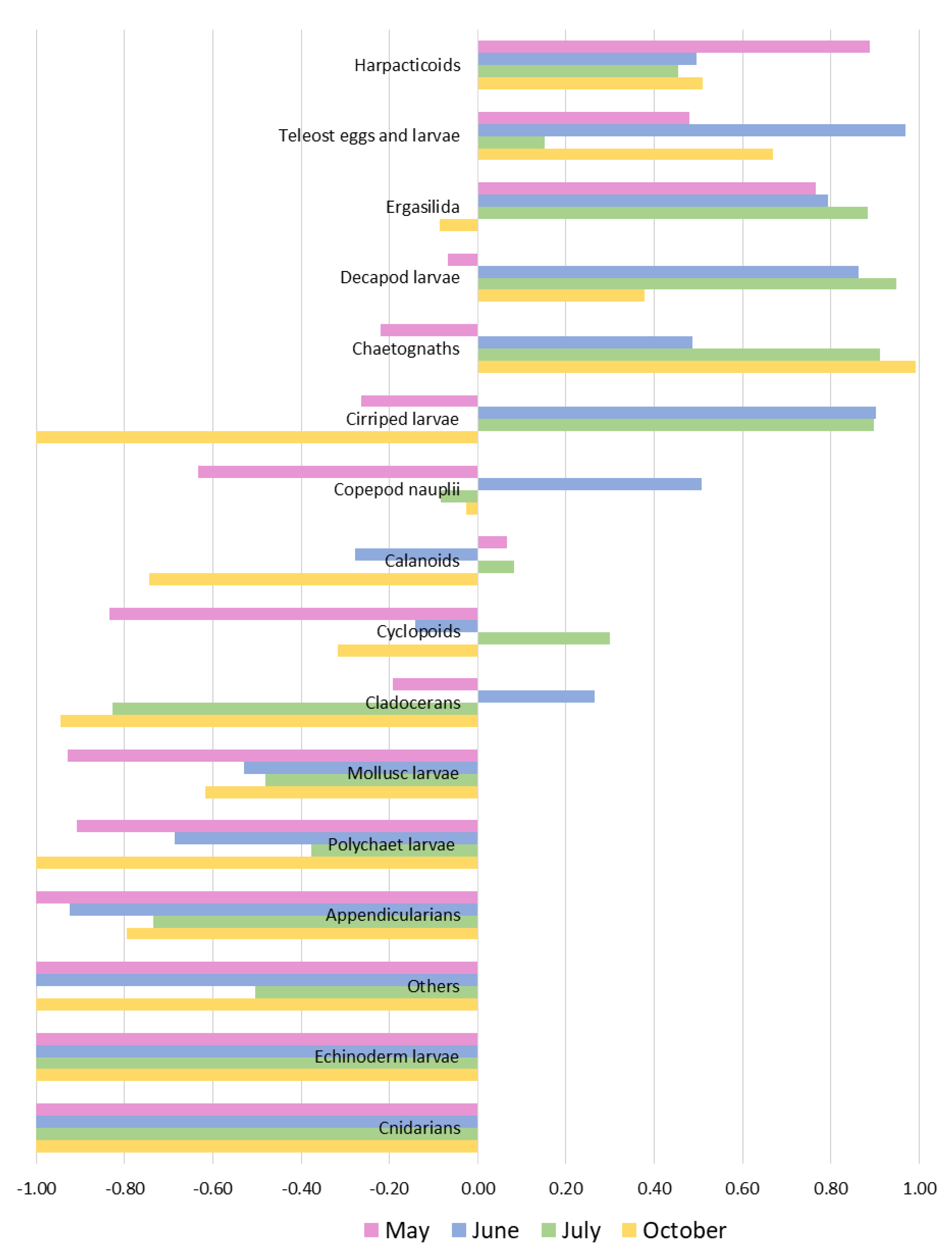
2.5. Feeding Selectivity
3. Results
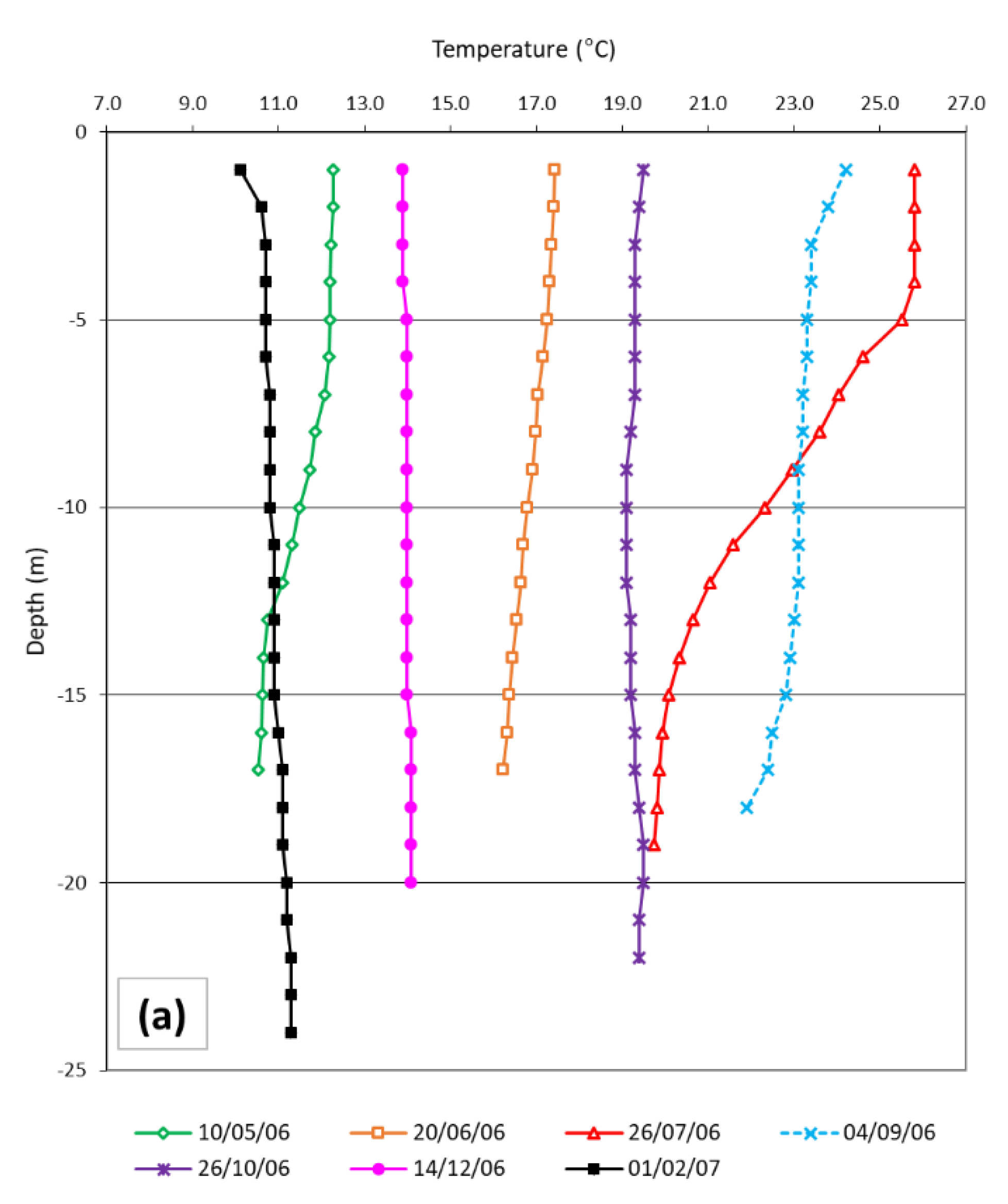
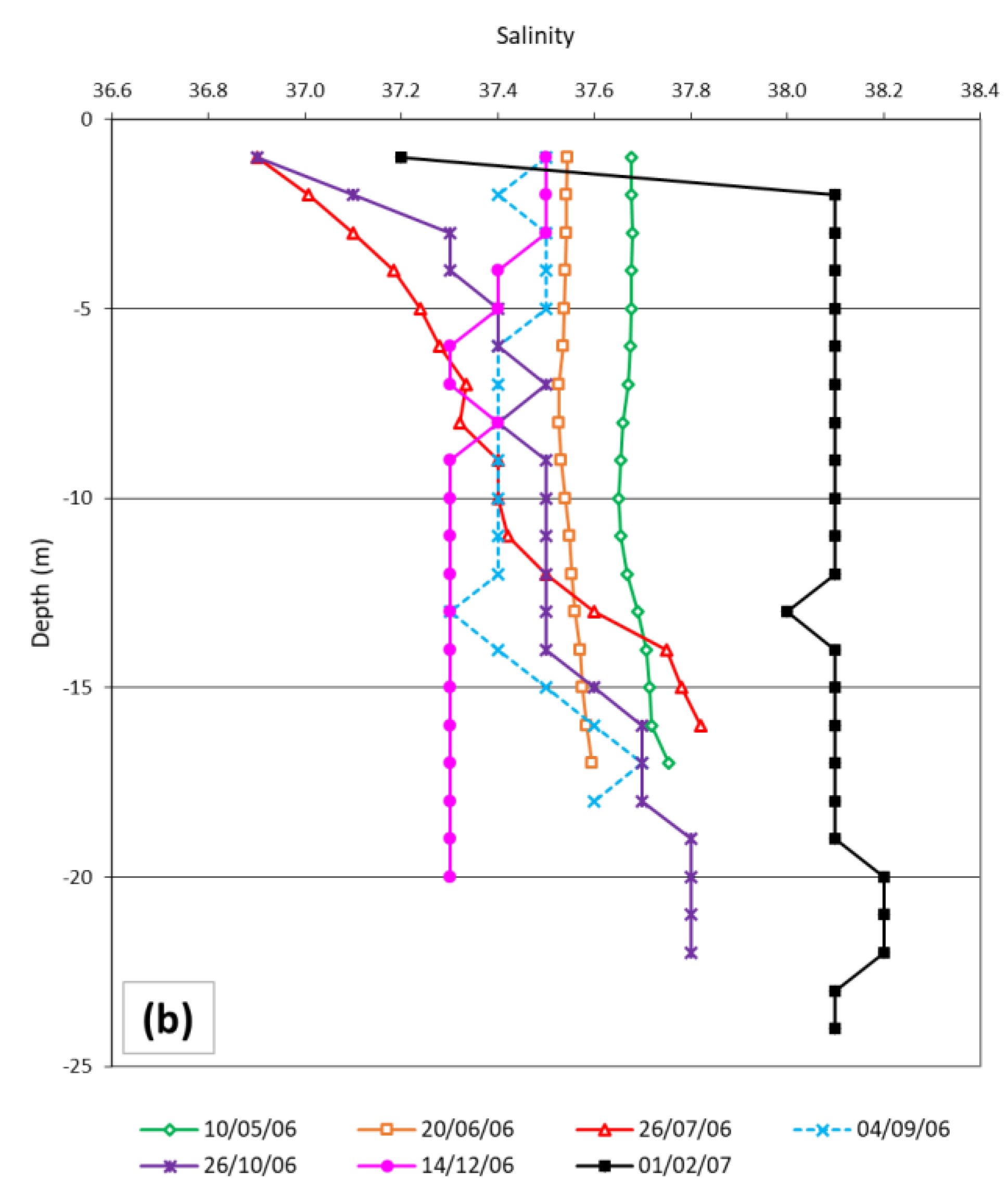
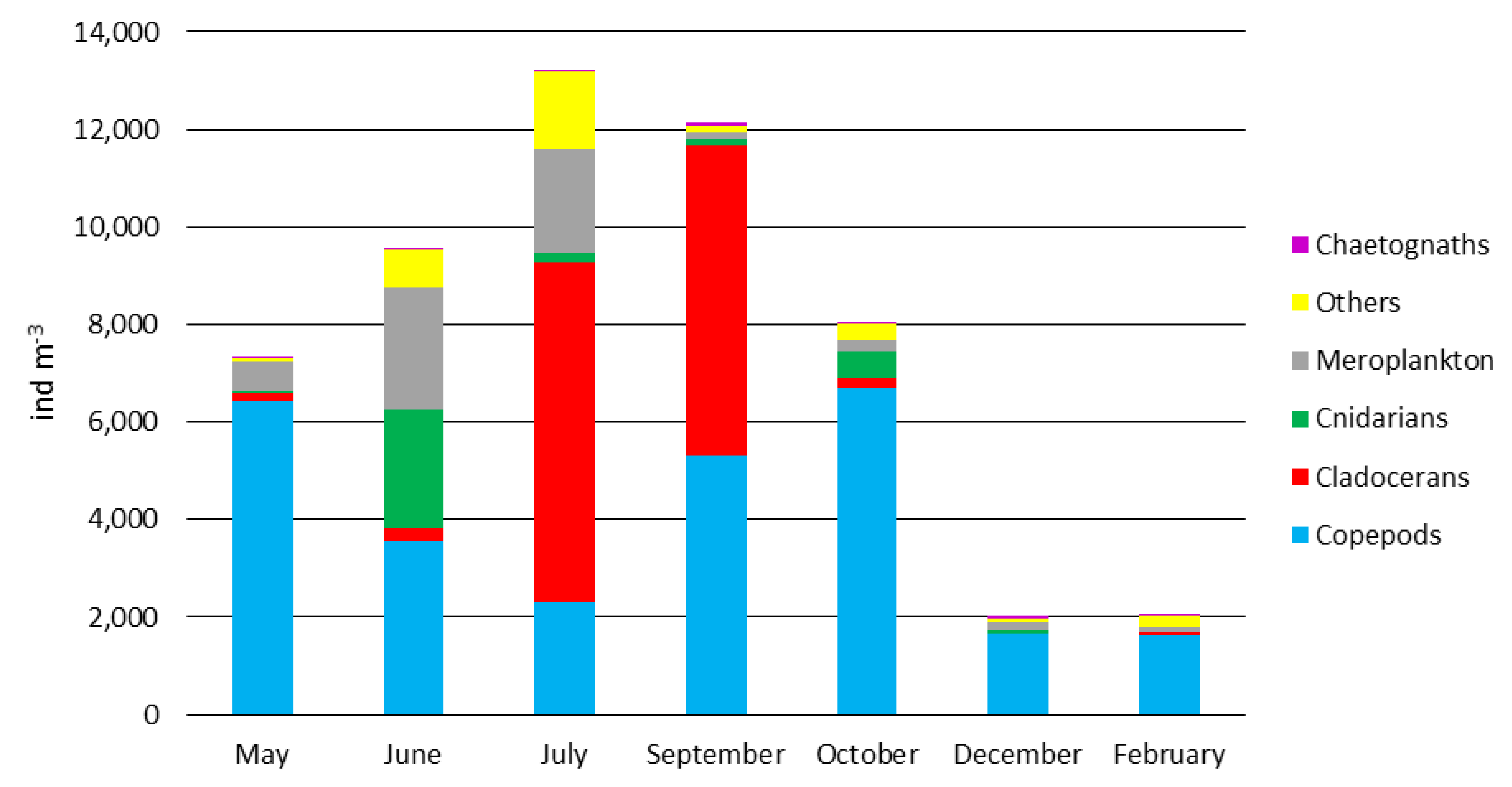
3.1. Temperature and Mesozooplankton in the Field
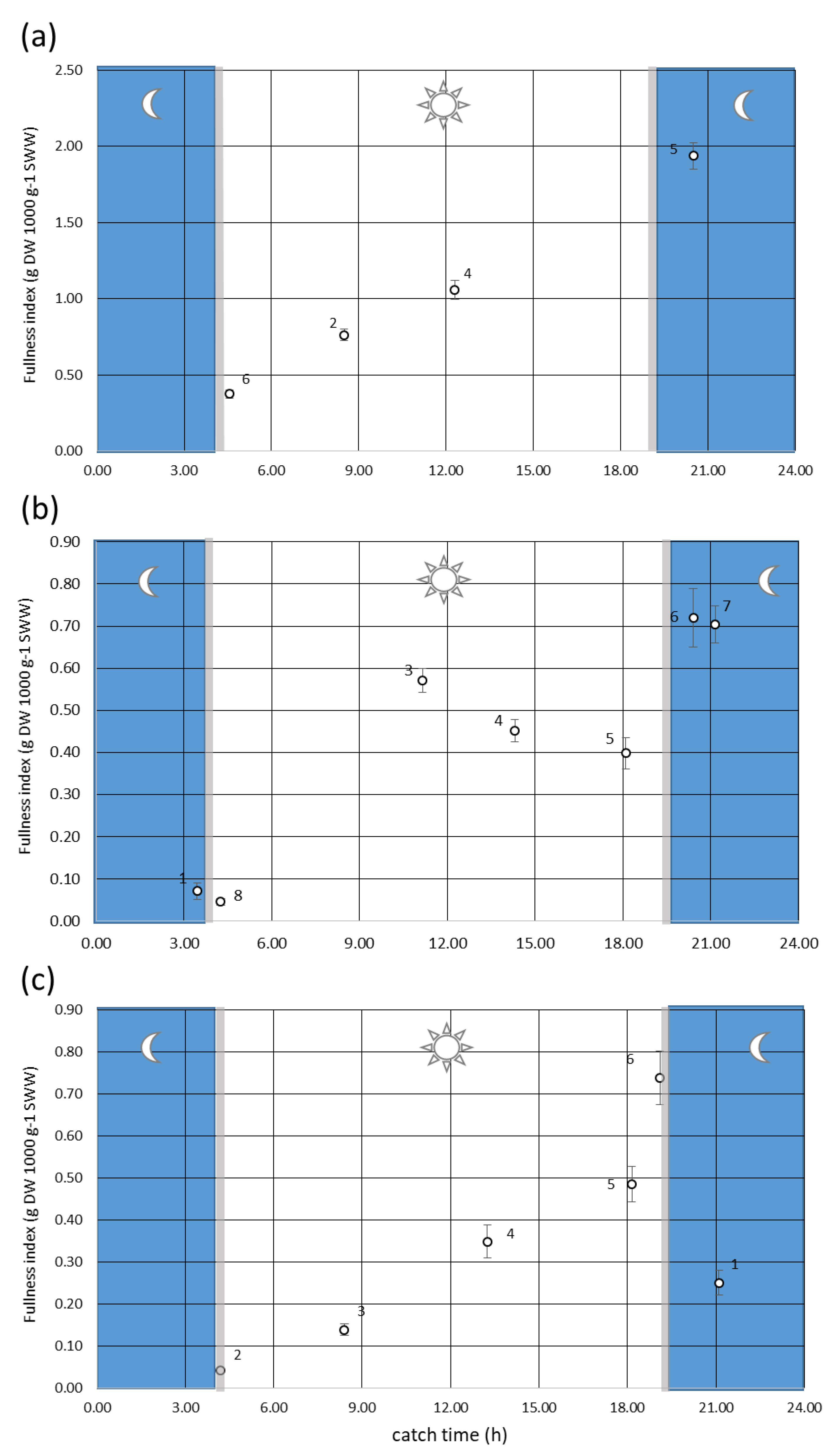
3.2. Diel Feeding Cycle
3.3. Composition of the Diet
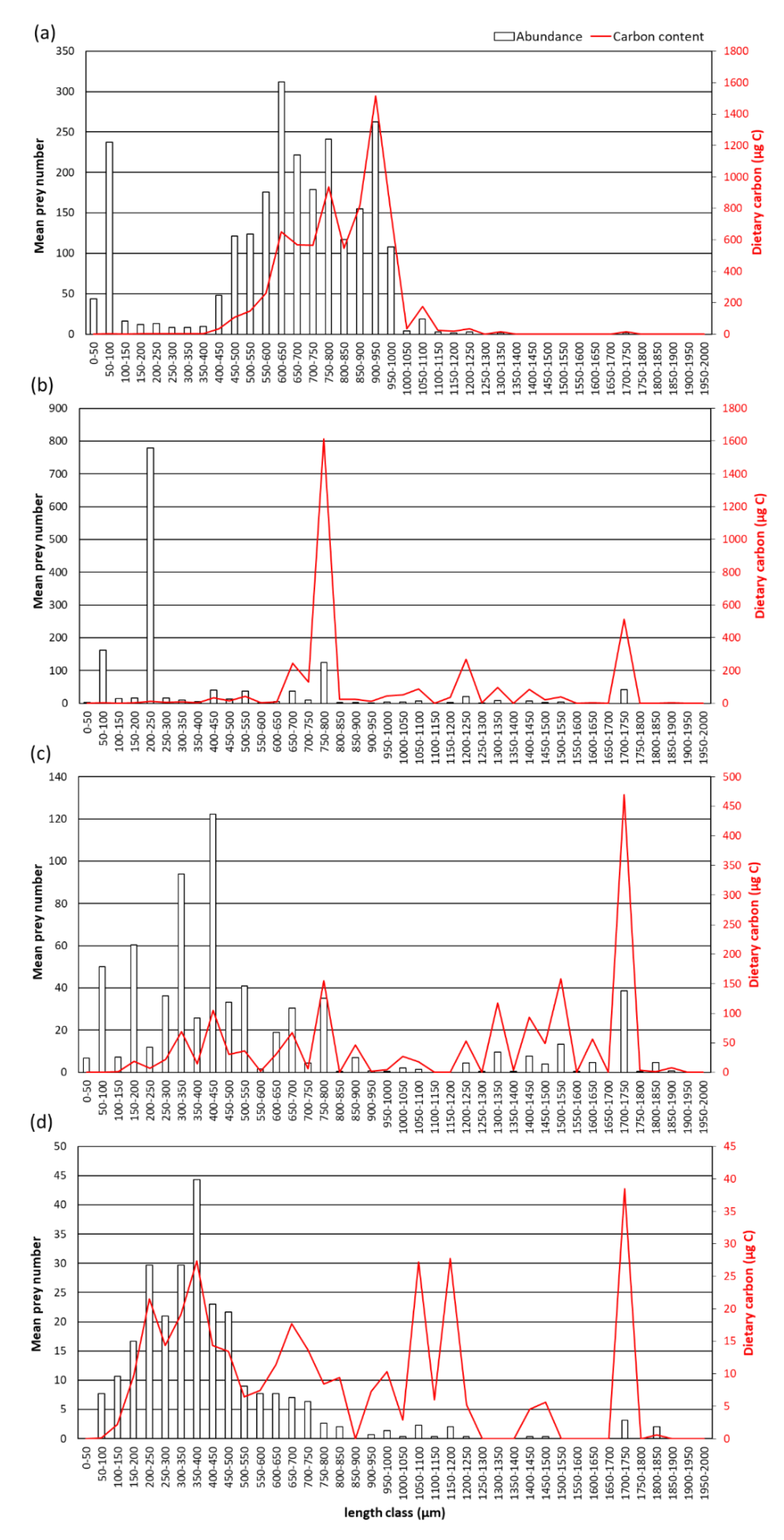
3.4. Food Carbon
3.5. Selection of the Prey
4. Discussion
4.1. Trophic Environment
4.2. Diel Feeding Cycle
4.3. Diet Composition and Seasonality
4.4. Dietary Carbon
4.5. Feeding Selectivity
Author Contributions
Funding
Institutional Review Board Statement
Informed Consent Statement
Data Availability Statement
Acknowledgments
Conflicts of Interest
Appendix A

| Prey item |
|
| References |
|---|---|---|---|
| Cocconeis spp. Coscinodiscus spp. Diploneis spp. Paralia sulcata Pleurosigma spp. Nitzschia spp. Thalassiosira spp. Pennate diatom | volume | C = V × 0.11 | (a) [75,76]; (b) [77] |
| Ceratium candelabrum Ceratium furca Ceratium trichoceros Ceratium tripos Ceratium spp. Diplopsalis spp. Dinophysis caudata Dinophysis fortii Dinophysis sacculus Gonyaulax polygramma Gonyaulax spp. Katodinium spp. Lingulodinium polyedrum Phalacroma spp. Podolampas palmipes Prorocentrum micans Protoperidinium claudicans Protoperidinium conicum Protoperidinium crassipes Protoperidinium depressum Protoperidinium divergens Protoperidinium oblongum Protoperidinium oceanicum Protoperidinium steinii Ornithocercus magnificus Scrippsiella spp. Protoperidinium spp. | volume | C = V × 0.13 | (a) [75,76]; (b) [77] |
| Codonellopsis schabi Eutintinnus fraknoii Stenosemella ventricosa Tintinnopsis radix | volume | C = (444.5 + 0.053 × V) × 10−6 | (b) [78] |
| Gastropoda pediveliger | direct weight | C = (DW × 31.25)/100 | (b) [55] |
| Bivalvia veliger | direct weight | C = (DW × 31.25)/100 | (a) [79]; (b) [55] |
| Polychaeta larvae | direct weight | C = (DW × 40)/100 | (a) [79]; (b) [80] |
| Evadne nordmanni Evadne spinifera Penilia avirostris Pleopis polyphemoides Podon intermedius Podonidae | direct weight | C = (DW × 33.1)/100 | (a) [81]; (b) [82] |
| Acartia clausi Acartia tonsa Acartia spp. | Log C = 3.032 Log PL − 8.556 | (b) [83] | |
| Calanus spp. (ref. Calanus helgolandicus) | Log DW = 2.691 Log PL − 6.883 | C = 0.372 DW − 0.248 | (a) [84]; (b) [85] |
| Centropages ponticus Centropages typicus Centropages spp. | Log DW = 2.451 Log PL − 6.103 | C = (DW × 37.6)/100 | (a) [84]; (b) [82] |
| Clausocalanus sp. Paracalanus parvus Paracalanus spp. Clauso-Paracalanidae Calanoida indet. | Log C = 3.128 Log PL − 8.451 | (b) [86] | |
| Nannocalanus minor (rif. Calanus helgolandicus) | Log DW = 2.691 Log PL − 6.883 | C = 0.372 DW − 0.248 | (a) [84]; (b) [85] |
| Temora longicornis | Log DW = 3.059 Log PL − 7.682 | C = (DW × 46.8)/100 | (a) [84]; (b) [87] |
| Temora stylifera | (Log DW = 2.71 Log L − 3.685)/1000 | C = (DW × 46.8)/100 | (a) [88]; (b) [87] |
| Oithona nana Oithona cf. nana Oithona plumifera Oithona cf. plumifera Oithona setigera Oithona cf. similis Oithona spp. | C = 9.4676 10−7 PL2.16 | (b) [89] | |
| Corycaeus spp. (ref. Cyclopoida) | Ln DW = 1.96 Ln PL − 11.64 | C = (DW × 43.1)/100 | (a) [90]; (b) [87] |
| Oncaea spp. | direct weight | C = (DW × 38.2)/100 | (a) (b) [87] |
| Clytemnestra scutellata | Ln DW = 1.96 Ln PL − 11.64 | C = (DW × 42.4)/100 | (a) [90]; (b) [91] |
| Euterpina acutifrons | DW = 1.389 10−8 L2.857 | C = (DW × 46)/100 | (a) (b) [92] |
| Microsetella rosea Harpacticoida indet. (ref. Microsetella norvegica) | C = 2.65 10−6 L1.95 | (b) [93] | |
| Copepoda eggs | 4/3 π (L/2)3 | C = 140 × 10−9 × V | (b) [94] |
| Copepod nauplii (ref. Acartia nauplii) | Log DW = 2.848 Log L − 7.265 | C = (DW × 42.4)/100 | (a) [95]; (b) [91] |
| Cirripedia nauplii | DW = 80.627 × L4.27 | C = (DW × 39.97)/100 | (a) [55]; (b) [96] |
| Cirripedia cypris | direct weight | C = (DW × 39.97)/100 | (b) [96] |
| Squilla mantis alima (ref. Lucifer reynaudii) | direct weight | C = (DW × 41.1)/100 | (a) (b) [97] |
| Hyperiidae indet. Porcellana zoeae Decapoda zoeae Decapoda mysis Decapoda phyllosoma | direct weight | C = (DW × 43.69)/100 | (a) [79]; (b) [87] |
| Decapoda nauplii (ref. Cirripedia larvae) | direct weight | (a) [98] | |
| Oikopleura spp. | C = 0.04 × L3.29 | (b) [99] | |
| Chaetognatha (ref. Sagitta elegans) | DW = 0.114 × L3.1963 | C = (DW × 35.8)/100 | (a) (b) [100] |
| Engraulis encrasicolus eggs Teleostea spheric eggs (ref. Engraulis mordax) | direct weight | C = 0.457 × DW | (a) [101]; (b) [102] |
| Teleostea larvae (ref. E. encrasicolus larvae) | DW = 6 × 10⁻¹⁵ L4.1229 | C = 0.457 × DW | (a) [58]; (b) [102] |
| Invertebrata spheric eggs (ref. Copepoda eggs) | 4/3 π (L/2)3 | C = 140 × 10−9 × V | (b) [94] |
| Invertebrata elliptical eggs (ref. Copepoda eggs) | 4/3 π (L/2) × (L/4)2 | C = 140 × 10−9 × V | (b) [94] |
| Date | 10 May 06 | 20 June 06 | 26 July 06 | 04 Sept 06 | 26 Oct 06 | 14 Dec 06 | 01 Feb 07 | |
|---|---|---|---|---|---|---|---|---|
| Time | 22:30 | 21:30 | 18:50 | 16:50 | 17:50 | 15:20 | 18:50 | |
| Group | Sampling depth (m) | 16 | 16 | 16 | 17 | 20 | 12 | 22 |
| Dinophyceae | Noctiluca scintillans | 0 | 20 | 286 | 74 | 0 | 30 | 88 |
| Hydrozoa | Anthomedusae indet. | 27 | 27 | 20 | 85 | 0 | 0 | 0 |
| Obelia spp. | 0 | 12 | 4 | 0 | 6 | 0 | 4 | |
| Leptomedusae indet. | 0 | 4 | 0 | 0 | 0 | 0 | 0 | |
| Siphonophorae | Muggiaea spp. | 0 | 220 | 0 | 0 | 0 | 0 | 0 |
| Siphonophorae indet. | 14 | 2141 | 192 | 41 | 527 | 37 | 16 | |
| Hydrozoa indet. | 0 | 0 | 0 | 0 | 0 | 1 | 0 | |
| Scyphozoa | Scyphozoa ephyrae | 0 | 0 | 0 | 0 | 0 | 1 | 0 |
| Anthozoa | Cerianthus larvae | 0 | 0 | 0 | 0 | 0 | 0 | 1 |
| Ctenophora | Ctenophora larvae | 10 | 31 | 0 | 0 | 0 | 0 | 0 |
| Ctenophora indet. | 0 | 0 | 0 | 0 | 0 | 4 | 1 | |
| Nemertea | Nemertea pilidia | 0 | 20 | 0 | 0 | 0 | 0 | 0 |
| Phoronida | Phoronida actinotrochae | 2 | 0 | 0 | 0 | 0 | 0 | 0 |
| Gastropoda | Creseis clava | 0 | 0 | 0 | 0 | 3 | 4 | 0 |
| Gastropoda pediveligers | 239 | 408 | 455 | 0 | 13 | 60 | 17 | |
| Bivalvia | Bivalvia veligers | 6 | 67 | 357 | 37 | 110 | 98 | 34 |
| Polychaeta | Polychaeta larvae | 0 | 12 | 16 | 18 | 56 | 25 | 4 |
| Polychaeta indet. | 24 | 106 | 0 | 0 | 0 | 0 | 0 | |
| Branchiopoda | Pleopis polyphaemoides | 2 | 24 | 35 | 4 | 0 | 0 | 37 |
| Podon intermedius | 2 | 16 | 20 | 0 | 6 | 0 | 10 | |
| Evadne nordmanni | 78 | 8 | 251 | 129 | 0 | 0 | 0 | |
| Evadne spinifera | 73 | 192 | 43 | 122 | 9 | 0 | 0 | |
| Evadne tergestina | 0 | 12 | 78 | 0 | 0 | 0 | 0 | |
| Podonidae indet. | 0 | 0 | 0 | 0 | 3 | 0 | 0 | |
| Penilia avirostris | 0 | 20 | 6533 | 6097 | 198 | 16 | 1 | |
| Ostracoda | Ostracoda indet. | 0 | 8 | 0 | 4 | 0 | 0 | 1 |
| Calanoida | Acartia (Acartiura) clausi | 345 | 298 | 145 | 89 | 41 | 22 | 11 |
| Acartia juv. | 388 | 200 | 184 | 26 | 116 | 93 | 17 | |
| Anomalocera sp. | 2 | 0 | 0 | 0 | 0 | 0 | 0 | |
| Calanus helgolandicus | 200 | 0 | 0 | 0 | 0 | 3 | 10 | |
| Calocalanus spp. | 2 | 0 | 0 | 4 | 0 | 0 | 0 | |
| Candacia juv. | 0 | 0 | 0 | 0 | 0 | 0 | 1 | |
| Centropages ponticus | 39 | 4 | 0 | 7 | 0 | 0 | 0 | |
| Centropages typicus | 86 | 0 | 0 | 0 | 0 | 0 | 0 | |
| Centropages spp. | 839 | 525 | 24 | 81 | 0 | 0 | 0 | |
| Clausocalanus arcuicornis | 6 | 0 | 0 | 7 | 0 | 3 | 30 | |
| Clausocalanus furcatus | 2 | 0 | 0 | 59 | 72 | 0 | 13 | |
| Clausocalanus juv. | 51 | 8 | 8 | 85 | 144 | 3 | 54 | |
| Ctenocalanus vanus | 114 | 0 | 0 | 0 | 0 | 4 | 448 | |
| Diaixis pygmaea | 0 | 0 | 0 | 0 | 0 | 8 | 110 | |
| Euchaeta hebes | 0 | 0 | 0 | 0 | 0 | 0 | 1 | |
| Mecynocera clausi | 0 | 0 | 0 | 4 | 0 | 0 | 0 | |
| Paracalanus denudatus | 649 | 8 | 0 | 55 | 0 | 0 | 0 | |
| Paracalanus parvus s.l. | 2110 | 1173 | 702 | 1358 | 1239 | 150 | 317 | |
| Pseudocalanus elongatus | 120 | 0 | 0 | 0 | 0 | 0 | 0 | |
| Temora longicornis | 171 | 4 | 12 | 0 | 0 | 0 | 3 | |
| Temora stylifera | 2 | 0 | 24 | 1517 | 370 | 41 | 17 | |
| Calanoida copepodites | 739 | 545 | 553 | 698 | 618 | 169 | 147 | |
| Cyclopoida | Oithona nana | 51 | 459 | 75 | 140 | 85 | 34 | 6 |
| Oithona plumifera | 0 | 0 | 4 | 85 | 72 | 33 | 19 | |
| Oithona setigera | 0 | 4 | 4 | 0 | 0 | 0 | 0 | |
| Oithona similis | 153 | 0 | 4 | 15 | 13 | 3 | 3 | |
| Oithona spp. | 200 | 118 | 71 | 114 | 72 | 255 | 33 | |
| Ergasilida | Corycaeidae indet. | 27 | 4 | 35 | 103 | 348 | 170 | 77 |
| Oncaea spp. | 6 | 102 | 267 | 572 | 3250 | 531 | 257 | |
| Sapphirina spp. | 0 | 0 | 0 | 0 | 0 | 1 | 0 | |
| Harpacticoida | Clytemnestra scutellata | 0 | 0 | 0 | 0 | 0 | 1 | 0 |
| Euterpina acutifrons | 4 | 4 | 125 | 225 | 191 | 77 | 36 | |
| Harpacticoida indet. | 2 | 35 | 8 | 4 | 0 | 1 | 0 | |
| Copepoda | Copepoda nauplii | 122 | 78 | 59 | 78 | 63 | 60 | 26 |
| Cirripedia | Cirripedia nauplii | 39 | 8 | 75 | 0 | 13 | 1 | 1 |
| Isopoda | Epicaridea indet. | 0 | 0 | 0 | 0 | 3 | 0 | 3 |
| Decapoda | Pisidia larvae | 0 | 12 | 0 | 0 | 0 | 0 | 0 |
| Brachiura zoea | 0 | 0 | 0 | 4 | 0 | 0 | 1 | |
| Decapoda mysis | 2 | 98 | 43 | 44 | 25 | 4 | 1 | |
| Decapoda zoea | 14 | 12 | 4 | 18 | 3 | 0 | 4 | |
| Decapoda nauplii | 0 | 0 | 4 | 0 | 0 | 0 | 0 | |
| Mysida | Mysida indet. | 2 | 0 | 8 | 0 | 3 | 0 | 1 |
| Cumacea | Cumacea indet. | 0 | 0 | 0 | 0 | 0 | 0 | 1 |
| Chaetognatha | Sagitta spp. | 4 | 39 | 35 | 48 | 13 | 78 | 44 |
| Echinodermata | Asteroidea larvae | 0 | 0 | 27 | 0 | 0 | 0 | 0 |
| Psammechinus larvae | 14 | 4 | 8 | 0 | 0 | 0 | 0 | |
| Echinoidea plutei | 135 | 1733 | 1012 | 4 | 6 | 5 | 41 | |
| Holothuroidea auricularia | 108 | 47 | 16 | 0 | 0 | 0 | 0 | |
| Echinodermata plutei | 39 | 4 | 0 | 0 | 0 | 0 | 0 | |
| Hemichordata | Hemichordata tornariae | 0 | 0 | 0 | 0 | 0 | 0 | 1 |
| Appendicularia | Oikopleura spp. | 39 | 557 | 1259 | 63 | 314 | 16 | 117 |
| Thaliacea | Doliolum spp. | 0 | 47 | 35 | 0 | 19 | 4 | 4 |
| Cephalochordata | Branchiostoma lanceolatum juv. | 0 | 43 | 0 | 0 | 0 | 0 | 0 |
| Vertebrata | Osteichthyes eggs | 14 | 27 | 35 | 4 | 6 | 0 | 0 |
| Osteichthyes larvae | 4 | 31 | 59 | 4 | 3 | 0 | 1 | |
| TOTAL | 7320 | 9576 | 13,212 | 12,125 | 8035 | 2044 | 2075 |
References
- Bakun, A. Wasp-waist populations and marine ecosystem dynamics: Navigating the ‘predator pit’ topographies. Prog. Oceanogr. 2006, 68, 271–288. [Google Scholar] [CrossRef]
- Coll, M.; Shannon, L.J.; Moloney, C.L.; Palomera, I.; Tudela, S. Comparing trophic flows and fishing impacts of a NW Mediterranean ecosystem with coastal upwelling systems by means of standardized models and indicators. Ecol. Modell. 2006, 198, 53–70. [Google Scholar] [CrossRef]
- Alheit, J.; Roy, C.; Kifani, S. Decadal-scale variability in populations. In Climate Change and Small Pelagic Fish; Checkley, D.M., Jr., Alheit, J., Oozeki, Y., Roy, C., Eds.; Cambridge University Press: Cambridge, UK, 2009; pp. 64–87. [Google Scholar]
- Van der Lingen, C.D.; Bertrand, A.; Bode, A.; Brodeur, R.; Cubillos, L.A.; Espinoza, P.; Friedland, K.; Garrido, S.; Irigoien, X.; Miller, T.; et al. Trophic dynamics. In Climate Change and Small Pelagic Fish; Checkley, D., Roy, C., Alheit, J., Oozeki, Y., Eds.; Cambridge University Press: Cambridge, UK, 2009; pp. 112–157. [Google Scholar]
- Costalago, D.; Palomera, I.; Tirelli, V. Seasonal comparison of the diets of juvenile European anchovy Engraulis encrasicolus and sardine Sardina pilchardus in the Gulf of Lions. J. Sea Res. 2014, 89, 64–72. [Google Scholar] [CrossRef]
- Chen, C.T.; Carlotti, F.; Harmelin-Vivien, M.; Guilloux, L.; Bănaru, D. Temporal variation in prey selection by adult European sardine (Sardina pilchardus) in the NW Mediterranean Sea. Progr. Oceanogr. 2021, 196, 102617. [Google Scholar] [CrossRef]
- Brosset, P.; Le Bourg, B.; Costalago, D.; Bănaru, D.; Van Beveren, E.; Bourdeix, J.H.; Fromentin, J.M.; Ménard, F.; Saraux, C. Linking small pelagic dietary shifts with ecosystem changes in the Gulf of Lions. Mar. Ecol. Progr. Ser. 2016, 554, 157–171. [Google Scholar] [CrossRef]
- Saraux, C.; Van Beveren, E.; Brosset, P.; Queiros, Q.; Bourdeix, J.-H.; Dutto, G.; Gasset, E.; Jac, C.; Bonhommeau, S.; Fromentin, J.-M. Small pelagic fish dynamics: A review of mechanisms in the Gulf of Lions. Deep.-Sea Res. Pt. II 2019, 159, 52–61. [Google Scholar] [CrossRef]
- Ryther, J.H. Photosynthesis and fish production in the sea. Science 1969, 166, 72–76. [Google Scholar] [CrossRef]
- Walsh, J.J. A carbon budget for overfishing off Peru. Nature 1981, 290, 300–304. [Google Scholar] [CrossRef]
- Garrido, S.; Marçalo, A.; Zwolinski, J.; van der Lingen, C.D. Laboratory investigations on the effect of prey size and concentration on the feeding behaviour of Sardina pilchardus. Mar. Ecol. Progr. Ser. 2007, 330, 189–199. [Google Scholar] [CrossRef]
- James, A.G. Are clupeoid microphagists herbivorous or omnivorous? A review of the diets of some commercially important clupeids. S. A. J. Mar. Sci. 1988, 7, 161–177. [Google Scholar] [CrossRef]
- Andreu, B. Las branquispinas en la caracterización de las poblaciones de Sardina pilchardus. (Walb.) Inv. Pesq. 1969, 33, 425–607. [Google Scholar]
- Palomera, I.; Olivar, P.; Salat, J.; Sabatés, A.; Coll, M.; García, A.; Morales-Nin, B. Small pelagic fish in the NW Mediterranean Sea: An ecological review. Progr. Oceanogr. 2007, 74, 377–396. [Google Scholar] [CrossRef]
- Costalago, D.; Garrido, S.; Palomera, I. Comparison of the feeding apparatus and diet of European sardines Sardina pilchardus of Atlantic and Mediterranean waters: Ecological implications. J. Fish Biol. 2015, 86, 1348–1362. [Google Scholar] [CrossRef]
- Nikolioudakis, N.; Palomera, I.; Machias, A.; Somarakis, S. Diel feeding intensity and daily ration of the sardine Sardina pilchardus. Mar. Ecol. Progr. Ser. 2011, 437, 215–228. [Google Scholar] [CrossRef]
- Nikolioudakis, N.; Isari, S.; Pitta, P.; Somarakis, S. Diet of sardine Sardina pilchardus: An “end-to-end” field study. Mar. Ecol. Progr. Ser. 2012, 453, 173–188. [Google Scholar] [CrossRef]
- Costalago, D.; Navarro, J.; Álvarez-Calleja, I.; Palomera, I. Ontogenetic and seasonal changes in the feeding habits and trophic levels of two small pelagic fish species. Mar. Ecol. Progr. Ser. 2012, 460, 169–181. [Google Scholar] [CrossRef]
- Costalago, D.; Palomera, I. Feeding of European pilchard (Sardina pilchardus) in the northwestern Mediterranean: From late larvae to adults. Sci. Mar. 2014, 78, 41–54. [Google Scholar] [CrossRef]
- Albo-Puigserver, M.; Borme, D.; Coll, M.; Tirelli, V.; Palomera, I.; Navarro, J. Trophic ecology of range-expanding round sardinella and resident sympatric species in the NW Mediterranean. Mar. Ecol. Progr. Ser. 2019, 620, 139–154. [Google Scholar] [CrossRef]
- Sever, T.M.; Bayhan, B.; Taskavak, E. A preliminary study on the feeding regime of european pilchard (Sardina pilchardus Walbaum1792) in Izmir Bay, Turkey, Eastern Aegean Sea. NAGA WorldFish Cent. Q. 2005, 28, 41–48. [Google Scholar]
- Nikolioudakis, N.; Isari, S.; Somarakis, S. Trophodynamics of anchovy in a non-upwelling system: Direct comparison with sardine. Mar. Ecol. Progr. Ser. 2014, 500, 215–229. [Google Scholar] [CrossRef]
- Vučetić, T. Ishrana odrasle srdele (Sardina pilchardus Walb.) u srednjem Jadranu. Acta Adriat. 1963, 10, 3–43. [Google Scholar]
- Vučetić, T. O odnosu srdele (Sardina pilchardus Walb.) prema biotskim faktorima sredine–zooplanktonu. Acta Adriat. 1964, 11, 269–276. [Google Scholar]
- Zorica, B.; Keč, V.Č.; Vidjak, O.; Mladineo, I.; Balić, D.E. 2016 Feeding habits and helminth parasites of sardine (S. pilchardus) and anchovy (E. encrasicolus) in the Adriatic Sea. Mediterr. Mar. Sci. 2016, 17, 216–229. [Google Scholar] [CrossRef]
- Zorica, B.; Keč, V.Č.; Vidjak, O.; Kraljević, V.; Brzulja, G. Seasonal pattern of population dynamics, spawning activities, and diet composition of sardine (Sardina pilchardus Walbaum) in the eastern Adriatic Sea. Turk. J. Zool. 2017, 41, 892–900. [Google Scholar] [CrossRef]
- Malačič, V.; Celio, M.; Čermelj, B.; Bussani, A.; Comici, C. Interannual evolution of seasonal thermohaline properties in the Gulf of Trieste (Northern Adriatic) 1991-2003. J. Geophys. Res. 2006, 111, C08009. [Google Scholar] [CrossRef]
- Stambler, N. The Mediterranean Sea—Primary productivity. In The Mediterranean Sea: Its History and Present Challenges; Goffredo, S., Dubinsky, Z., Eds.; Springer: Berlin/Heidelberg, Germany, 2014; pp. 113–121. [Google Scholar]
- Grilli, F.; Accoroni, S.; Acri, F.; Aubry, F.B.; Bergami, C.; Cabrini, M.; Campanelli, A.; Giani, M.; Guicciardi, S.; Marini, M.; et al. Seasonal and Interannual Trends of Oceanographic Parameters over 40 Years in the Northern Adriatic Sea in Relation to Nutrient Loadings Using the EMODnet Chemistry Data Portal. Water 2020, 12, 2280. [Google Scholar] [CrossRef]
- Santojanni, A.; Leonori, I.; Piccinetti, C.; Fabi, G.; Angelini, S.; Belardinelli, A.; Biagiotti, I.; Canduci, G.; Carpi, P.; Colella, S.; et al. GSA 17—Mare Adriatico settentrionale e centrale. In Annuario Sullo Stato Delle Risorse e Sulle Strutture Produttive dei Mari italiani. Biologia Marina Mediterranea; Mannini, A., Sabatella, R.F., Eds.; Erredi: Genova, Italy, 2015; Volume 22, (Suppl. 1), pp. 116–146. [Google Scholar]
- Vasilakopoulos, P.; Maravelias, C.D.; Tserpes, G. The alarming decline of Mediterranean fish stocks. Curr. Biol. 2014, 24, 1643–1648. [Google Scholar] [CrossRef]
- Mosetti, F. Condizioni idrologiche della costiera triestina. Hydrores 1988, 6, 29–38. [Google Scholar]
- Cozzi, S.; Falconi, C.; Comici, C.; Cermelj, B.; Kovac, N.; Turk, V.; Giani, M. Recent evolution of river discharges in the Gulf of Trieste and their potential response to climate changes and anthropogenic pressure. Est. Coast. Shelf Sci. 2012, 115, 14–24. [Google Scholar] [CrossRef]
- Ivlev, V.S. Experimental Ecology of the Feeding of Fishes; Scott, D., Translator; Yale University Press: New Haven, CT, USA, 1961; p. 302. [Google Scholar]
- Škrivanić, A.; Zavodnik, D. Migrations of the sardine (Sardina pilchardus) in relation to hydrographical conditions of the Adriatic Sea. Neth. J. Sea Res. 1973, 7, 7–18. [Google Scholar] [CrossRef]
- Gamulin, T.; Hure, J. Spawning of the sardine at a definite time of day. Nature 1956, 177, 193–194. [Google Scholar] [CrossRef]
- Tičina, V.; Ivančić, I.; Emrić, V. Relation between the hydrographic properties of the northern Adriatic Sea water and sardine (Sardina pilchardus) population schools. Period. Biolog. 2000, 102, 181–192. [Google Scholar]
- Gamulin, T. La ponte et les aires de ponte de la sardine (Sardina pilchardus Walb.) dans l’Adriatique de 1947 à 1950. In Report of “HVAR” Expedition 4 (4 C); Springer: Berlin/Heidelberg, Germany, 1954; pp. 1–66. [Google Scholar]
- Hure, J. Distribution annuelle vertical du zooplankton sur une station de l’Adriatique méridionale. Acta Adriat. 1955, 7, 1–72. [Google Scholar]
- Hure, J. Dnevna migracija i sezonska vertikalna raspodjela zooplanktona dubljeg mora. Acta Adriat. 1961, 9, 1–59. [Google Scholar]
- Hure, J. Rythme saisonnier de la distribution vertical du zooplancton dams les eaux profondes de l’Adriatique meridionale. Acta Adriat. 1964, 11, 167–172. [Google Scholar]
- Vučetić, T. Vertikalna raspodjela zooplanktona u Velikom jezeru otoka Mljeta. Acta Adriat. 1961, 6, 1–20. [Google Scholar]
- Mužinić, R. Migrations of adult sardines in the central Adriatic. Neth. J. Sea Res. 1973, 7, 19–30. [Google Scholar] [CrossRef]
- Pierson, J.; Camatti, E.; Hood, R.; Kogovšek, T.; Lučić, D.; Tirelli, V.; Malej, A. Mesozooplankton and gelatinous zooplankton in the face of environmental stressors. In Coastal Ecosystems in Transition: A Comparative Analysis of the Northern Adriatic and Chesapeake Bay, 1st ed.; Malone, T., Malej, A., Faganeli, J., Eds.; Geophysical Monograph; Wiley & Sons Ltd.: Hoboken, NJ, USA, 2021; Volume 256, pp. 105–127. [Google Scholar] [CrossRef]
- Borme, D.; Tirelli, V.; Palomera, I. Feeding habits of European pilchard late larvae in a nursery area in the Adriatic Sea. J. Sea Res. 2013, 78, 8–17. [Google Scholar] [CrossRef]
- Zaret, T.M. Predators, invisible prey, and the nature of polymorphism in the Cladocera (Class Crustacea). Limnol. Oceanogr. 1972, 17, 171–184. [Google Scholar] [CrossRef]
- Janssen, J. Searching for zooplankton just outside Snell’s window. Limnol. Oceanogr. 1981, 26, 1168–1171. [Google Scholar] [CrossRef]
- Varela, M.; Alvarez-Ossorio, M.T.; Valdéz, L. Método para el estudio cuantitativo del contenido estomacal de la sardina. Resultados preliminares. Bol. Instit. Esp. Oceanogr. 1990, 6, 117–126. [Google Scholar]
- Garrido, S.; Ben-Hamadou, R.; Oliveira, P.B.; Cunha, M.E.; Chícharo, M.A.; van der Lingen, C.D. Diet and feeding intensity of sardine Sardina pilchardus: Correlation with satellite derived chlorophyll data. Mar. Ecol. Progr. Ser. 2008, 354, 245–256. [Google Scholar] [CrossRef]
- Massutì, M.; Oliver, M. Estudio de la biometria y biologia de la sardine de Mahón (Baleares), especialmente de su alimentación. Bol. Instit. Esp. Oceanogr. 1948, 3, 1–15. [Google Scholar]
- Varela, M.; Larrañaga, A.; Costas, E.; Rodriguez, B. Contenido estomacal de la sardina (Sardina pilchardus Walbaum) durante la campaña Saracus 871 en la plataformas Cantábrica y de Galicia en febrero de 1971. Bol. Instit. Esp. Oceanogr. 1988, 5, 17–28. [Google Scholar]
- Cunha, M.E.; Garrido, S.; Pissarra, J. The use of stomach fullness and colour indices to assess Sardina pilchardus feeding. J. Mar. Biol. Ass. 2005, 85, 425–431. [Google Scholar] [CrossRef]
- Silva, E. Some notes on the food of the pilchard Sardina pilchardus (Walb.), of the Portuguese coast. Rev. De La Fac. De Cienc. De Lisb. 2 Ser. 1954, 4, 281–294. [Google Scholar]
- Davies, D.H. The South African pilchard (Sardinops ocellata). Preliminary report on feeding off the West Coast, 1953–1956. Inv. Rep. Div. Fish. S. A. 1957, 30, 40. [Google Scholar]
- James, A.G. Feeding ecology, diet and field-based studies on feeding selectivity of the Cape anchovy Engraulis capensis Gilchrist, 1913. S. Afr. J. Mar. Sci. 1987, 5, 673–692. [Google Scholar] [CrossRef]
- Van der Lingen, C.D. Diet of sardine Sardinops sagax in the southern Benguela upwelling ecosystem. S. Afr. J. Mar. Sci. 2002, 24, 301–316. [Google Scholar] [CrossRef]
- Bode, A.; Carrera, P.; Lens, S. The pelagic foodweb in the upwelling ecosystem of Galicia (NW Spain) during spring: Natural abundance of stable carbon and nitrogen isotopes. ICES J. Mar. Sci. 2003, 60, 11–22. [Google Scholar] [CrossRef]
- Borme, D.; Tirelli, V.; Brandt, S.B.; Umani, S.F.; Arneri, E. Diet of Engraulis encrasicolus in the northern Adriatic Sea (Mediterranean): Ontogenetic changes and feeding selectivity. Mar. Ecol. Progr. Ser. 2009, 392, 193–209. [Google Scholar] [CrossRef]
- Tudela, S.; Palomera, I. Trophic ecology of the European anchovy Engraulis encrasicolus in the Catalan Sea (northwest Mediterranean). Mar. Ecol. Progr. Ser. 1997, 160, 121–134. [Google Scholar] [CrossRef]
- Green, E.P.; Dagg, M.J. Mesozooplankton associations with medium to large marine snow aggregates in the northern Gulf of Mexico. J. Plankton Res. 1997, 19, 435–447. [Google Scholar] [CrossRef]
- Diaz, E.; Cotano, U.; Villate, F. Reproductive response of Euterpina acutifrons in 2 estuaries of the Basque Country (Bay of Biscay) with contrasting nutritional environment. J. Exp. Mar. Biol. Ecol. 2003, 292, 213–230. [Google Scholar] [CrossRef]
- Štirn, J. The north Adriatic pelagial, its oceanological characteristics, structure and distribution of the biomass during the year 1965. Diss. Acad. Sci. Arts Slov. 1969, 12, 1–92. [Google Scholar]
- Specchi, M.; Orlandi, C.; Radin, B.; Manetti, M.F.; Cassetti, P. Observations on the occurrence of Penilia avirostris Dana and the eggs of Engraulis encrasicolus L. in the Gulf of Trieste (Northern Adriatic Sea). Boll. Soc. Adr. Sci. 1999, 78, 309–316. [Google Scholar]
- Ogawa, Y.; Nakahara, T. Interrelationships between pelagic fishes and plankton in the coastal fishing ground of the southwestern Japan Sea. Mar. Ecol. Progr. Ser. 1979, 1, 115–122. [Google Scholar] [CrossRef]
- Zaret, T.M. The effect of prey motion on planktivore choice. In Evolution and Ecology of Zooplankton Communities; Kerfoot, W.C., Ed.; New England University Press: Hanover, NH, USA, 1980; pp. 599–603. [Google Scholar]
- Wright, D.I.; O’Brien, W.J. Differential location of Chaoborus larvae and Daphnia by fish: The importance of motion and visible size. Am. Mid. Nat. 1982, 108, 68–73. [Google Scholar] [CrossRef]
- Imbrahim, A.A.; Huntingford, F.A. Laboratory and field studies on diet choice of three-spined thicklebacks, Gasterosteus aculeatus L., in relation to profitability and visual features of prey. J. Fish Biol. 1989, 34, 245–258. [Google Scholar] [CrossRef]
- Luecke, C.; O’Brien, W.J. Prey location volume of a planktivorous fish: A new measurement of prey vulnerability. Can. J. Fish. Aquat. Sci. 1981, 38, 1264–1270. [Google Scholar] [CrossRef]
- Vinyard, G.L.; O’Brien, W.J. Effects of light and turbidity on the reactive distance of bluegill (Lepomis macrochirus). J. Fish. Res. Board Can. 1976, 33, 2845–2849. [Google Scholar] [CrossRef]
- Strickler, J.R.; Udvadia, A.J.; Marino, J.; Radabaugh, N.; Ziarek, J.; Nihongi, A. Visibility as a factor in the copepod-planktivorous fish relationship. Sci. Mar. 2005, 69 (Suppl. 1), 111–124. [Google Scholar] [CrossRef]
- Mazzocchi, M.G.; Paffenhöfer, G.A. Swimming and feeding behaviour of the planktonic copepod Clausocalanus furcatus. J. Plankton Res. 1999, 21, 1501–1518. [Google Scholar] [CrossRef]
- Yen, J. Life in transition: Balancing inertial and viscous forces by planktonic copepods. Biol. Bull. 2000, 198, 213–224. [Google Scholar] [CrossRef] [PubMed]
- Kramer, D.L.; McLaughlin, R.L. The behavioral ecology of intermittent locomotion. Am. Zool. 2001, 41, 137–153. [Google Scholar] [CrossRef]
- Waggett, R.J.; Buskey, E.J. Calanoid copepod escape behavior in response to a visual predator. Mar. Biol. 2007, 150, 599–607. [Google Scholar] [CrossRef]
- Hillebrandt, H.; Dürselen, C.D.; Kirschtel, D.; Pollingher, U.; Zohary, T. Biovolume calculation for pelagic and benthic microalgae. J. Phycol. 1999, 35, 403–424. [Google Scholar] [CrossRef]
- Olenina, I.; Hajdu, S.; Edler, L.; Andersson, A.; Wasmund, N.; Busch, S.; Göbel, J.; Gromisz, S.; Huseby, S.; Huttunen, M.; et al. Biovolumes and size-classes of phytoplankton in the Baltic Sea. HELCOM Balt. Sea Environ. Proc. 2006, 106, 144. [Google Scholar]
- Menden-Deuer, S.; Lessard, E.J. Carbon to volume relationships for dinoflagellates, diatoms, and other protist plankton. Limnol. Oceanogr. 2000, 45, 569–579. [Google Scholar] [CrossRef]
- Verity, P.G.; Langdon, C. Relationship between lorica volume carbon, nitrogen and ATP content of tintinnids in Narragansett Bay. J. Plankton Res. 1984, 6, 857–869. [Google Scholar] [CrossRef]
- La Mesa, M.; Borme, D.; Tirelli, V.; Di Poi, E.; Legovini, S.; Umani, S.F. Feeding ecology of the transparent goby Aphia minuta (Pisces, Gobiidae) in the northwestern Adriatic Sea. Sci. Mar. 2008, 72, 99–108. [Google Scholar]
- Båmstedt, U. Chemical composition and energy content. In The Biological Chemistry of Marine Copepods; Corner, E.D.S., O’Hara, S.C.M., Eds.; Clarendon Press: Oxford, UK, 1986; pp. 1–58. [Google Scholar]
- Umani, S.F.; Specchi, M.; Buda-Dancevich, M.; Zanolla, F. Lo zooplancton raccolto presso le due bocche principali della Laguna di Grado (Alto Adriatico—Golfo di Trieste). I. Dati quantitativi. Boll. Soc. Adr. Sci. 1979, 63, 83–95. [Google Scholar]
- Gorsky, G.; Dallot, S.; Sardou, J.; Fenaux, R.; Carré, C.; Palazzoli, I. C and N composition of some northwestern Mediterranean zooplankton and micronekton species. J. Exp. Mari. Biol. Ecol. 1988, 124, 133–144. [Google Scholar] [CrossRef]
- Cataletto, B.; Umani, S.F. Seasonal variations in carbon and nitrogen content of Acartia clausi (Copepoda, Calanoida) in the Gulf of Trieste (Northern Adriatic Sea). Hydrobiologia 1994, 292/293, 283–288. [Google Scholar] [CrossRef]
- Hay, S.J.; Kiørboe, T.; Matthews, A. Zooplankton biomass and production in the North Sea during the Autumn Circulation Experiment, October 1987–March 1988. Cont. Shelf Res. 1991, 11, 1453–1476. [Google Scholar] [CrossRef]
- Paffenhöfer, G.-A. Feeding, growth, and food conversion of the marine planktonic copepod Calanus helgolandicus. Limnol. Oceanogr. 1976, 21, 39–50. [Google Scholar] [CrossRef]
- Uye, S.I. Temperature-dependent development and growth of the planktonic copepod Paracalanus sp. in the laboratory. Bull. Plankton Soc. Jpn. 1991, 1, 627–636. [Google Scholar]
- Legovini, S. Ecologia Trofica di Sardina Sardina pilchardus (Walbaum, 1792) e Acciuga Engraulis encrasicolus (Linnaeus, 1758) nel Golfo di Trieste. Ph.D. Thesis, University of Trieste, Trieste, Italy, 2008. [Google Scholar]
- Razouls, C. Estimation de la Production Secondaire (Copepodes Pelagiques) dans une Province Neritique Méditerranéenne (Golfe du Lion). Ph.D. Thesis, University P & M Curie, Paris, France, 1972. Volume VI. [Google Scholar]
- Sabatini, M.; Kiørboe, T. Egg production, growth and development of the cyclopoid copepod Oithona similis. J. Plankton Res. 1994, 16, 1329–1351. [Google Scholar] [CrossRef]
- Chisholm, L.A.; Roff, J.C. Size-weight relationships and biomass of tropical neritic copepods off Kingston, Jamaica. Mar. Biol. 1990, 106, 71–77. [Google Scholar] [CrossRef]
- Van der Lingen, C.D. Gastric evacuation, feeding periodicity and daily ration of sardine Sardinops sagax in the southern Benguela upwelling ecosystem. S. Afr. J. Mar. Sci. 1998, 19, 305–316. [Google Scholar] [CrossRef]
- Ara, K. Temporal variability and production of Euterpina acutifrons (Copepoda: Harpacticoida) in the Cananéia Lagoon estuarine system, Sao Paulo, Brazil. Hydrobiologia 2001, 453/454, 177–187. [Google Scholar] [CrossRef]
- Uye, S.I.; Aoto, I.; Onbe, T. Seasonal population dynamics and production of Microsetella norvegica, a widely distributed but little-studied marine planktonic harpacticoid copepod. J. Plankton Res. 2002, 24, 143–153. [Google Scholar] [CrossRef]
- Kiørboe, T.; Møhlenberg, F.; Riisgård, H.U. In situ feeding rates of planktonic copepods: A comparison of four methods. J. Exp. Mar. Biol. Ecol. 1985, 88, 67–81. [Google Scholar] [CrossRef]
- Durbin, E.G.; Durbin, A.G. Length and weight relationships of Acartia clausi from Narragansett Bay, R.I. Limnol. Oceanogr. 1978, 23, 958–969. [Google Scholar] [CrossRef]
- Lucas, M.I. Studies on Energy Flow in a Barnacle Population. Ph.D. Thesis, University College of North Wales, North Wales, UK, 1979. [Google Scholar]
- Omori, M. Weight and chemical composition of some important oceanic zooplankton in the North Pacific Ocean. Mar. Biol. 1969, 3, 4–10. [Google Scholar] [CrossRef]
- Sautour, B.; Castel, J. Spring zooplankton distribution and production of the copepod Euterpina acutifrons in Marennes-Oléron Bay (France). Hydrobiologia 1995, 310, 163–175. [Google Scholar] [CrossRef]
- Deibel, D. Feeding mechanism and house of the appendicularian Oikopleura vanhoeffeni. Mar. Biol. 1986, 93, 429–436. [Google Scholar] [CrossRef]
- Conway, D.V.P.; Williams, R. Seasonal population structure, vertical distribution and migration of the chaetognath Sagitta elegans in the Celtic Sea. Mar. Biol. 1986, 93, 377–387. [Google Scholar] [CrossRef]
- Hunter, J.R.; Dorr, H. Thresholds for filter feeding in northern anchovy, Engraulis mordax. Cal. Coop. Ocean. Fish. Invest. Rep. 1982, 23, 198–204. [Google Scholar]
- Napier, I.R. The organic carbon content of gravel bed herring spawning grounds and the impact of herring spawn deposition. J. Mar. Biol. Ass. 1993, 73, 863–870. [Google Scholar] [CrossRef]


| Date | Sunrise | Sunset | Fishing Gear | Tows | Time of Tow Used for Diet |
|---|---|---|---|---|---|
| 10–11 May 2006 | 04:42 | 19:21 | gill net | 6 (4) | 20:50 |
| 20–21 June 2006 | 04:15 | 19:57 | gill net | 8 (7) | 20:40 |
| 25–26 July 2006 | 04:40 | 19:42 | gill net | 6 (6) | 18:15 |
| 04–05 September 2006 | 05:28 | 18:40 | trawling | 8 (2) | - |
| 26–27 October 2006 | 06:34 | 17:03 | trawling | 7 (3) | 17:05 |
| 14 December 2006 | 07:36 | 16:21 | trawling | 8 (0) | - |
| 01 February 2007 | 07:28 | 17:09 | trawling | 6 (0) | - |
| Diet Composition | Feeding Cycle | |||||
|---|---|---|---|---|---|---|
| Day | n | TL (mm) | TWM (g) | n | TL (mm) | TWM (g) |
| 10 May 2006 | 24 | 173.83 ± 7.34 | 42.22 ± 4.76 | 81 | 175.56 ± 6.73 | 44.62 ± 4.98 |
| 20 June 2006 | 24 | 172.42 ± 5.32 | 45.09 ± 3.43 | 142 | 172.27 ± 8.97 | 44.38 ± 5.66 |
| 26 July 2006 | 24 | 174.08 ± 11.27 | 45.28 ± 6.66 | 120 | 174.97 ± 11.96 | 45.33 ± 7.02 |
| 26 October 2006 | 24 | 157.67 ± 15.17 | 33.11 ± 9.47 | - | - | - |
| Group | Prey Item | 10 May 2006 | 20 June 2006 | 26 July 2006 | 26 October 2006 |
|---|---|---|---|---|---|
| Bacillariophyceae | Coscinodiscus spp. | 5.3 ± 2.3 | 2.7 ± 3.1 | 7.0 ± 3.6 | 1.0 ± 1.0 |
| Pleurosigma spp. | 0.0 | 0.0 | 2.0 ± 3.5 | 0.3 ± 0.6 | |
| Thalassiosira spp. | 0.0 | 0.7 ± 1.2 | 3.3 ± 5.8 | 0.0 | |
| Dinophyceae | Ceratium candelabrum | 0.0 | 14.3 ± 10.2 | 0.0 | 0.0 |
| Ceratium furca | 0.0 | 0.0 | 0.0 | 0.3 ± 0.6 | |
| Ceratium trichoceros | 0.0 | 12.7 ± 18.6 | 0.0 | 0.0 | |
| Ceratium tripos | 1.3 ± 2.3 | 5.3 ± 2.1 | 0.0 | 0.0 | |
| Ceratium spp. | 1.3 ± 2.3 | 1.7 ± 2.9 | 0.0 | 0.0 | |
| Diplopsalis spp. | 16.0 ± 17.4 | 3.3 ± 3.1 | 2.0 ± 3.5 | 0.0 | |
| Dinophysis caudata | 0.0 | 16.0 ± 6.6 | 6.7 ± 9.9 | 0.0 | |
| Dinophysis fortii | 0.0 | 0.0 | 0.0 | 0.7 ± 1.2 | |
| Dinophysis sacculus | 0.0 | 0.3 ± 0.6 | 0.0 | 0.0 | |
| Gonyaulax polygramma | 0.0 | 0.3 ± 0.6 | 0.0 | 0.0 | |
| Gonyaulax spp. | 1.3 ± 2.3 | 1.0 ± 1.7 | 2.0 ± 3.5 | 0.0 | |
| Lingulodinium polyedrum | 1.3 ± 2.3 | 6.3 ± 3.8 | 9.3 ± 12.9 | 0.3 ± 0.6 | |
| Podolampas palmipes | 0.0 | 0.0 | 0.0 | 0.3 ± 0.6 | |
| Prorocentrum micans | 85.3 ± 74.4 | 2.7 ± 2.3 | 0.3 ± 0.6 | 0.0 | |
| Protoperidinium claudicans | 0.0 | 4.3 ± 2.1 | 0.3 ± 0.6 | 0.0 | |
| Protoperidinium conicum | 0.0 | 12.7 ± 5.9 | 11.0 ± 6.1 | 0.0 | |
| Protoperidinium crassipes | 109.3 ± 26.6 | 54.3 ± 39.5 | 23.0 ± 5.6 | 0.7 ± 1.2 | |
| Protoperidinium depressum | 6.7 ± 4.6 | 2.0 ± 2.0 | 2.3 ± 3.2 | 2.0 ± 2.6 | |
| Protoperidinium divergens | 8.0 ± 8.0 | 15.0 ± 8.5 | 0.0 | 0.0 | |
| Protoperidinium oblongum | 0.0 | 3.3 ± 1.2 | 0.0 | 0.0 | |
| Protoperidinium oceanicum | 2.7 ± 2.3 | 0.3 ± 0.6 | 0.3 ± 0.6 | 0.0 | |
| Protoperidinium steinii | 0.0 | 1.0 ± 0.0 | 2.0 ± 3.5 | 0.0 | |
| Ornithocercus magnificus | 0.0 | 0.3 ± 0.6 | 0.0 | 0.0 | |
| Tintinnina | Codonellopsis schabi | 0.0 | 0.0 | 0.0 | 6.0 ± 7.8 |
| Eutintinnus fraknoii | 0.0 | 1.0 ± 1.0 | 0.0 | 0.0 | |
| Stenosemella ventricosa | 0.0 | 16.0 ± 9.0 | 0.0 | 0.0 | |
| Tintinnopsis radix | 0.0 | 766.0 ± 313.6 | 0.0 | 0.0 | |
| Mollusca | Gastropoda pediveliger | 1.3 ± 2.3 | 5.3 ± 3.8 | 0.7 ± 0.6 | 0.0 |
| Bivalvia veliger | 1.3 ± 2.3 | 1.3 ± 0.6 | 12.7 ± 10.1 | 1.7 ± 1.5 | |
| Annelida | Polychaeta larvae | 0.3 ± 0.6 | 1.0 ± 0.0 | 0.3 ± 0.6 | 0.0 |
| Cladocera | Evadne nordmanni | 21.3 ± 23.1 | 9.3 ± 8.7 | 3.3 ± 3.2 | 0.0 |
| Evadne spinifera | 5.3 ± 2.3 | 2.0 ± 0.0 | 0.0 | 0.0 | |
| Penilia avirostris | 0.0 | 2.0 ± 2.6 | 5.0 ± 4.4 | 0.0 | |
| Pleopis polyphemoides | 2.7 ± 4.6 | 7.0 ± 3.6 | 17.7 ± 7.2 | 0.0 | |
| Podon intermedius | 0.0 | 1.0 ± 1.0 | 5.0 ± 4.6 | 0.0 | |
| Podonidae indet. | 1.3 ± 2.3 | 0.0 | 0.0 | 0.3 ± 0.6 | |
| Calanoida | Acartia (Acartiura) clausi | 2.7 ± 4.6 | 2.3 ± 1.5 | 1.7 ± 0.6 | 0.7 ± 0.6 |
| Acartia (Acanthacartia) tonsa | 0.0 | 0.3 ± 0.6 | 0.0 | 0.0 | |
| Acartia spp. | 1.3 ± 2.3 | 0.0 | 0.0 | 0.0 | |
| Calanus spp. | 0.0 | 0.3 ± 0.6 | 0.0 | 0.0 | |
| Centropages ponticus | 105.3 ± 97.4 | 1.0 ± 1.7 | 0.0 | 0.0 | |
| Centropages typicus | 504.0 ± 176.9 | 0.0 | 0.0 | 0.0 | |
| Centropages spp. | 13.3 ± 12.2 | 0.0 | 0.0 | 0.0 | |
| Clausocalanus sp. | 0.0 | 0.0 | 0.0 | 0.3 ± 0.6 | |
| Nannocalanus minor | 0.0 | 0.0 | 0.0 | 0.3 ± 0.6 | |
| Paracalanus parvus | 0.0 | 0.3 ± 0.6 | 0.0 | 0.0 | |
| Paracalanus spp. | 61.3 ± 56.8 | 0.3 ± 0.6 | 0.0 | 5.3 ± 7.6 | |
| Temora longicornis | 25.3 ± 6.1 | 0.7 ± 1.2 | 0.0 | 0.0 | |
| Temora stylifera | 21.3 ± 30.3 | 0.7 ± 0.6 | 5.3 ± 2.1 | 4.7 ± 3.2 | |
| Clauso-Paracalanidae | 677.3 ± 394.9 | 65.3 ± 59.8 | 84.7 ± 35.9 | 0.3 ± 0.6 | |
| Calanoida indet. | 546.7 ± 556.7 | 0.0 | 0.0 | 9.7 ± 2.5 | |
| Cyclopoida | Oithona nana | 0.0 | 19.3 ± 18.8 | 13.7 ± 8.6 | 1.0 ± 1.0 |
| Oithona cf. nana | 5.3 ± 6.1 | 0.0 | 0.0 | 1.0 ± 1.7 | |
| Oithona plumifera | 1.3 ± 2.3 | 0.7 ± 1.2 | 0.0 | 0.7 ± 1.2 | |
| Oithona cf. plumifera | 0.0 | 0.0 | 0.0 | 0.7 ± 1.2 | |
| Oithona setigera | 0.0 | 0,0 | 0.0 | 1.3 ± 2.3 | |
| Oithona cf. similis | 2.7 ± 4.6 | 0.0 | 0.0 | 0.0 | |
| Oithona spp. | 1.3 ± 2.3 | 0.0 | 0.0 | 2.3 ± 2.5 | |
| Ergasilida | Corycaeidae indet. | 58.7 ± 22.7 | 4.3 ± 2.3 | 35.7 ± 6.4 | 33.7 ± 6.7 |
| Oncaeidae indet. | 14.7 ± 6.1 | 37.7 ± 11.8 | 195.7 ± 11.0 | 135.7 ± 71.4 | |
| Harpacticoida | Clytemnestra scutellata | 0.0 | 0.0 | 1.0 ± 1.0 | 0.0 |
| Euterpina acutifrons | 18.7 ± 4.6 | 1.3 ± 1.5 | 13.3 ± 5.5 | 25.7 ± 10.0 | |
| Microsetella rosea | 8.0 ± 4.0 | 3.0 ± 1.0 | 2.3 ± 1.5 | 6.0 ± 3.6 | |
| Harpacticoida indet. | 2.7 ± 2.3 | 1.0 ± 1.0 | 0.0 | 1.3 ± 1.5 | |
| Copepoda nauplii | 8.0 ± 4.0 | 11.0 ± 4.6 | 2.3 ± 3.2 | 3.3 ± 4.9 | |
| Cirripedia | Cirripedia nauplii | 5.3 ± 6.1 | 1.7 ± 0.6 | 53.7 ± 17.6 | 0.0 |
| Cirripedia cypris | 1.3 ± 2.3 | 5.3 ± 0.6 | 11.7 ± 8.3 | 0.0 | |
| Stomatopoda | Squilla mantis alima | 0.0 | 0.0 | 0.3 ± 0.6 | 0.0 |
| Amphipoda | Hyperiidae indet. | 0.0 | 0.0 | 0.3 ± 0.6 | 0.0 |
| Decapoda | Porcellana zoeae | 0.0 | 0.3 ± 0.6 | 4.7 ± 4.2 | 0.0 |
| Decapoda nauplii | 1.3 ± 2.3 | 3.0 ± 5.2 | 0.0 | 0.0 | |
| Decapoda zoeae | 1.3 ± 2.3 | 16.7 ± 22.0 | 24.0 ± 10.4 | 0.0 | |
| Decapoda mysis | 1.3 ± 2.3 | 55.8 ± 15.6 | 60.7 ± 28.6 | 3.5 ± 2.5 | |
| Decapoda phyllosoma | 0.0 | 0.0 | 0.3 ± 0.6 | 0.0 | |
| Appendicularia | Oikopleura spp. | 0.0 | 1.0 ± 1.7 | 9.0 ± 9.0 | 2.0 ± 2.0 |
| Chaetognatha | Chaetognatha indet. | 0.7 ± 0.9 | 5.2 ± 4.4 | 36.2 ± 17.2 | 205.5 ± 101.7 |
| Osteichthyes | Engraulis encrasicolus eggs | 1.3 ± 2.3 | 27.3 ± 4.9 | 3.7 ± 2.1 | 0.3 ± 0.6 |
| Teleostea spheric eggs | 13.3 ± 12.2 | 142.0 ± 11.0 | 2.0 ± 1.0 | 2.3 ± 2.5 | |
| Teleostea larvae | 0.0 | 0.0 | 0.3 ± 0.6 | 0.0 | |
| Invertebrata eggs | Invertebrata eggs spheric a | 0.0 | 0.3 ± 0.6 | 0.0 | 0.0 |
| Invertebrata eggs spheric b | 61.3 ± 85.4 | 2.0 ± 3.5 | 2.7 ± 3.8 | 4.3 ± 6.7 | |
| Invertebrata eggs elliptical | 1.3 ± 2.3 | 0.0 | 0.0 | 0.0 | |
| Crustacea eggs elliptical | 0.0 | 6.3 ± 5.7 | 18.3 ± 31.8 | 0.0 | |
| Chaetognatha eggs | 5.3 ± 9.2 | 0.0 | 35.0 ± 47.9 | 0.0 | |
| TOTAL | 2446.4 ± 771.7 | 1389.4 ± 382.8 | 734.9 ± 109.4 | 465.7 ± 228.3 |
| May | June | July | October | |||||
|---|---|---|---|---|---|---|---|---|
| Prey group | N% | Carbon Content | N% | Carbon Content | N% | Carbon Content | N% | Carbon Content |
| Bacillariophyceae | 0.22 | 0.00 | 0.24 | 0.00 | 1.68 | 0.00 | 0.29 | 0.00 |
| Dinophyceae | 9.54 | 0.04 | 11.32 | 0.06 | 8.07 | 0.02 | 0.93 | 0.00 |
| Tintinnina | 0.00 | 0.00 | 56.36 | 0.29 | 0.00 | 0.00 | 1.29 | 0.00 |
| Mollusca larvae | 0.11 | 0.05 | 0.48 | 0.23 | 1.81 | 0.46 | 0.36 | 0.02 |
| Polychaeta larvae | 0.01 | 0.01 | 0.07 | 0.06 | 0.05 | 0.02 | 0.00 | 0.00 |
| Branchiopoda | 1.25 | 0.24 | 1.54 | 0.34 | 4.22 | 0.65 | 0.07 | 0.00 |
| Calanoida | 80.06 | 94.73 | 5.13 | 3.97 | 12.47 | 7.68 | 4.58 | 0.92 |
| Cyclopoida | 0.44 | 0.06 | 1.44 | 0.09 | 1.86 | 0.06 | 1.50 | 0.07 |
| Ergasilida | 3.00 | 0.84 | 3.02 | 0.86 | 31.48 | 5.23 | 36.36 | 1.19 |
| Harpacticoida | 1.53 | 0.18 | 1.18 | 0.06 | 2.59 | 0.22 | 7.80 | 0.08 |
| Cirripedia larvae | 0.27 | 0.05 | 0.50 | 0.37 | 8.89 | 2.44 | 0.00 | 0.00 |
| Amphipoda | 0.00 | 0.00 | 0.00 | 0.00 | 0.05 | 0.12 | 0.00 | 0.00 |
| Crustacea larvae | 0.16 | 0.46 | 5.46 | 24.03 | 12.25 | 32.76 | 0.75 | 0.38 |
| Appendicularia | 0.00 | 0.00 | 0.07 | 0.02 | 1.22 | 0.11 | 0.43 | 0.01 |
| Chaetognatha | 0.03 | 0.51 | 0.37 | 6.66 | 4.93 | 47.33 | 44.13 | 97.01 |
| Teleostea eggs and larvae | 0.60 | 2.75 | 12.19 | 62.93 | 0.82 | 2.44 | 0.57 | 0.33 |
| Invertebrata eggs | 2.78 | 0.07 | 0.62 | 0.03 | 7.62 | 0.44 | 0.93 | 0.00 |
Publisher’s Note: MDPI stays neutral with regard to jurisdictional claims in published maps and institutional affiliations. |
© 2022 by the authors. Licensee MDPI, Basel, Switzerland. This article is an open access article distributed under the terms and conditions of the Creative Commons Attribution (CC BY) license (https://creativecommons.org/licenses/by/4.0/).
Share and Cite
Borme, D.; Legovini, S.; de Olazabal, A.; Tirelli, V. Diet of Adult Sardine Sardina pilchardus in the Gulf of Trieste, Northern Adriatic Sea. J. Mar. Sci. Eng. 2022, 10, 1012. https://doi.org/10.3390/jmse10081012
Borme D, Legovini S, de Olazabal A, Tirelli V. Diet of Adult Sardine Sardina pilchardus in the Gulf of Trieste, Northern Adriatic Sea. Journal of Marine Science and Engineering. 2022; 10(8):1012. https://doi.org/10.3390/jmse10081012
Chicago/Turabian StyleBorme, Diego, Sara Legovini, Alessandra de Olazabal, and Valentina Tirelli. 2022. "Diet of Adult Sardine Sardina pilchardus in the Gulf of Trieste, Northern Adriatic Sea" Journal of Marine Science and Engineering 10, no. 8: 1012. https://doi.org/10.3390/jmse10081012
APA StyleBorme, D., Legovini, S., de Olazabal, A., & Tirelli, V. (2022). Diet of Adult Sardine Sardina pilchardus in the Gulf of Trieste, Northern Adriatic Sea. Journal of Marine Science and Engineering, 10(8), 1012. https://doi.org/10.3390/jmse10081012