
Variable Natural Frequency Damper for Minimizing Response of Offshore Wind Turbine: Principle Verification through Analysis of Controllable Natural Frequencies


Abstract
:1. Introduction
2. Materials and Methods
2.1. Natural Frequency of Offshore Wind Turbine Structure with Consideration of Inner Water
- (i)
- When the dynamic response of the structure is transmitted to the inner water, a sloshing phenomenon occurs due to the inertial effect of the fluid, but this is ignored for the sake of simplification and only considered as a mass.
- (ii)
- Since is not a mass supported by the structure, it is complicated to calculate the mode participation for it. Therefore, the empirical factor () was applied.
2.2. Liniar Fluid-Structure Interaction Using ANSYS Code
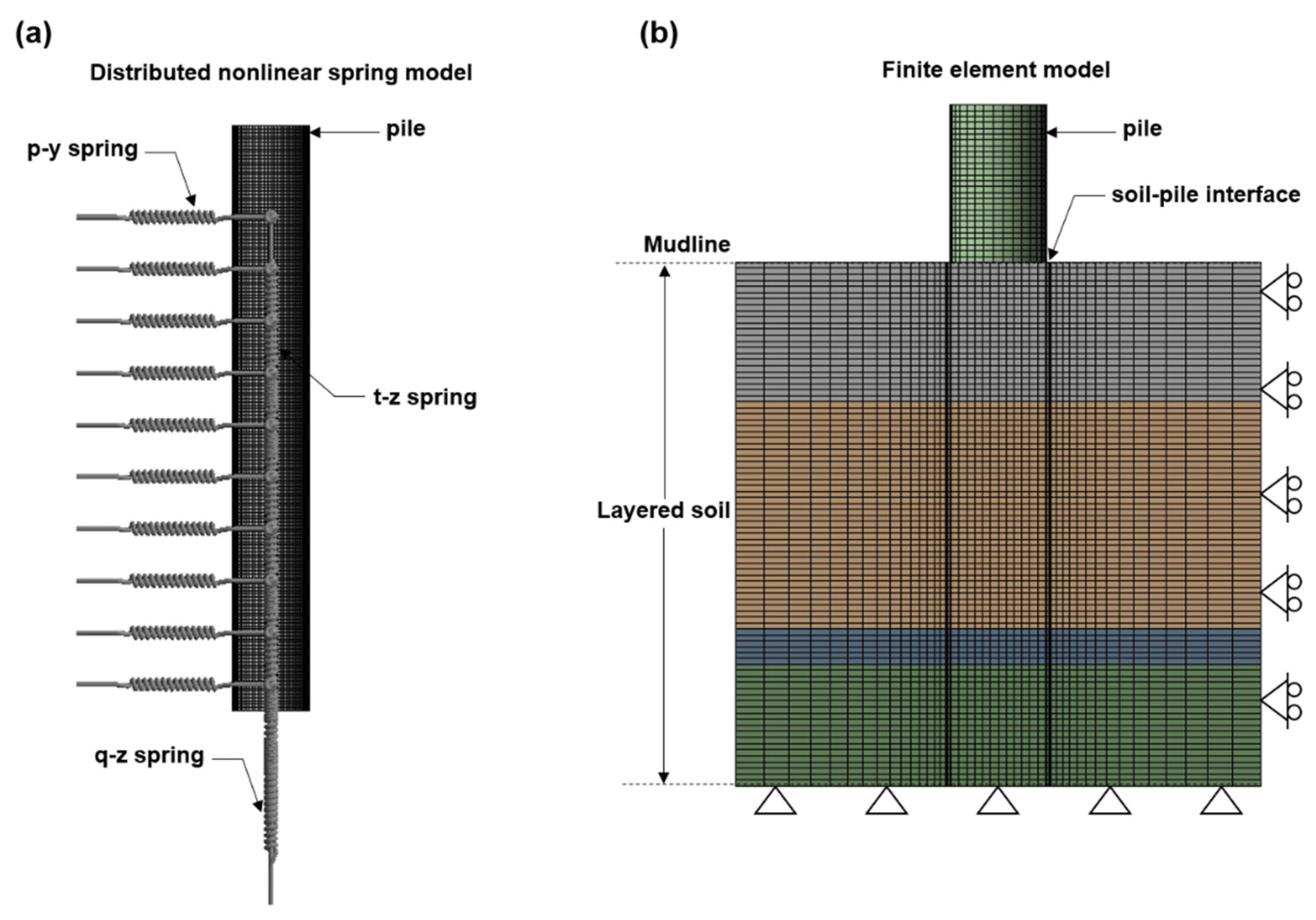
2.3. Three-Dimensional Soil-Structure Interaction
3. Finite Element Model
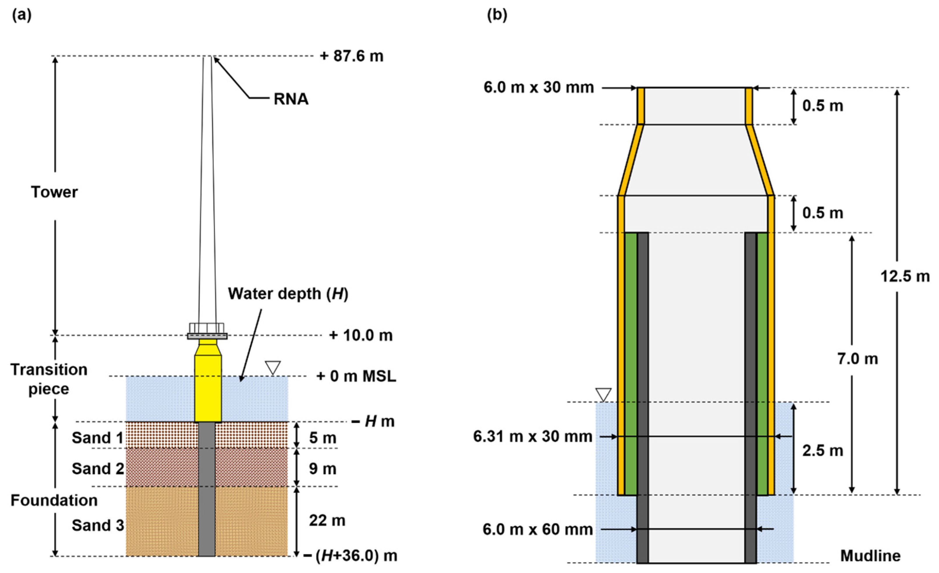
3.1. FE Model for Wind Turbine and Soil Layers
3.2. Verification of FE Models
4. Results and Discussion
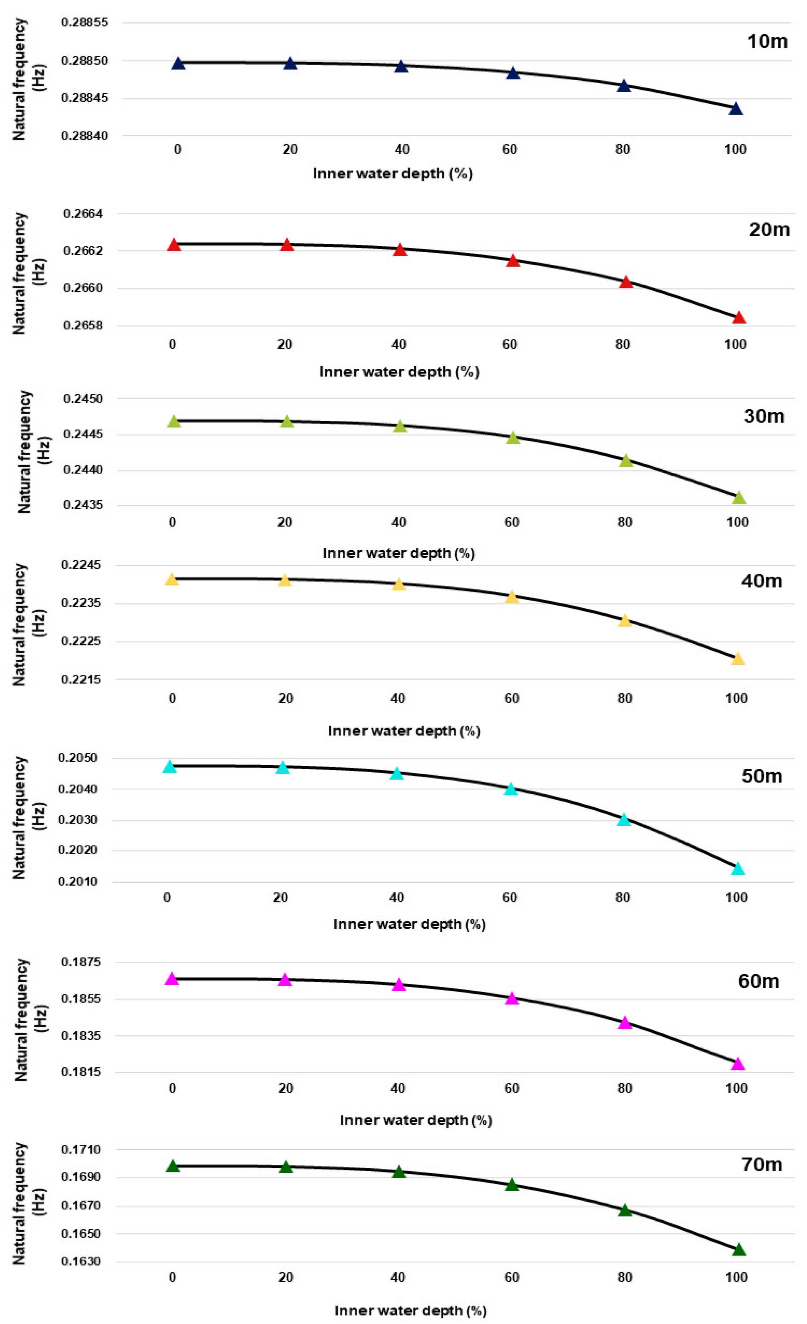
4.1. Impact of Inner Water Level and Water Depth Parameters
4.2. Comparison with Derived Equation for Considering Inner Water
5. Conclusions
Author Contributions
Funding
Institutional Review Board Statement
Informed Consent Statement
Data Availability Statement
Conflicts of Interest
References
- Ellingwood, B.R. Reliability-based condition assessment and LRFD for existing structures. Struct. Saf. 1996, 18, 67–80. [Google Scholar] [CrossRef]
- STANDARD DNV GL ST 0437; Loads and Site Conditions for Wind Turbines. DNV GL: Oslo, Norway, 2016.
- Sánchez, S.; López-Gutiérrez, J.-S.; Negro, V.; Esteban, M.D. Foundations in Offshore Wind Farms: Evolution, Characteristics and Range of Use. Analysis of Main Dimensional Parameters in Monopile Foundations. J. Mar. Sci. Eng. 2019, 7, 441. [Google Scholar] [CrossRef] [Green Version]
- Europe, W. Offshore Wind in Europe: Key Trends and Statistics. 2018. Available online: https://windeurope.org/about-wind/statistics/offshore/european-offshore-wind-industry-key-trends-statistics-2018/ (accessed on 14 May 2022).
- DNVGL-ST-0126; Support Structures for Wind Turbines. DNV GL: Oslo, Norway, 2016.
- Devriendt, C.; Weijtjens, W.; El-Kafafy, M.; De Sitter, G. Monitoring resonant frequencies and damping values of an offshore wind turbine in parked conditions. IET Renew. Power Gener. 2014, 8, 433–441. [Google Scholar] [CrossRef] [Green Version]
- Sunday, K.; Brennan, F. A review of offshore wind monopiles structural design achievements and challenges. Ocean Eng. 2021, 235, 109409. [Google Scholar] [CrossRef]
- Arany, L.; Bhattacharya, S.; Macdonald, J.H.; Hogan, S.J. Closed form solution of Eigen frequency of monopile supported offshore wind turbines in deeper waters incorporating stiffness of substructure and SSI. Soil Dyn. Earthq. Eng. 2016, 83, 18–32. [Google Scholar] [CrossRef] [Green Version]
- Hilbert, L.; Black, A.; Andersen, F.; Mathiesen, T. Inspection and monitoring of corrosion inside monopile foundations for offshore wind turbines. Eur. Corros. Congr. 2011, 3, 2187–2201. [Google Scholar]
- Damgaard, M.; Andersen, J.K. Natural frequency and damping estimation of an offshore wind turbine structure. In Proceedings of the the Twenty-Second International Offshore and Polar Engineering Conference, Rhodes, Greece, 17–22 June 2012. [Google Scholar]
- Kallehave, D.; Thilsted, C.L.; Liingaard, M. Modification of the API py formulation of initial stiffness of sand. In Proceedings of the Offshore Site Investigation and Geotechnics: Integrated Technologies-Present and Future, London, UK, 12–14 September 2012. [Google Scholar]
- Kühn, M. Soft or stiff-a fundamental question in the design of offshore wind energy converters. In Proceedings of the European Wind Energy Conference, Dublin Castle, Ireland, 6–9 October 1997; pp. 575–578. [Google Scholar]
- Lowe, J. Hornsea Met Mast-A Demonstration of the ‘Twisted Jacket’Design. In Proceedings of the Future Offshore Wind Turbine Foundation Conference, Bremen, Germany, 2 February 2012. [Google Scholar]
- Zaaijer, M. Design Methods for Offshore Wind Turbines at Exposed Sites (OWTES)—Sensitivity Analysis for Foundations of Offshore Wind Turbines; Garrad Hassan: Delft, The Netherlands, 2002. [Google Scholar]
- Zania, V. Natural vibration frequency and damping of slender structures founded on monopiles. Soil Dyn. Earthq. Eng. 2014, 59, 8–20. [Google Scholar] [CrossRef]
- Prendergast, L.J.; Gavin, K.; Doherty, P. An investigation into the effect of scour on the natural frequency of an offshore wind turbine. Ocean Eng. 2015, 101, 1–11. [Google Scholar] [CrossRef] [Green Version]
- Yi, J.-H.; Kim, S.-B.; Yoon, G.-L.; Andersen, L.V. Natural frequency of bottom-fixed offshore wind turbines considering pile-soil-interaction with material uncertainties and scouring depth. Wind. Struct. 2015, 21, 625–639. [Google Scholar] [CrossRef]
- van der Tempel, J.; Molenaar, D.-P. Wind turbine structural dynamics—A review of the principles for modern power generation, onshore and offshore. Wind Eng. 2002, 26, 211–222. [Google Scholar] [CrossRef]
- Adhikari, S.; Bhattacharya, S. Dynamic analysis of wind turbine towers on flexible foundations. Shock Vib. 2012, 19, 37–56. [Google Scholar] [CrossRef]
- Ko, Y.-Y. A simplified structural model for monopile-supported offshore wind turbines with tapered towers. Renew. Energy 2020, 156, 777–790. [Google Scholar] [CrossRef]
- Wang, P.; Xu, Y.; Zhang, X.; Xi, R.; Du, X. A substructure method for seismic responses of offshore wind turbine considering nonlinear pile-soil dynamic interaction. Soil Dyn. Earthq. Eng. 2021, 144, 106684. [Google Scholar] [CrossRef]
- Darvishi-Alamouti, S.; Bahaari, M.-R.; Moradi, M. Natural frequency of offshore wind turbines on rigid and flexible monopiles in cohesionless soils with linear stiffness distribution. Appl. Ocean. Res. 2017, 68, 91–102. [Google Scholar] [CrossRef]
- Kramer, S.L. Geotechnical Earthquake Engineering; Pearson Education India: Nodia, India, 1996. [Google Scholar]
- Jhung, M.J.; Kang, S.-S. Fluid effect on the modal characteristics of a square tank. Nucl. Eng. Technol. 2019, 51, 1117–1131. [Google Scholar] [CrossRef]
- Morand, H.J.-P.; Ohayon, R. Fluid Structure Interaction. Wiley & Sons. 1995. Available online: https://onlinelibrary.wiley.com/doi/10.1002/zamm.19960760705 (accessed on 14 May 2022).
- Benra, F.-K.; Dohmen, H.J.; Pei, J.; Schuster, S.; Wan, B. A comparison of one-way and two-way coupling methods for numerical analysis of fluid-structure interactions. J. Appl. Math. 2011, 2011, 853560. [Google Scholar] [CrossRef]
- Gutknecht, M.H. The unsymmetric Lanczos algorithms and their relations to P ade approximation, continued fractions and the QD algorithm. In Proceedings of the Copper Mountain Conference on Iterative Methods, Copper Mountain, CO, USA, 9–13 April 1990. [Google Scholar]
- Rajakumar, C.; Rogers, C. The Lanczos algorithm applied to unsymmetric generalized eigenvalue problem. Int. J. Numer. Methods Eng. 1991, 32, 1009–1026. [Google Scholar] [CrossRef]
- Bankar, S.S. Vibration and Acoustic Analysis of Laminated Composite Plate. Ph.D. Thesis, National Institute of Technology Rourkela, Odisha, India, May 2015. [Google Scholar]
- American Petroleum Institute. Planning, Designing, and Constructing Fixed Offshore Platforms—Working Stress Design; American Petroleum Institute: Washington, DC, USA, 2014. [Google Scholar]
- DNVGL-RP-C212; Offshore Soil Mechanics and Geotechnical Engineering. DNV GL: Høvik, Norway, 2017.
- Abdullahi, A.; Wang, Y.; Bhattacharya, S. Comparative Modal Analysis of Monopile and Jacket Supported Offshore Wind Turbines including Soil-Structure Interaction. Int. J. Struct. Stab. Dyn. 2020, 20, 2042016. [Google Scholar] [CrossRef]
- Jalbi, S.; Shadlou, M.; Bhattacharya, S. Practical method to estimate foundation stiffness for design of offshore wind turbines. In Wind Energy Engineering; Elsevier: Amsterdam, The Netherlands, 2017; pp. 329–352. [Google Scholar]
- Abhinav, K.; Saha, N. Dynamic analysis of an offshore wind turbine including soil effects. Procedia Eng. 2015, 116, 32–39. [Google Scholar] [CrossRef] [Green Version]
- Jonkman, J.; Butterfield, S.; Musial, W.; Scott, G. Definition of a 5-MW Reference Wind Turbine for Offshore System Development; National Renewable Energy Lab. (NREL): Golden, CO, USA, 2009.
- Gentils, T.; Wang, L.; Kolios, A. Integrated structural optimisation of offshore wind turbine support structures based on finite element analysis and genetic algorithm. Appl. Energy 2017, 199, 187–204. [Google Scholar] [CrossRef] [Green Version]
- Shi, W.; Park, H.-C.; Baek, J.-H.; Kim, C.-W.; Kim, Y.-C.; Shin, H.-K. Study on the marine growth effect on the dynamic response of offshore wind turbines. Int. J. Precis. Eng. Manuf. 2012, 13, 1167–1176. [Google Scholar] [CrossRef]
- Jung, S.; Kim, S.-R.; Patil, A. Effect of monopile foundation modeling on the structural response of a 5-MW offshore wind turbine tower. Ocean Eng. 2015, 109, 479–488. [Google Scholar] [CrossRef] [Green Version]
- ANSYS Inc. Contact Technology Guide Release 12.1. 2009. Available online: https://www.cae.tntech.edu (accessed on 14 May 2022).
- Özer, H.; Öz, Ö. Three dimensional finite element analysis of bi-adhesively bonded double lap joint. Int. J. Adhes. Adhes. 2012, 37, 50–55. [Google Scholar] [CrossRef]
- Lanoue, F.; Vadean, A.; Sanschagrin, B. Finite element analysis and contact modelling considerations of interference fits for fretting fatigue strength calculations. Simul. Model. Pract. Theory 2009, 17, 1587–1602. [Google Scholar] [CrossRef]
- Daneshi, M. Numerical investigation of the fluid flow around and past a circular cylinder by ANSYS simulation. Int. J. Adv. Sci. Technol. 2016, 92, 49–58. [Google Scholar] [CrossRef]
- Tran, T.; Kim, D.; Song, J. Computational fluid dynamic analysis of a floating offshore wind turbine experiencing platform pitching motion. Energies 2014, 7, 5011–5026. [Google Scholar] [CrossRef]
- Kolios, A.; Wang, L.; Mehmanparast, A.; Brennan, F. Determination of stress concentration factors in offshore wind welded structures through a hybrid experimental and numerical approach. Ocean Eng. 2019, 178, 38–47. [Google Scholar] [CrossRef] [Green Version]
- Jonkman, J.; Musial, W. Offshore Code Comparison Collaboration (OC3) for IEA Wind Task 23 Offshore Wind Technology and Deployment; National Renewable Energy Lab. (NREL): Golden, CO, USA, 2010.
- Carswell, W. Probabilistic Analysis of Offshore Wind Turbine Soil-Structure Interaction. Master’s Thesis, University of Massachusetts Amherst, Amherst, MA, USA, 2012. [Google Scholar]


| Contents | Value |
|---|---|
| Length of tower | 87.6 m |
| Total mass of tower | 347,460 kg |
| Outer diameter of tower top | 3.87 m |
| Thickness of tower top | 0.019 m |
| Outer diameter of tower bottom | 6.0 m |
| Thickness of tower bottom | 0.027 m |
| Total weight of RNA | 350,000 kg |
| CM height from tower top of RNA | 1.817 m |
| Material | Young’s Modulus (GPa) | Poisson’s Ratio (-) | Density (kg/m3) |
|---|---|---|---|
| Steel | 210 | 0.38 | 8500 |
| Grout | 70 | 0.19 | 2740 |
| Material | Depth (m) | (kN/m3) | (kPa) | (Degree) | (-) | (MPa) | Dilation Angle (Degree) |
|---|---|---|---|---|---|---|---|
| Sand 1 | 0.0–5.0 | 10.0 | 0.05 | 33.0 | 0.3 | 30.0 | 3.0 |
| Sand 2 | 5.0–14.0 | 10.0 | 0.05 | 35.0 | 0.3 | 35.0 | 5.0 |
| Sand 3 | 14.0–36.0 | 10.0 | 0.05 | 38.5 | 0.3 | 47.0 | 8.5 |
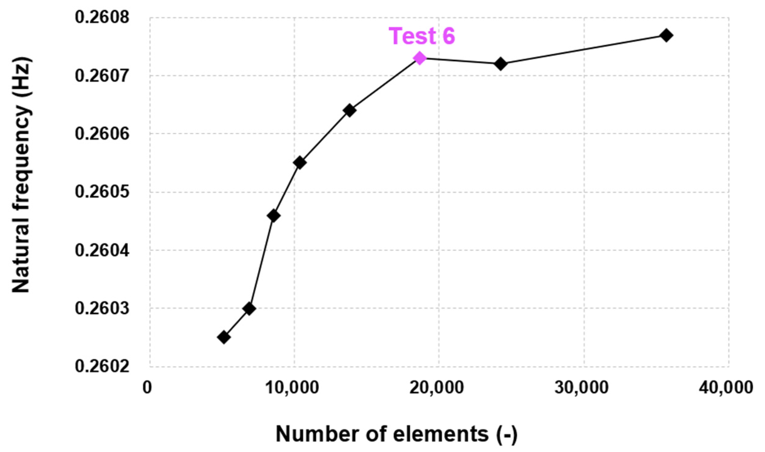
| Test No. | Number of Elements (-) | Natural Frequency (Hz) | Difference (%) |
|---|---|---|---|
| 1 | 5148 | 0.26025 | - |
| 2 | 6894 | 0.26030 | 0.0192 |
| 3 | 8580 | 0.26046 | 0.0615 |
| 4 | 10,386 | 0.26055 | 0.0346 |
| 5 | 13,788 | 0.26064 | 0.0345 |
| 6 | 18,673 | 0.26073 | 0.0345 |
| 7 | 24,275 | 0.26072 | −0.0038 |
| 8 | 35,700 | 0.26077 | 0.0192 |
| Support Conditions | Method | 1st Tower Fore-Aft (Hz) | 1st Tower Side-to-Side (Hz) | Relative Difference (%) | |
|---|---|---|---|---|---|
| 1st Tower Fore-Aft | 1st Tower Side-to-Side | ||||
| Rigid base | (present) | 0.3245 | 0.3250 | - | - |
| FAST [35] | 0.3240 | 0.3120 | 0.14 | 4.00 | |
| ADAMS [35] | 0.3195 | 0.3164 | 1.54 | 2.65 | |
| [20] | 0.3123 | 0.3123 | 3.76 | 3.91 | |
| [20] | 0.3132 | 0.3132 | 3.48 | 3.63 | |
| Fixed soil | (present) | 0.2763 | 0.2766 | - | - |
| [36] | 0.2760 | 0.2780 | 0.09 | −0.51 | |
| [45] | 0.2770 | 0.2780 | −0.27 | −0.51 | |
| Flexible soil | (present) | 0.2548 | 0.2550 | - | - |
| [38] | 0.2420 | 0.2410 | 5.02 | 5.49 | |
| [36] | 0.2450 | 0.2480 | 3.85 | 2.75 | |
| IWL (%) | Depth (m) | ||||||
|---|---|---|---|---|---|---|---|
| 10 | 20 | 30 | 40 | 50 | 60 | 70 | |
| 0 | D10M0 | D20M0 | D30M0 | D40M0 | D50M0 | D60M0 | D70M0 |
| 20 | D10M20 | D20M20 | D30M20 | D40M20 | D50M20 | D60M20 | D70M20 |
| 40 | D10M40 | D20M40 | D30M40 | D40M40 | D50M40 | D60M40 | D70M40 |
| 60 | D10M60 | D20M60 | D30M60 | D40M60 | D50M60 | D60M60 | D70M60 |
| 80 | D10M80 | D20M80 | D30M80 | D40M80 | D50M80 | D60M80 | D70M80 |
| 100 | D10M100 | D20M100 | D30M100 | D40M100 | D50M100 | D60M100 | D70M100 |
| IWL (%) | Depth (m) | ||||||
|---|---|---|---|---|---|---|---|
| 10 | 20 | 30 | 40 | 50 | 60 | 70 | |
| 0 | 0.27984 | 0.25591 | 0.23333 | 0.21222 | 0.19257 | 0.17441 | 0.15775 |
| 20 | 0.27983 | 0.25590 | 0.23331 | 0.21220 | 0.19254 | 0.17438 | 0.15771 |
| 40 | 0.27982 | 0.25587 | 0.23326 | 0.21212 | 0.19242 | 0.17421 | 0.15751 |
| 60 | 0.27981 | 0.25582 | 0.23314 | 0.21189 | 0.19205 | 0.17369 | 0.15683 |
| 80 | 0.27979 | 0.25573 | 0.23289 | 0.21139 | 0.19121 | 0.17245 | 0.15518 |
| 100 | 0.27976 | 0.25558 | 0.23246 | 0.21046 | 0.18959 | 0.17003 | 0.15196 |
| IWL (%) | Depth (m) | ||||||
|---|---|---|---|---|---|---|---|
| 10 | 20 | 30 | 40 | 50 | 60 | 70 | |
| 0 | 0.28018 | 0.25617 | 0.23352 | 0.21237 | 0.19267 | 0.17448 | 0.15780 |
| 20 | 0.28017 | 0.25615 | 0.23350 | 0.21234 | 0.19264 | 0.17445 | 0.15777 |
| 40 | 0.28016 | 0.25613 | 0.23345 | 0.21226 | 0.19252 | 0.17429 | 0.15756 |
| 60 | 0.28015 | 0.25608 | 0.23333 | 0.21203 | 0.19215 | 0.17376 | 0.15688 |
| 80 | 0.28013 | 0.25598 | 0.23308 | 0.21153 | 0.19131 | 0.17253 | 0.15523 |
| 100 | 0.28010 | 0.25584 | 0.23265 | 0.21059 | 0.18969 | 0.17010 | 0.15201 |
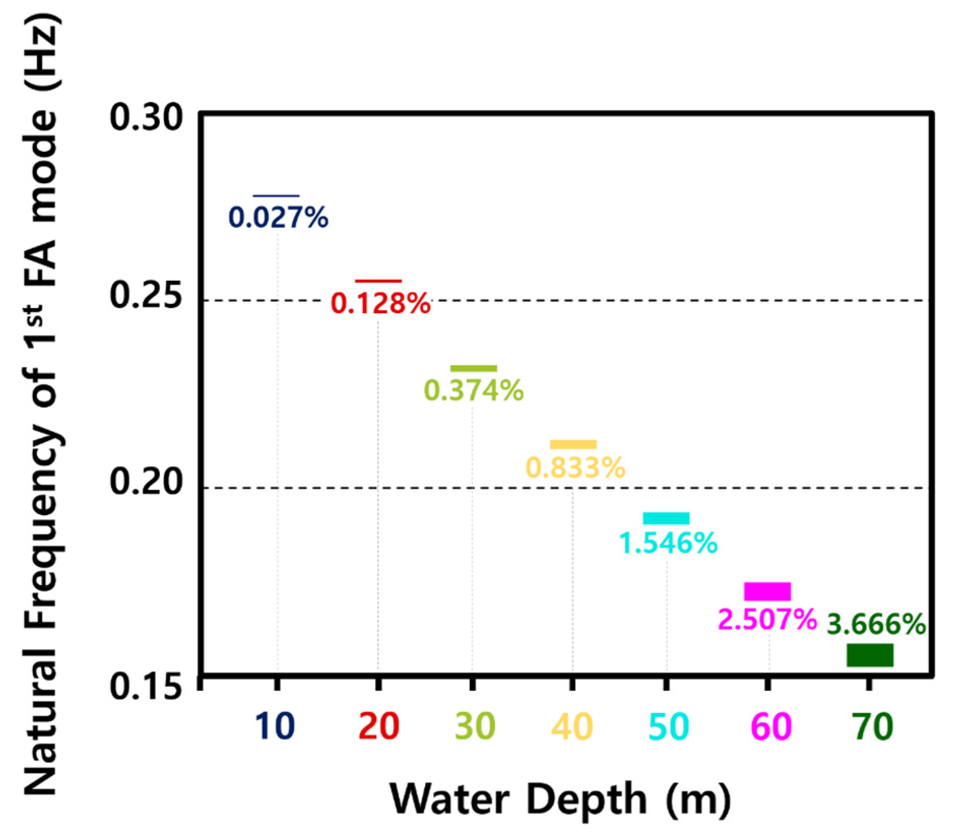
| Item | Water Depth | 10 m | 20 m | 30 m | 40 m | 50 m | 60 m | 70 m |
|---|---|---|---|---|---|---|---|---|
| A | 0.2885 | 0.2662 | 0.2447 | 0.2241 | 0.2048 | 0.1866 | 0.1699 | |
| B | 0.2884 | 0.2658 | 0.2436 | 0.2221 | 0.2014 | 0.1820 | 0.1639 | |
| C | Results | 0.2801 | 0.2558 | 0.2326 | 0.2106 | 0.1897 | 0.1701 | 0.1520 |
| Difference between A and C (%) | 2.90 | 3.90 | 4.93 | 6.05 | 7.36 | 8.86 | 10.51 | |
| Difference between B and C (%) | 2.89 | 3.77 | 4.51 | 5.17 | 5.84 | 6.54 | 7.28 |
Publisher’s Note: MDPI stays neutral with regard to jurisdictional claims in published maps and institutional affiliations. |
© 2022 by the authors. Licensee MDPI, Basel, Switzerland. This article is an open access article distributed under the terms and conditions of the Creative Commons Attribution (CC BY) license (https://creativecommons.org/licenses/by/4.0/).
Share and Cite
You, Y.-S.; Song, K.-Y.; Sun, M.-Y. Variable Natural Frequency Damper for Minimizing Response of Offshore Wind Turbine: Principle Verification through Analysis of Controllable Natural Frequencies. J. Mar. Sci. Eng. 2022, 10, 983. https://doi.org/10.3390/jmse10070983
You Y-S, Song K-Y, Sun M-Y. Variable Natural Frequency Damper for Minimizing Response of Offshore Wind Turbine: Principle Verification through Analysis of Controllable Natural Frequencies. Journal of Marine Science and Engineering. 2022; 10(7):983. https://doi.org/10.3390/jmse10070983
Chicago/Turabian StyleYou, Young-Suk, Ka-Young Song, and Min-Young Sun. 2022. "Variable Natural Frequency Damper for Minimizing Response of Offshore Wind Turbine: Principle Verification through Analysis of Controllable Natural Frequencies" Journal of Marine Science and Engineering 10, no. 7: 983. https://doi.org/10.3390/jmse10070983
APA StyleYou, Y.-S., Song, K.-Y., & Sun, M.-Y. (2022). Variable Natural Frequency Damper for Minimizing Response of Offshore Wind Turbine: Principle Verification through Analysis of Controllable Natural Frequencies. Journal of Marine Science and Engineering, 10(7), 983. https://doi.org/10.3390/jmse10070983