
Time-Optimal Path Planning of a Hybrid Autonomous Underwater Vehicle Based on Ocean Current Neural Point Grid


Abstract
:1. Introduction
1.1. Background
1.2. Related Work
1.3. Article Structure
- In the paper, two path planning algorithms are run in different grid maps to plan time-optimal paths. The two algorithms are also compared in terms of program running time. In fact, a suitable path planning method can not only improve the efficiency of the path search, but it can also obtain time-optimal solution.
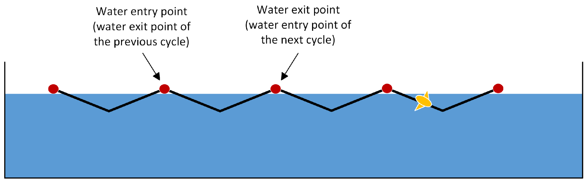
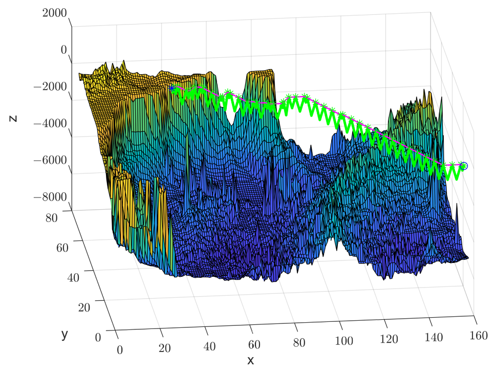
- The path is numerically separated to produce a series of waypoints related to the underwater motion of the HAUV in glider mode. The article simulates the motion trajectory of the HAUV based on the waypoints.
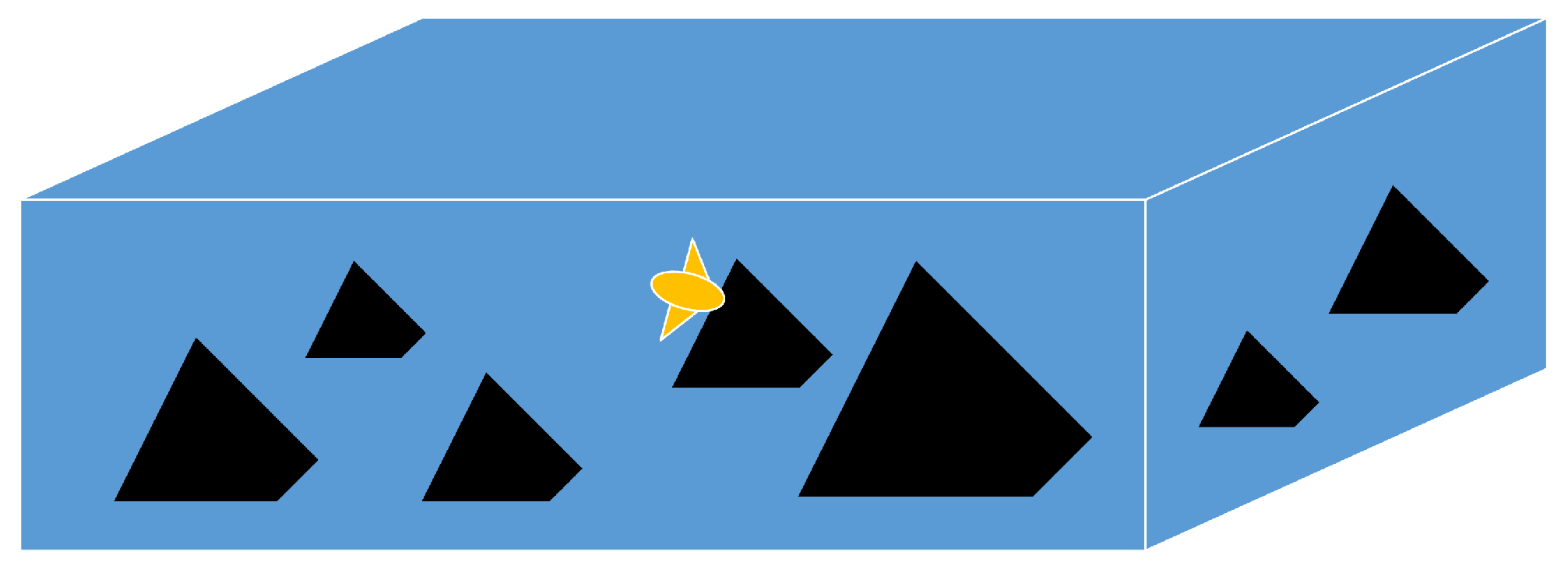
- The influence of the riverbed on the HAUV is considered when waypoints are planned, so that the HAUV is capable of avoiding hitting the riverbed while traveling.
2. Problem
2.1. HAUV Overview
2.2. Path Planning
2.2.1. Path Planning under Ocean Currents
2.2.2. HAUV Travel Planning
3. Method
3.1. Global Path Planning
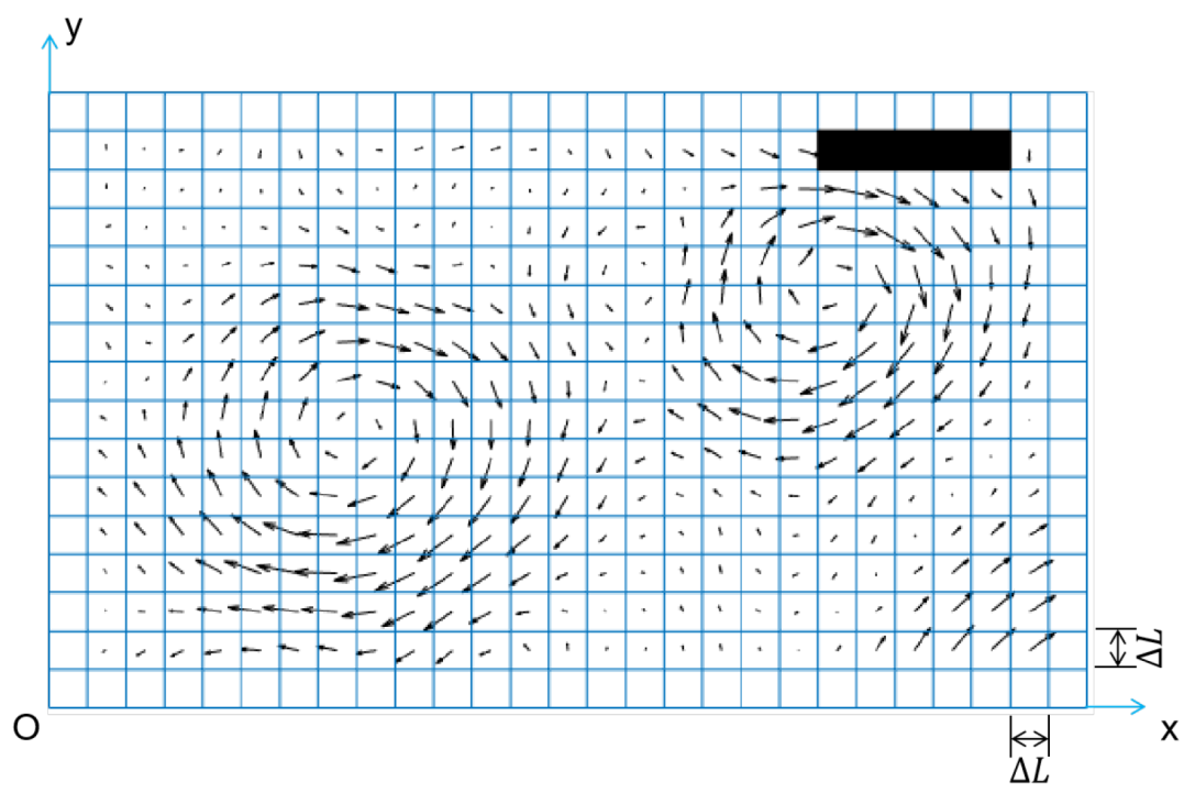
3.1.1. The Grid Map
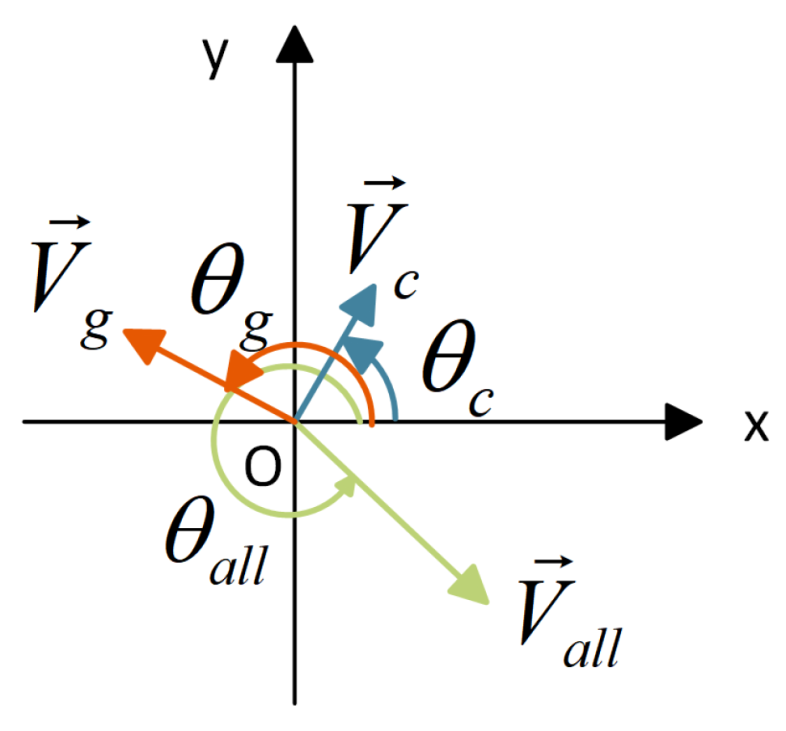
3.1.2. Velocity Modeling
3.1.3. The Improved A* Algorithm
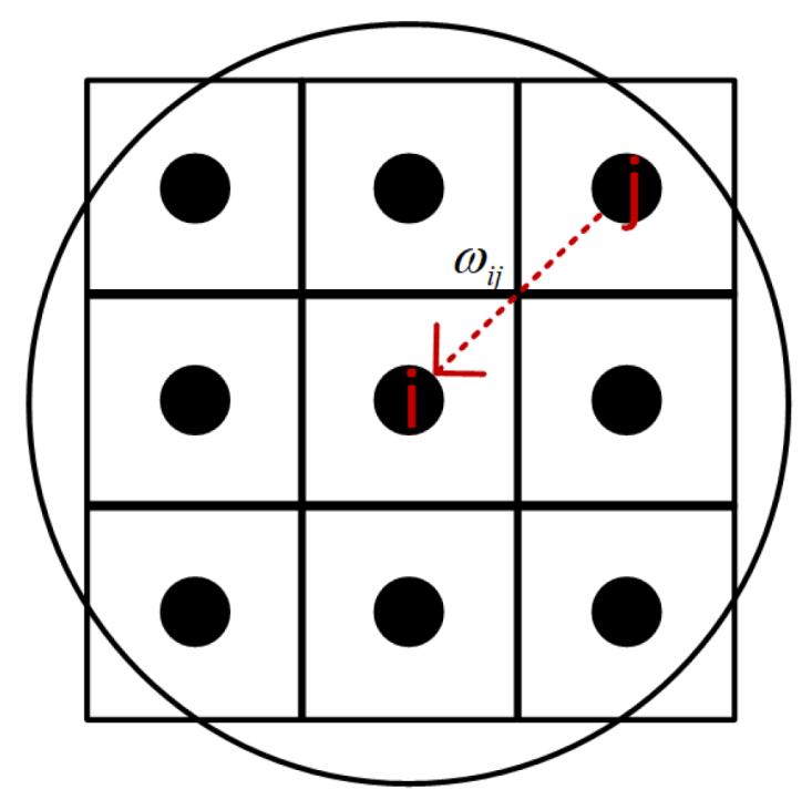
3.1.4. Neural Network Model
3.2. HAUV Travel Planning
4. Simulation
4.1. Data Description
4.2. HAUV Description
4.3. Simulation Results
4.3.1. Global Path Planning
- 1.
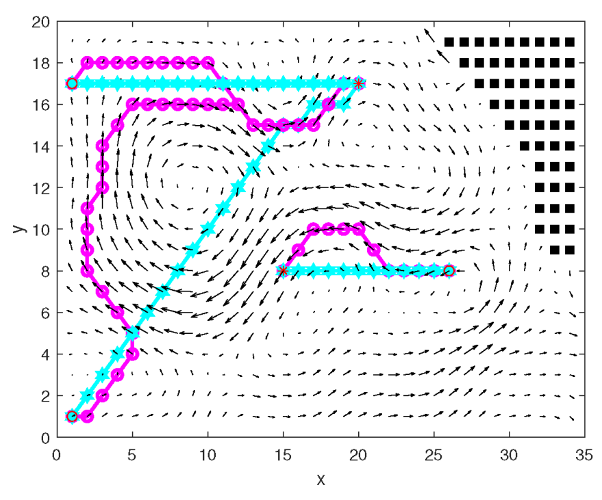
- Comparison of traditional A* algorithm and improved A* algorithm
- 2.
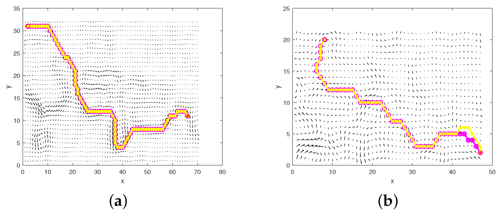
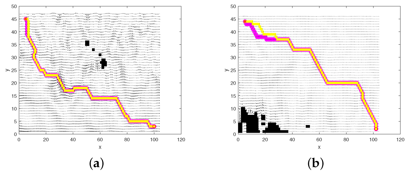
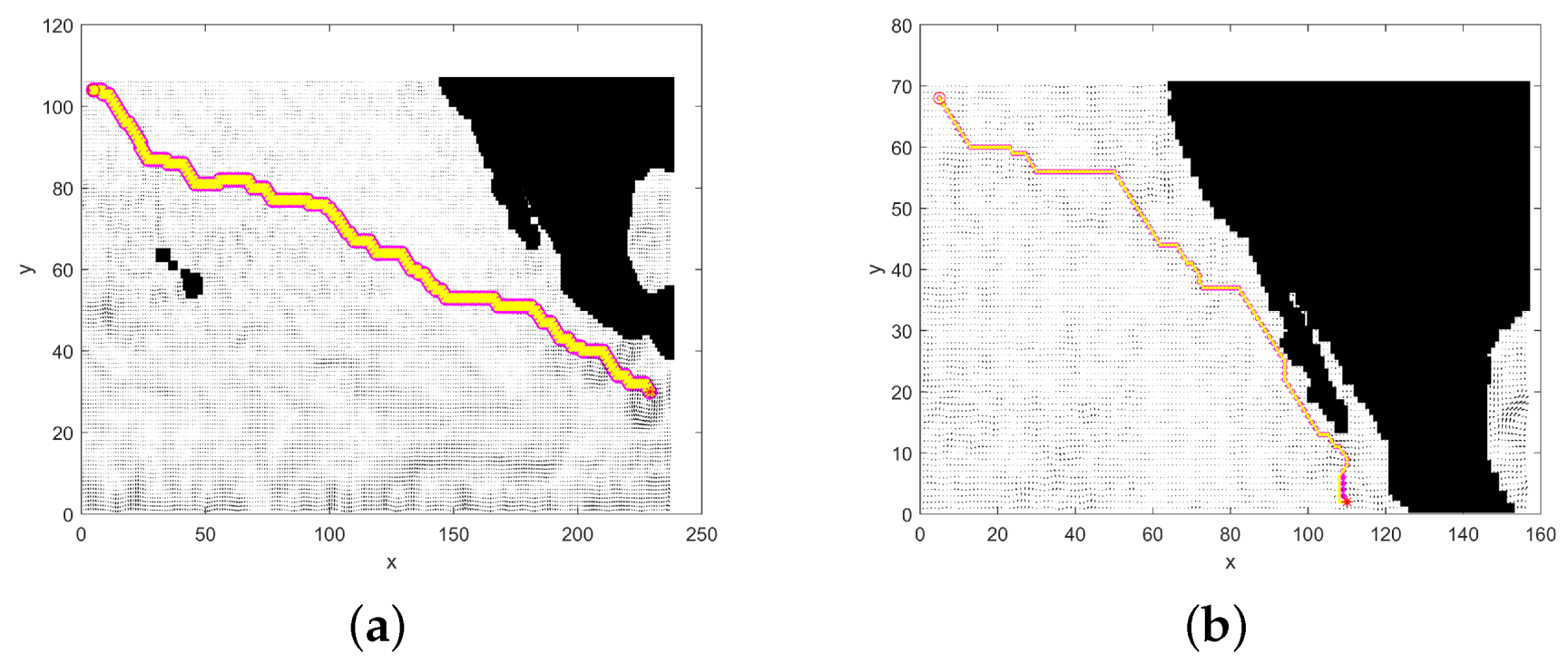
- Paths generated by the improved A* algorithm and neural network model
- 3.
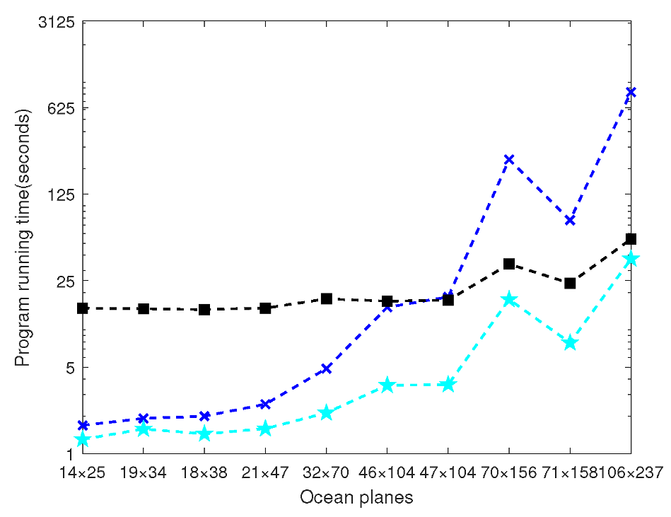
- Comparison of working time
- 4.
- Advantages
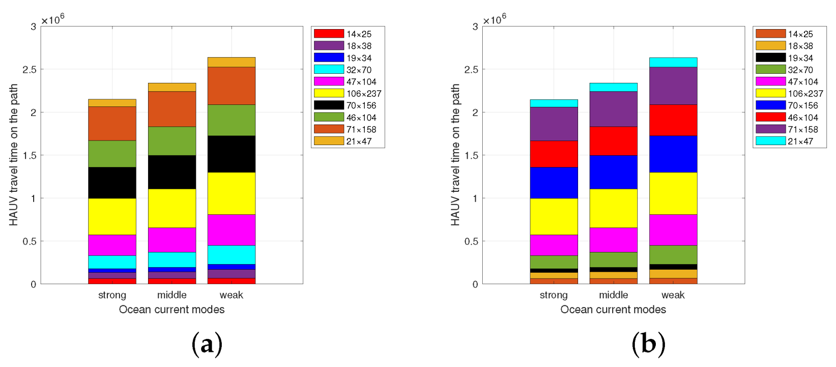
4.3.2. HAUV Travel Planning
5. Conclusions
Author Contributions
Funding
Institutional Review Board Statement
Informed Consent Statement
Data Availability Statement
Conflicts of Interest
References
- Wang, M.; Sun, F.; Gu, S. Application of Markov Decision Process in Delivery Robot Path Planning System. Int. Core J. Eng. 2021, 7, 485–491. [Google Scholar]
- Khan, M.T.R.; Muhammad Saad, M.; Ru, Y.; Seo, J.; Kim, D. Aspects of unmanned aerial vehicles path planning: Overview and applications. Int. J. Commun. Syst. 2021, 34, e4827. [Google Scholar] [CrossRef]
- Asmaa, I.; Khalid, B. UAV Path Planning for Civil Applications. Int. J. Adv. Comput. Sci. Appl. 2019, 10, 635. [Google Scholar] [CrossRef]
- Akshya, J.; Priyadarsini, P. Graph-based path planning for intelligent UAVs in area coverage applications. J. Intell. Fuzzy Syst. 2020, 39, 8191–8203. [Google Scholar] [CrossRef]
- Shi, Y.; Zhang, L.; Dong, S. Path Planning of Anti-ship Missile based on Voronoi Diagram and Binary Tree Algorithm. Def. Sci. J. 2019, 69, 369–377. [Google Scholar] [CrossRef]
- Yang, X.; Yan, J.; Hua, C.; Guan, X. Trajectory tracking control of autonomous underwater vehicle with unknown parameters and external disturbances. IEEE Trans. Syst. Man Cybern. Syst. 2019, 51, 1054–1063. [Google Scholar] [CrossRef]
- Kavraki, L.E.; Svestka, P.; Latombe, J.C.; Overmars, M.H. Probabilistic roadmaps for path planning in high-dimensional configuration spaces. IEEE Trans. Robot. Autom. 1996, 12, 566–580. [Google Scholar] [CrossRef] [Green Version]
- Martınez-Alfaro, H.; Gomez-Garcıa, S. Mobile robot path planning and tracking using simulated annealing and fuzzy logic control. Expert Syst. Appl. 1998, 15, 421–429. [Google Scholar] [CrossRef]
- Orozco-Rosas, U.; Montiel, O.; Sepúlveda, R. Mobile robot path planning using membrane evolutionary artificial potential field. Appl. Soft Comput. 2019, 77, 236–251. [Google Scholar] [CrossRef]
- Yu, Z.Z.; Yan, J.H.; Zhao, J.; Chen, Z.F.; Zhu, Y.H. Mobile robot path planning based on improved artificial potential field method. Harbin Gongye Daxue Xuebao (J. Harbin Inst. Technol.) 2011, 43, 50–55. [Google Scholar]
- Xiong, X.; Min, H.; Yu, Y.; Wang, P. Application improvement of A* algorithm in intelligent vehicle trajectory planning. Math. Biosci. Eng. 2021, 18, 1–21. [Google Scholar] [CrossRef] [PubMed]
- Li, X. Path planning of intelligent mobile robot based on Dijkstra algorithm. In Proceedings of the Journal of Physics: Conference Series; IOP Publishing: Bristol, UK, 2021. [Google Scholar]
- Lyu, D.; Chen, Z.; Cai, Z.; Piao, S. Robot path planning by leveraging the graph-encoded Floyd algorithm. Future Gener. Comput. Syst. 2021, 122, 204–208. [Google Scholar] [CrossRef]
- Lv, Y. Application of Artificial Intelligence Combined with Neural Network in the Research of Mobile Robot Path Planning. J. Phys. Conf. Ser. 2020, 1648, 032145. [Google Scholar] [CrossRef]
- Hasan, A.H.; Sadiq, A.T. Robot path planning based on hybrid improved D* with particle swarm optimization algorithms in dynamic environment. J. Comput. Theor. Nanosci. 2019, 16, 1062–1073. [Google Scholar] [CrossRef]
- Wangsheng, F.; Chong, W.; Ruhua, Z. Application of simulated annealing particle swarm optimization in complex three-dimensional path planning. In Proceedings of the Journal of Physics: Conference Series; IOP Publishing: Bristol, UK, 2021. [Google Scholar]
- Zhang, B.; Wang, Y.C.; Zhang, X.L. Mobile Robot Path Planning Based on Ant Colony Optimization. Laser J. 2016, 687–691, 706–709. [Google Scholar] [CrossRef]
- Lu, J.; Liang, Z.; Li, X.; Zhu, Z.; Wei, B.; Fang, F. The Application of Adaptive Ant-colony A* Hybrid Algorithm Based on Objective Evaluation Factor in RoboCup Rescue Simulation Dynamic Path Planning. In Proceedings of the IOP Conference Series: Materials Science and Engineering; IOP Publishing: Bristol, UK, 2019. [Google Scholar]
- Lamini, C.; Benhlima, S.; Elbekri, A. Genetic algorithm based approach for autonomous mobile robot path planning. Procedia Comput. Sci. 2018, 127, 180–189. [Google Scholar] [CrossRef]
- Yang, S.X.; Luo, C. A neural network approach to complete coverage path planning. IEEE Trans. Syst. Man. Cybern. Part B (Cybern.) 2004, 34, 718–724. [Google Scholar] [CrossRef]
- Yi, X.; Zhu, A.; Yang, S.X.; Luo, C. A bio-inspired approach to task assignment of swarm robots in 3-D dynamic environments. IEEE Trans. Cybern. 2016, 47, 974–983. [Google Scholar] [CrossRef]
- Li, H.; Yang, S.X.; Seto, M.L. Neural-network-based path planning for a multirobot system with moving obstacles. IEEE Trans. Syst. Man. Cybern. Part C (Appl. Rev.) 2009, 39, 410–419. [Google Scholar] [CrossRef]
- MahmoudZadeh, S.; Powers, D.; Yazdani, A.M.; Sammut, K.; Atyabi, A. Efficient AUV path planning in time-variant underwater environment using differential evolution algorithm. J. Mar. Sci. Appl. 2018, 17, 585–591. [Google Scholar] [CrossRef]
- Huang, H.; Jin, C. A Novel Particle Swarm Optimization Algorithm Based on Reinforcement Learning Mechanism for AUV Path Planning. Complexity 2021, 2021, 8993173. [Google Scholar] [CrossRef]
- Yao, P.; Zhao, S. Three-dimensional path planning for AUV based on interfered fluid dynamical system under ocean current (June 2018). IEEE Access 2018, 6, 42904–42916. [Google Scholar] [CrossRef]
- Yao, X.; Wang, F.; Yuan, C.; Wang, J.; Wang, X. Path planning for autonomous underwater vehicles based on interval optimization in uncertain flow fields. Ocean. Eng. 2021, 234, 108675. [Google Scholar] [CrossRef]
- Cao, X.; Sun, C.Y.; Chen, M.Z. Path planning for autonomous underwater vehicle in time-varying current. IET Intell. Transp. Syst. 2019, 13, 1265–1271. [Google Scholar] [CrossRef]
- Alvarez, A.; Caiti, A.; Onken, R. Evolutionary path planning for autonomous underwater vehicles in a variable ocean. IEEE J. Ocean. Eng. 2004, 29, 418–429. [Google Scholar] [CrossRef]
- Zeng, Z.; Zhou, H.; Lian, L. Exploiting ocean energy for improved AUV persistent presence: Path planning based on spatiotemporal current forecasts. J. Mar. Sci. Technol. 2020, 25, 26–47. [Google Scholar] [CrossRef]
- Shah, B.C.; Gupta, S.K. Speeding up A* search on visibility graphs defined over quadtrees to enable long distance path planning for unmanned surface vehicles. In Proceedings of the Twenty-Sixth International Conference on Automated Planning and Scheduling, London, UK, 12–17 June 2016. [Google Scholar]
- Lin, C.; Han, G.; Du, J.; Bi, Y.; Shu, L.; Fan, K. A Path Planning Scheme for AUV Flock-Based Internet-of-Underwater-Things Systems to Enable Transparent and Smart Ocean. IEEE Internet Things J. 2020, 7, 9760–9772. [Google Scholar] [CrossRef]
- Wang, N.; Xu, H. Dynamics-constrained global-local hybrid path planning of an autonomous surface vehicle. IEEE Trans. Veh. Technol. 2020, 69, 6928–6942. [Google Scholar] [CrossRef]
- Zamuda, A.; Sosa, J.D.H. Differential evolution and underwater glider path planning applied to the short-term opportunistic sampling of dynamic mesoscale ocean structures. Appl. Soft Comput. 2014, 24, 95–108. [Google Scholar] [CrossRef]
- Wang, Z.; Li, G.; Ren, J. Dynamic path planning for unmanned surface vehicle in complex offshore areas based on hybrid algorithm. Comput. Commun. 2021, 166, 49–56. [Google Scholar] [CrossRef]
- Alam, T.; Al Redwan Newaz, A.; Bobadilla, L.; Alsabban, W.H.; Smith, R.N.; Karimoddini, A. Towards energy-aware feedback planning for long-range autonomous underwater vehicles. Front. Robot. AI 2021, 8, 621820. [Google Scholar] [CrossRef] [PubMed]
- Lolla, T.; Ueckermann, M.P.; Yiğit, K.; Haley, P.J.; Lermusiaux, P.F. Path planning in time dependent flow fields using level set methods. In Proceedings of the 2012 IEEE International Conference on Robotics and Automation, Guangzhou, China, 11–14 December 2012; IEEE: Piscataway, NJ, USA, 2012; pp. 166–173. [Google Scholar]
- Kularatne, D.; Bhattacharya, S.; Hsieh, M.A. Time and Energy Optimal Path Planning in General Flows. In Proceedings of the Robotics: Science and Systems, Arbor, MI, USA, 18–22 June 2016; pp. 1–10. [Google Scholar]
- Rao, D.; Williams, S.B. Large-scale path planning for underwater gliders in ocean currents. In Proceedings of the Australasian Conference on Robotics and Automation (ACRA), Sydney, Australia, 2–4 December 2009; Citeseer: Princeton, NJ, USA, 2009; pp. 2–4. [Google Scholar]
- Chen, M.; Zhu, D. Optimal Time-Consuming Path Planning for Autonomous Underwater Vehicles Based on a Dynamic Neural Network Model in Ocean Current Environments. IEEE Trans. Veh. Technol. 2020, 69, 14401–14412. [Google Scholar] [CrossRef]
- Zhu, D.; Zhou, B.; Yang, S.X. A novel algorithm of Multi-AUVs task assignment and path planning based on biologically inspired neural network map. IEEE Trans. Intell. Veh. 2020, 6, 333–342. [Google Scholar] [CrossRef]
- Lim, H.S.; Fan, S.; Chin, C.K.; Chai, S.; Bose, N. Particle swarm optimization algorithms with selective differential evolution for AUV path planning. Int. J. Robot. Autom. 2020, 9, 94–112. [Google Scholar] [CrossRef]
- Wei, D.; Wang, F.; Ma, H. Autonomous path planning of AUV in large-scale complex marine environment based on swarm hyper-heuristic algorithm. Appl. Sci. 2019, 9, 2654. [Google Scholar] [CrossRef] [Green Version]
- Zeng, Z.; Lammas, A.; Sammut, K.; He, F. Optimal path planning based on annular space decomposition for AUVs operating in a variable environment. In Proceedings of the 2012 IEEE/OES Autonomous Underwater Vehicles (AUV), Southampton, UK, 24–27 September 2012; IEEE: Piscataway, NJ, USA, 2012; pp. 1–9. [Google Scholar]
- Jenkins, S.A.; Humphreys, D.E.; Sherman, J.; Osse, J.; Jones, C.; Leonard, N.; Graver, J.; Bachmayer, R.; Clem, T.; Carroll, P.; et al. Underwater Glider System Study; Scripps Institution of Oceanography: San Diego, CA, USA, 2003. [Google Scholar]

| The Route | Time Cost of the Route Established by the Traditional A* Algorithm | Time Cost of the Route Established by the Improved A* Algorithm |
|---|---|---|
| The route from (1,1) to (20,17) | ∞ | 45,973 |
| The route from (26,8) to (15,8) | 16,462 | 13,196 |
| The route from (1,17) to (20,17) | 35,565 | 30,091 |
Publisher’s Note: MDPI stays neutral with regard to jurisdictional claims in published maps and institutional affiliations. |
© 2022 by the authors. Licensee MDPI, Basel, Switzerland. This article is an open access article distributed under the terms and conditions of the Creative Commons Attribution (CC BY) license (https://creativecommons.org/licenses/by/4.0/).
Share and Cite
Hua, C.; Wu, N.; Yuan, H.; Chen, X.; Dong, Y.; Zeng, X. Time-Optimal Path Planning of a Hybrid Autonomous Underwater Vehicle Based on Ocean Current Neural Point Grid. J. Mar. Sci. Eng. 2022, 10, 977. https://doi.org/10.3390/jmse10070977
Hua C, Wu N, Yuan H, Chen X, Dong Y, Zeng X. Time-Optimal Path Planning of a Hybrid Autonomous Underwater Vehicle Based on Ocean Current Neural Point Grid. Journal of Marine Science and Engineering. 2022; 10(7):977. https://doi.org/10.3390/jmse10070977
Chicago/Turabian StyleHua, Chenhua, Nailong Wu, Haodong Yuan, Xinyuan Chen, Yuqin Dong, and Xianhui Zeng. 2022. "Time-Optimal Path Planning of a Hybrid Autonomous Underwater Vehicle Based on Ocean Current Neural Point Grid" Journal of Marine Science and Engineering 10, no. 7: 977. https://doi.org/10.3390/jmse10070977
APA StyleHua, C., Wu, N., Yuan, H., Chen, X., Dong, Y., & Zeng, X. (2022). Time-Optimal Path Planning of a Hybrid Autonomous Underwater Vehicle Based on Ocean Current Neural Point Grid. Journal of Marine Science and Engineering, 10(7), 977. https://doi.org/10.3390/jmse10070977