
Modeling, Control and Experiments of a Novel Underwater Vehicle with Dual Operating Modes for Oceanographic Observation


Abstract
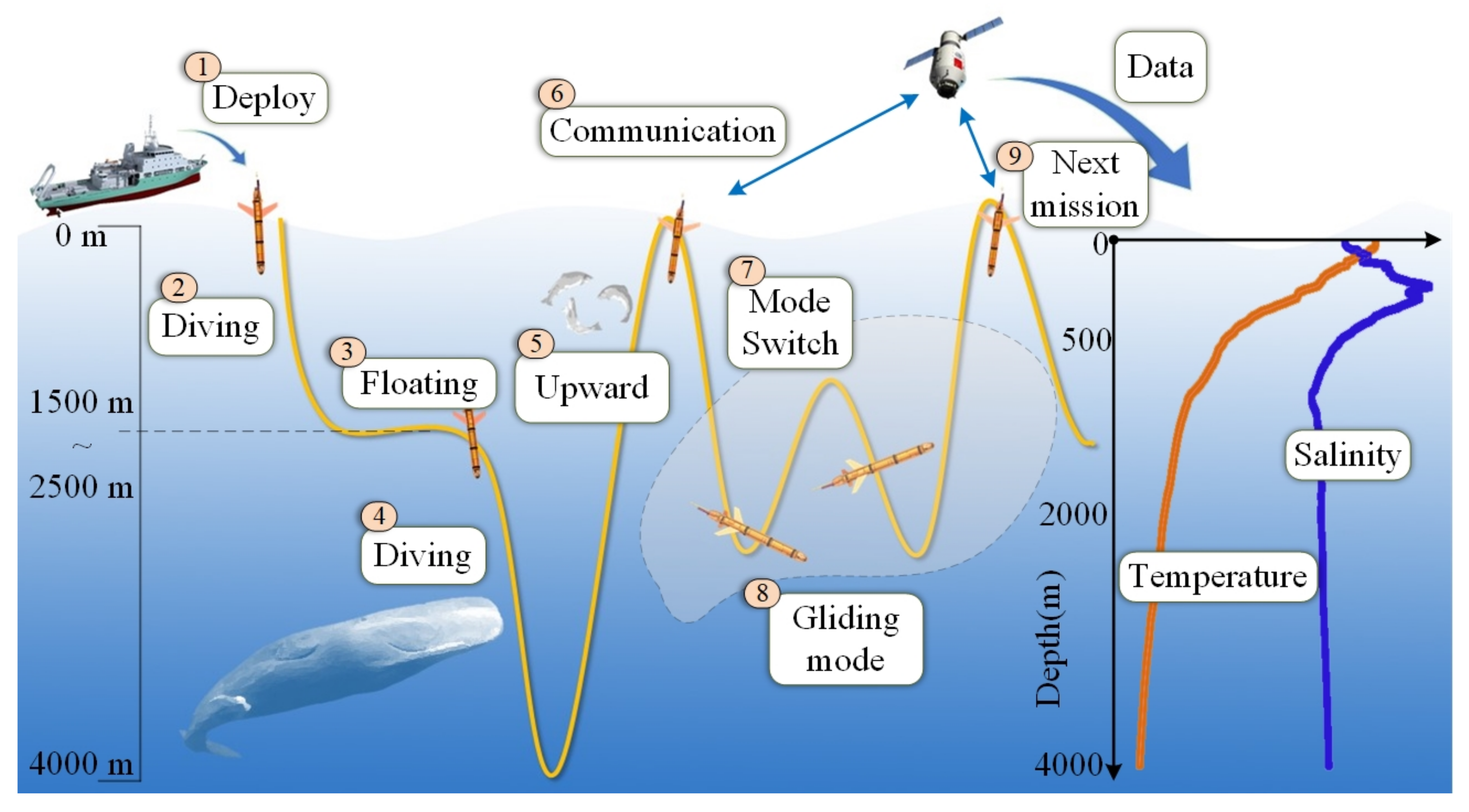
:1. Introduction
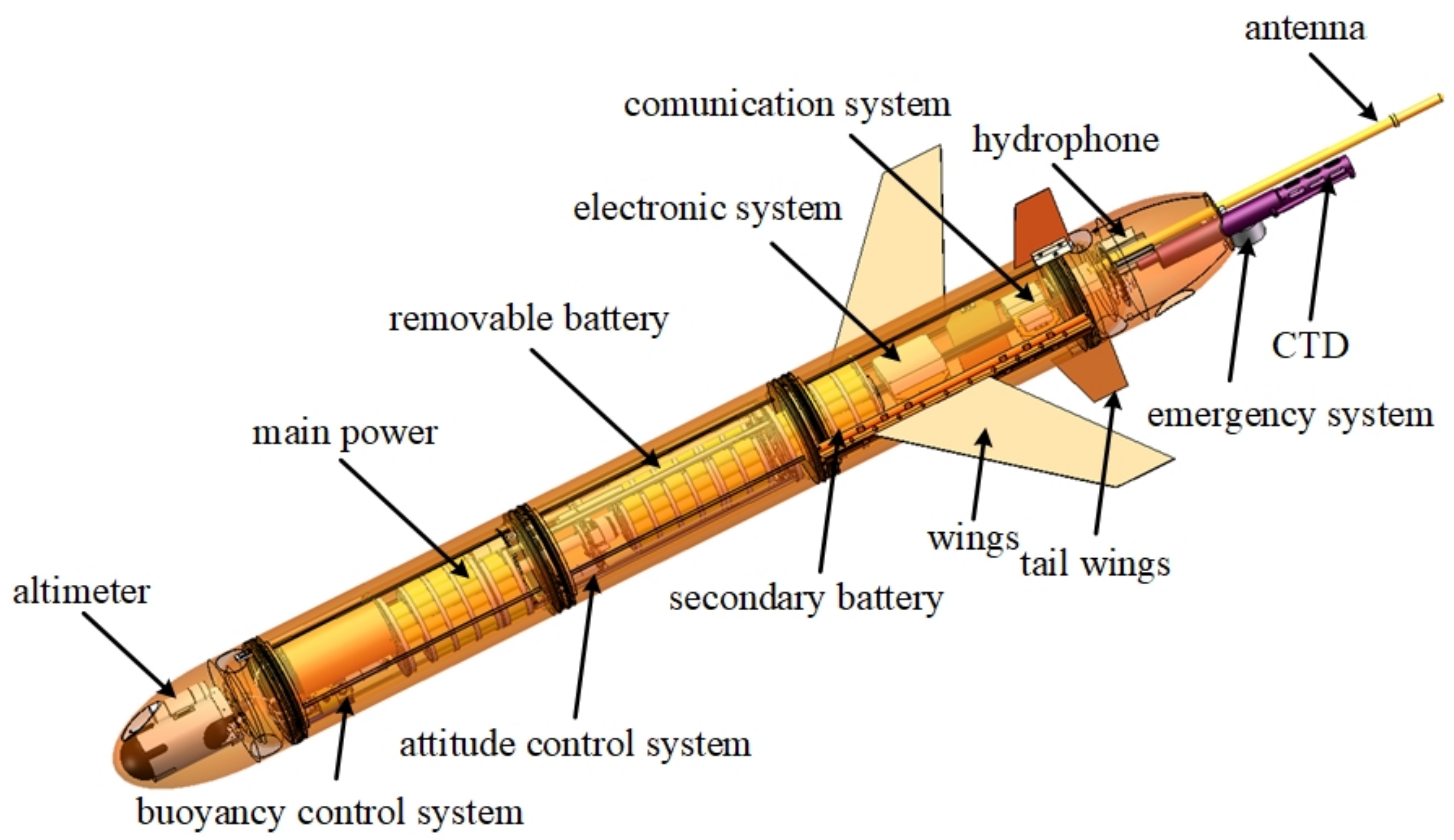
2. Dynamic Model for the Dual-Modal Underwater Vehicle
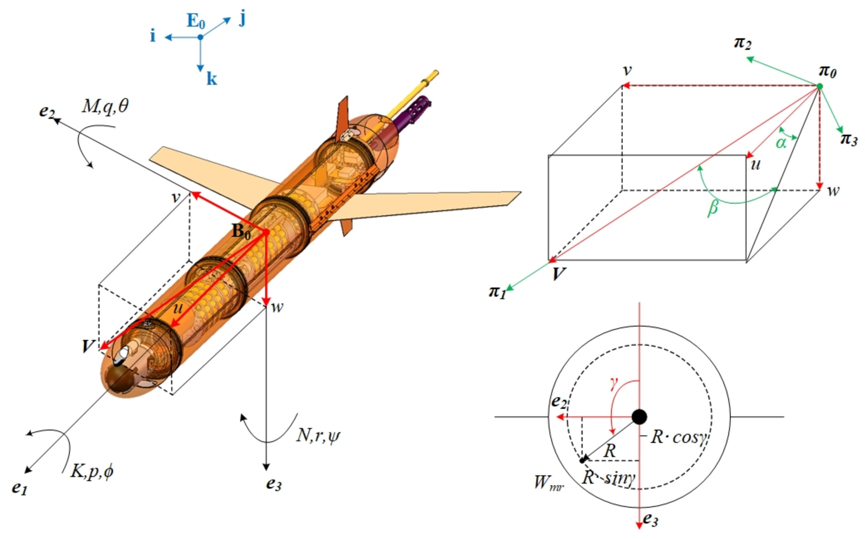
2.1. Coordinate Frames
- Rotate the body frame around the axis by , then the axis coincides with the axis;
- Rotate the frame around the axis by , then the axis coincides with the axis, and the axis coincides with the axis.
2.2. Model of Mechanics
2.3. Dynamic Model
2.4. Hydrodynamic Forces
3. Nonlinear MIMO Adaptive Backstepping Control
3.1. Assumptions
- The dynamic model of the vehicle was established in still water without disturbance caused by environment;
- The DUV had three planes of symmetry;
- The weak nonlinear terms and higher-order coupling terms in the dynamic model of DUV were neglected.
3.2. Controller Design
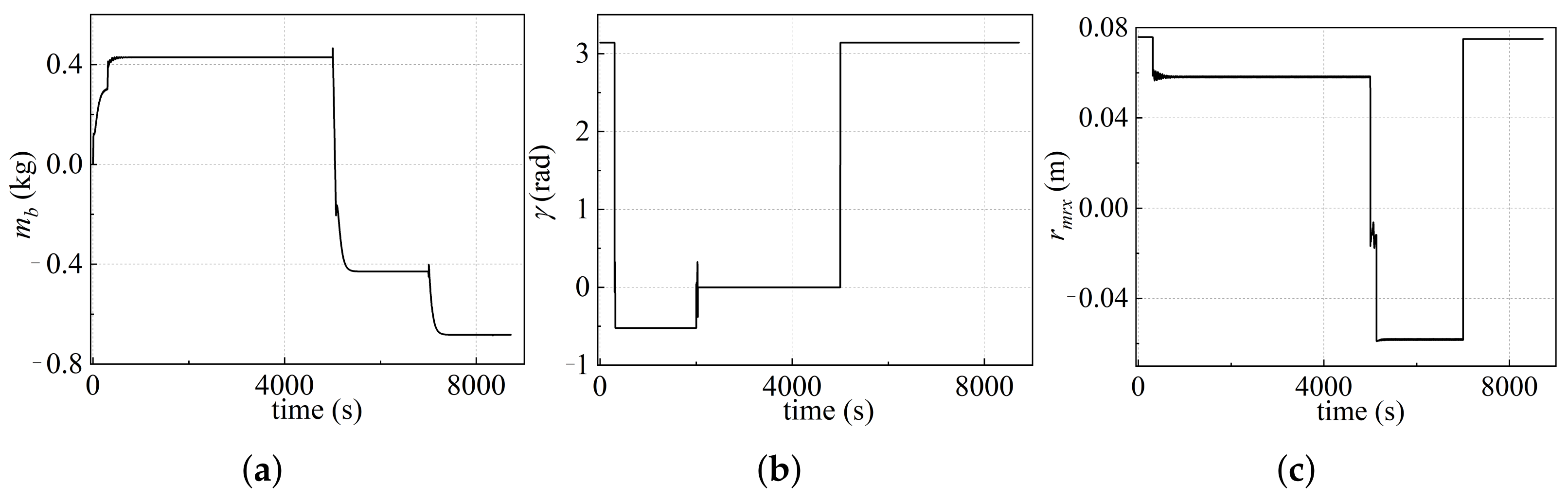
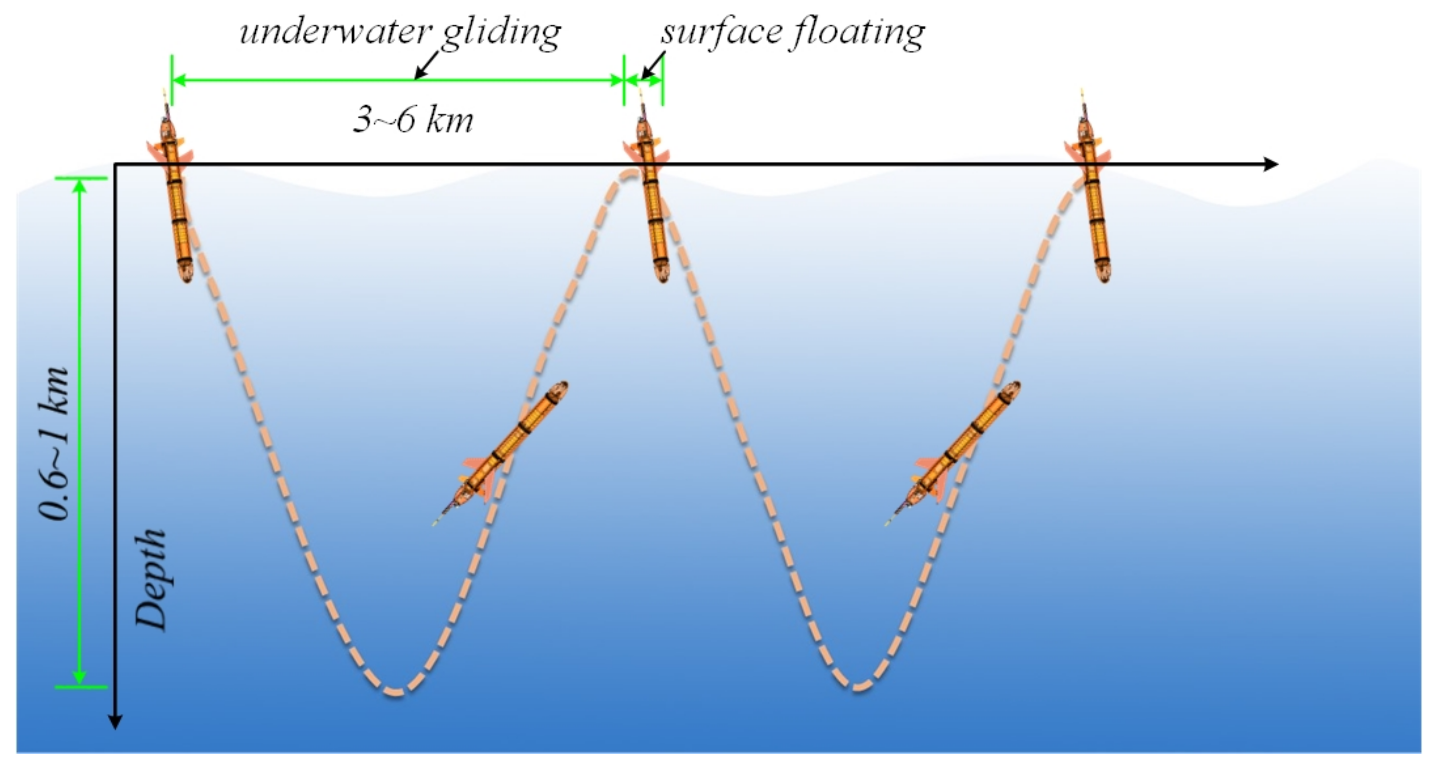
4. Characteristics and Analysis of Dual-Modal Motion
5. Sea Trials and Results
5.1. The Sea Test of the DUV in Single Mode
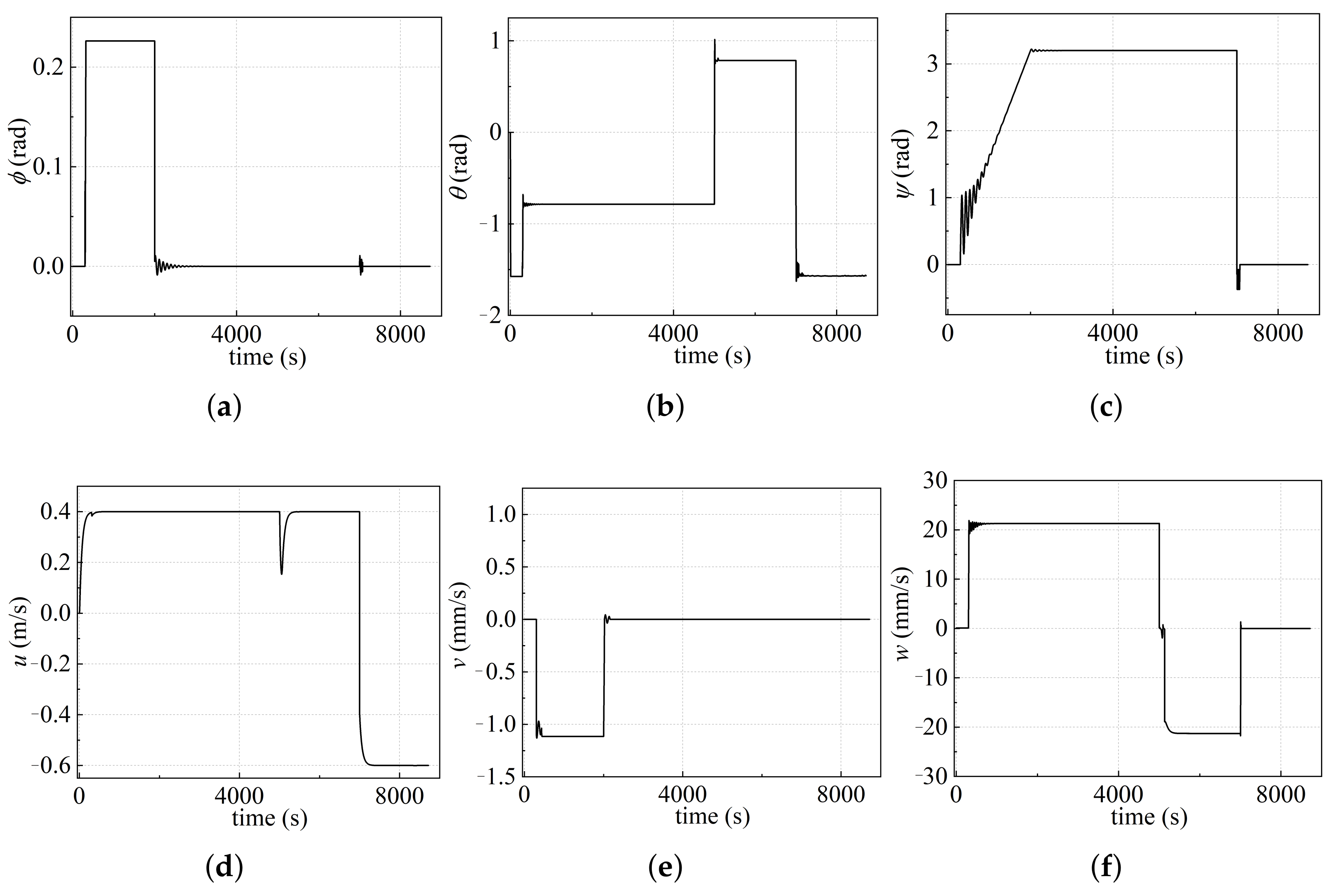
5.1.1. Course-Keeping Test of the DUV in Glider Mode
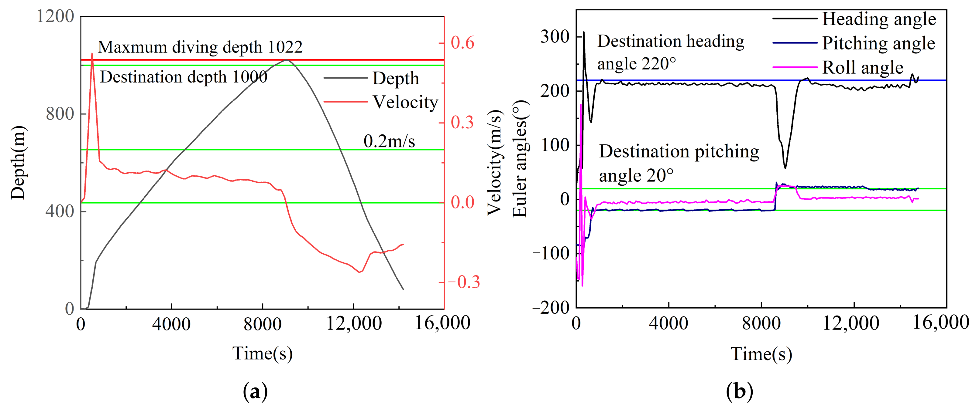
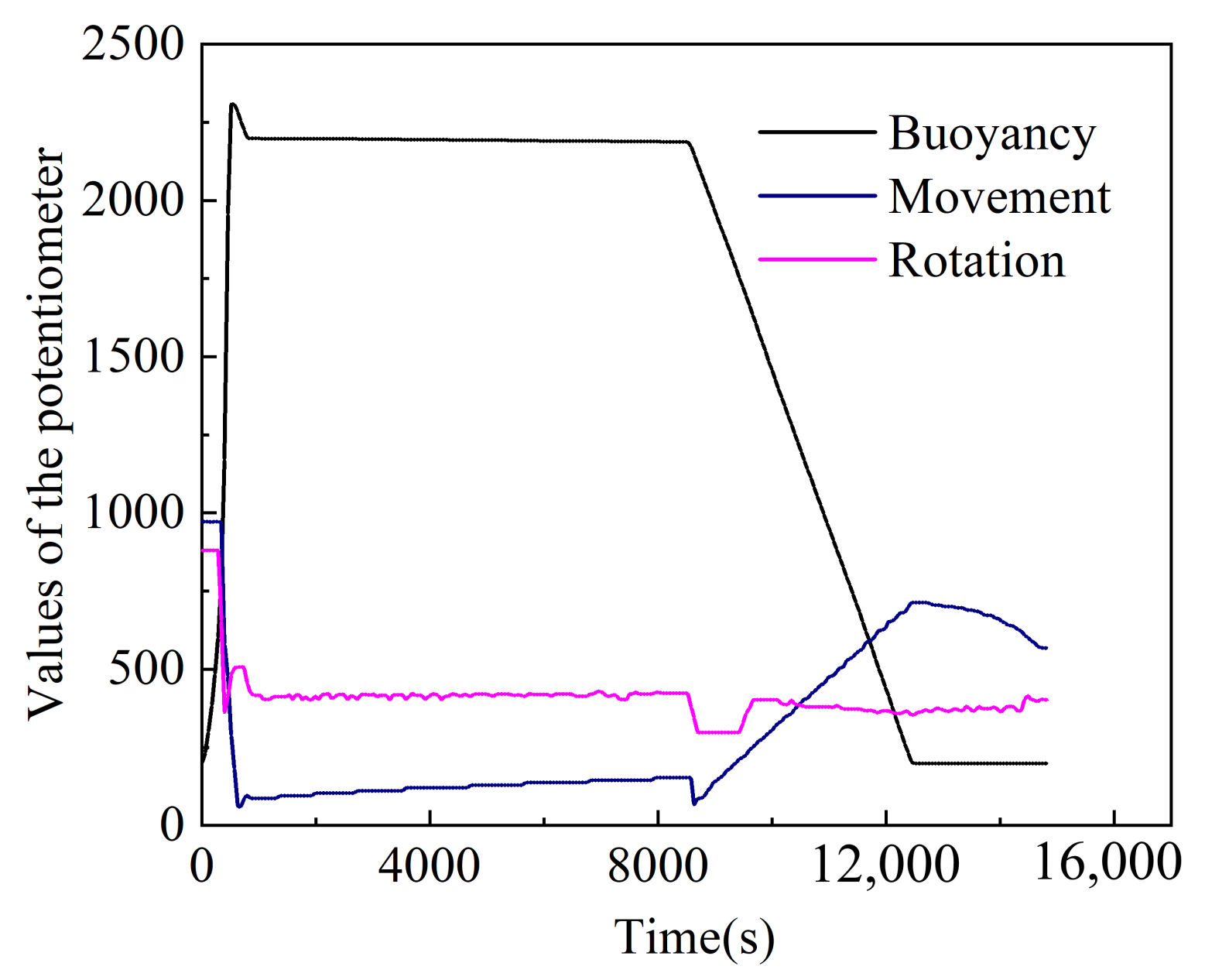
5.1.2. Diving Performance of the DUV in Argo Mode
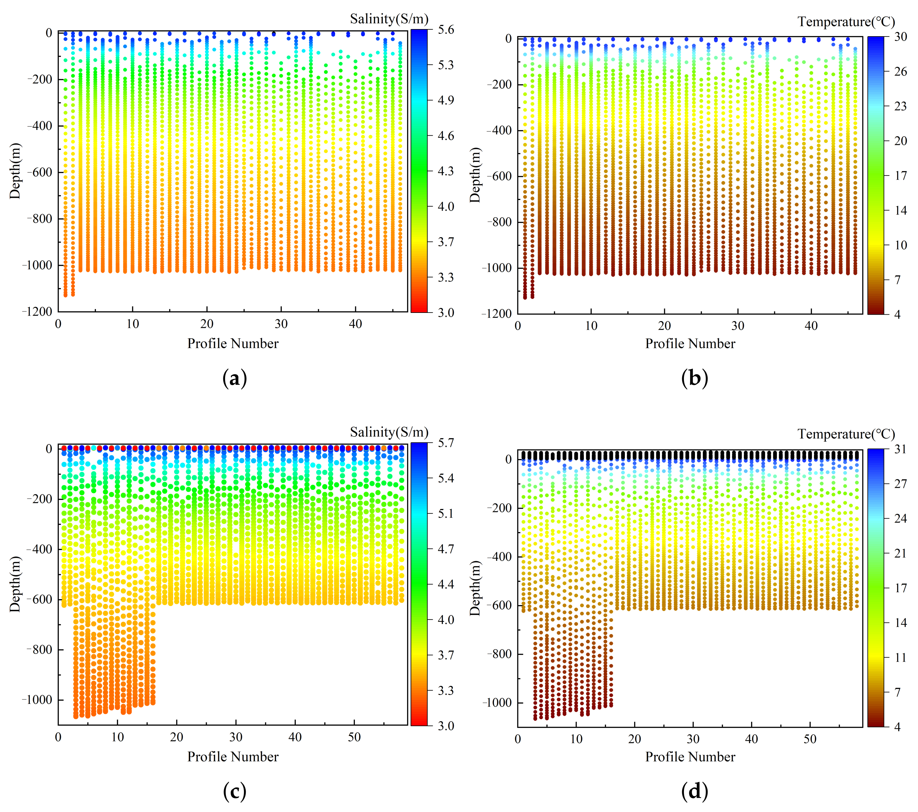
5.2. The Network Sea Test with Two DUVs
6. Conclusions and Discussion
Author Contributions
Funding
Institutional Review Board Statement
Informed Consent Statement
Data Availability Statement
Acknowledgments
Conflicts of Interest
Abbreviations
| DUV | Dual-modal underwater vehicle |
| AUV | Autonomous underwater vehicle |
| MIMO | Multi-input and multi-output |
| ABC | Adaptive backstepping contorl |
| HUG | Hybrid underwater vehicle |
| APDRC | Asia Pacific Data Research Center |
Appendix A

| Parameter | Value | Unit | Parameter | Value | Unit |
|---|---|---|---|---|---|
| 170.6 | kg | 20 | kg | ||
| [0.052,0,0.0057] | m | 3.25 | |||
| 103.45 | 104.06 | ||||
| 0.028 | m | mm | |||
| diag[2.12,15.4,1.85] | kg | ||||
| [0.015,0,00033] | m | m | 190.6 | kg | |
| 0.301 | m | 2.95 | m | ||
| 6.48 | kg | 95.58 | kg | ||
| 98.92 | kg | 3.55 | |||
| 44.88 | 40.18 | ||||
| 8.57 | 9.54 | ||||
| 18.6 | kg/m | 380.29 | kg/(m) | ||
| 0 | kg/m | 330.99 | kg/(m) | ||
| −160.65 | kg/(m) | −132.27 | kg/rad | ||
| −42.23 | 0 | kg/rad | |||
| −116.74 | kg/rad | −292.64 | |||
| 96.1 | kg/rad | −263.3 |
| Parameter | Explanation | Parameter | Explanation |
|---|---|---|---|
| the origin of inertial frame | the unit vectors of inertial frame | ||
| the origin of body frame | the unit vectors of body frame | ||
| the origin of flow velocity frame | the unit vectors of flow velocity frame | ||
| the position of vehicle in inertial frame | the components of | ||
| Euler angle in inertial frame | the components of | ||
| the velocity of vehicle in body frame | the components of | ||
| the velocity represented in body frame respected to current | the components of | ||
| the angular velocity in body frame | the components of | ||
| the attack angle | the drift angle | ||
| the rotation matrix from body frame to inertial frame | the rotation matrix from body frame to flow velocity frame | ||
| m | the total mass of DUV | the fixed mass, moving mass and variable mass of DUV | |
| the constant displacement mass of the DUV | the net mass of the vehicle | ||
| the positions of fixed mass, moving mass, and variable mass in inertial frame | the positions of fixed mass, moving mass, and variable mass in body frame | ||
| the matrix rotate around the axis | the component of the along the axis | ||
| the rotated angle of the movable mass | the eccentric distance of the moveable mass | ||
| the initial inertia matrix when | the rotational inertia matrix of fixed mass, moveable/rotateable mass and variable mass | ||
| the matrix of added mass, added inertial and coupled parameters | the velocity of the fixed mass, moving mass and variable mass in inertial frame | ||
| the angular velocity of the fixed mass, moving mass and variable mass in inertial frame | the third order identity matrix | ||
| the momentum and angular momentum in inertial frame | the momentum and angular momentum in body frame | ||
| the force and moment acting on the vehicle in inertial frame | the force and moment acting on the vehicle in body frame | ||
| D/X,/Y,L/Z | drag, drift force, vertical force | K/,M/,N/ | the moment components |
| ,, | the coefficients of vertical force, drift force and drag force | ,, | the coefficients of , , |
| g | acceleration of gravity | T | the total kinetic energy of the vehicle |
| , | the kinetic energy of fixed mass and moving mass | , | the kinetic energy of variable mass and added mass |
| the control input of system | the target control parameter of the system | ||
| the estimated value of | z | the difference between the state parameter value and estimated value |
References
- Li, D.H.; Wu, L.X.; Chen, Z.H. Strategic direction and construction path of transparent oceans. J. Shandong Univ. 2019, 2, 130–136. [Google Scholar]
- Liu, Z.H.; Wu, X.F.; Xu, J.P.; Li, H.; Lu, X.L. Fifteen years of ocean observations with China Argo. Adv. Earth Sci. 2016, 31, 1–16. [Google Scholar]
- Rudnick, D.L. Ocean Research Enabled by Underwater Gliders. Annu. Rev. Mar. Sci. 2016, 8, 519–541. [Google Scholar] [CrossRef] [PubMed]
- Cao, J.J.; Li, D.W.; Zeng, Z.; Yao, B.H.; Lian, L. Drifting and Gliding: Design of a multimodal Underwater Vehicle. In Proceedings of the IEEE OCEANS’2018 KOBE, Kobe, Japan, 28–31 May 2018. [Google Scholar]
- Zhao, W.T.; Yu, J.C.; Zhang, A.Q. The Cooperative Control Strategy for Underwater Gliders in Ocean Mesoscale Eddies Observation Task. Robot 2018, 40, 206–215. [Google Scholar]
- Xie, J.; Counillon, F.; Zhu, J.; Bertino, L. An eddy resolving tidal-driven model of the South China Sea assimilating along-track SLA data using the EnOI. Ocean Sci. 2011, 7, 609–627. [Google Scholar] [CrossRef] [Green Version]
- Li, Z.; Li, Y.P. Research on thermocline tracking based on dual autonomous underwater vehicles. Acm Int. Conf. Proc. Ser. 2018, 9, 122–127. [Google Scholar]
- Panda, P.J.; Mitra, A.; Warrior, H.V. A review on the hydrodynamic characteristics of autonomous underwater vehicles. J. Eng. Marit. Environ. 2021, 235, 15–29. [Google Scholar] [CrossRef]
- Hwang, J.; Bose, N.; Fan, S.S. AUV adaptive sampling methods: A review. Appl. Sci. 2019, 9, 3145. [Google Scholar] [CrossRef] [Green Version]
- Ullah, B.; Ovinis, M.; Baharom, M.B.; Javaid, M.Y.; Izhar, S.S. Underwater gliders control strategies: A review. In Proceedings of the 2015 10th Asian Control Conference (ASCC), Kota Kinabalu, Malaysia, 31 May–3 June 2015. [Google Scholar]
- Graver, J.G. Underwater Glider: Dynamics, Control and Design. Ph.D. Thesis, Princeton University, Princeton, NJ, USA, 2005. [Google Scholar]
- Wang, Y.H. Dynamical Behavior and Robust Control Strategies of the Underwater Gliders. Ph.D. Thesis, Tian Jin University, Tian Jin, China, 2007. [Google Scholar]
- Wang, S.X.; Liu, F.; Shao, S.; Wang, Y.H.; Niu, W.D.; Wu, Z.L. Dynamic modeling of hybrid underwater glider based on the theory of differential geometry and sea trails. J. Mech. Eng. 2014, 50, 19–27. [Google Scholar] [CrossRef]
- Yang, M.; Wang, Y.H.; Yang, S.Q.; Zhang, L.H.; Deng, J.J. Shape optimization of underwater glider based on approximate model technology. Appl. Ocean Res. 2021, 110, 102580. [Google Scholar] [CrossRef]
- Fan, S.S.; Woolsey, C.A. Dynamics of underwater gliders in currents. Ocean Eng. 2014, 84, 249–258. [Google Scholar] [CrossRef]
- Breivik, M.; Fossen, T.I. A unified control concept for autonomous underwater vehicles. In Proceedings of the American Control Conference, Minneapolis, MN, USA, 14–16 June 2006; pp. 4920–4926. [Google Scholar]
- Xiang, X.; Yu, C.; Zhang, Q.; Xu, G. Path-following control of an AUV: Fully actuated versus under-actuated configuration. Mar. Technol. Soc. J. 2016, 50, 34–47. [Google Scholar] [CrossRef]
- Niu, W.D. Stability Contorl and Path Planning for Hybrid-Driven Underwater Gliders. Ph.D. Thesis, Tian Jin University, Tian Jin, China, 2016. [Google Scholar]
- Noh, M.M.; Arshad, M.R.; Mokhtar, R.M. Depth and pitch control of USM underwater glider: Performance comparison PID vs. LQR. Indian J. Mar. Sci. 2011, 40, 200–206. [Google Scholar]
- Isa, K.; Rizal, A.M. Motion simulation for propeller-driven USM underwater glider with controllable wings and rudder. In Proceedings of the 2011 2nd International Conference on Instrumentation Control and Automation, ICA, Bandung, Indonesia, 15–17 November 2011; pp. 316–321. [Google Scholar]
- Wang, S.; Li, H.; Wang, Y.; Mokhtar, R.M. Dynamic modeling and motion analysis for a dual-buoyancy-driven full ocean depth glider. Ocean Eng. 2019, 187, 106163. [Google Scholar] [CrossRef]
- Yang, M.; Wang, Y.; Wang, S.; Mokhtar, R.M. Motion parameter optimization for gliding strategy analysis of underwater gliders. Ocean Eng. 2019, 191, 106502. [Google Scholar] [CrossRef]
- Yang, H.; Ma, J.; Mokhtar, R.M. Sliding mode tracking control of autonomous underwater glider. In Proceedings of the 2010 International Conference on Computer Application and System Modeling, Taiyuan, China, 22–24 October 2010; Volume 1, pp. 555–558. [Google Scholar]
- Liu, Y.; Ma, J.; Huang, Z. Numerical study on hydrodynamic behavior of an underwater glider. Ocean Eng. 2011, 6, 521–526. [Google Scholar]
- Cao, J.; Cao, J.; Zeng, Z. Nonlinear multiple-input-multiple-output adaptive backstepping control of underwater glider systems. Int. J. Adv. Robot. Syst. 2016, 13, 1–14. [Google Scholar] [CrossRef] [Green Version]
- Cao, J.J.; Lu, D.; Li, D.W.; Zeng, Z.; Yao, B.H.; Lian, L. Smartfloat: A Multimodal Underwater Vehicle Combining Float and Glider Capabilities. IEEE Access 2019, 7, 77825–77838. [Google Scholar] [CrossRef]
- Zhang, R.; Yang, S.; Wang, Y.; Yi, Y. Regional ocean current field construction based on an empirical bayesian kriging algorithm using dual underwater gliders. J. Coast. Res. 2020, 99, 41–47. [Google Scholar] [CrossRef]
- Xiao, H.; Zhang, Z.; Chen, L.; He, Q. An Improved Spatio-Temporal Kriging Interpolation Algorithm and Its Application in Slope. IEEE Access 2020, 8, 90718–90729. [Google Scholar] [CrossRef]


| Number | Deployment Time | Recovery Time | Average Depth | Profile Number |
|---|---|---|---|---|
| DUV1 | 24 April 2021 19:47:04 | 30 April 2021 12:30:44 | 1000 m | 23 |
| DUV2 | 25 April 2021 03:47:50 | 30 April 2021 11:32:30 | 600 m | 32 |
Publisher’s Note: MDPI stays neutral with regard to jurisdictional claims in published maps and institutional affiliations. |
© 2022 by the authors. Licensee MDPI, Basel, Switzerland. This article is an open access article distributed under the terms and conditions of the Creative Commons Attribution (CC BY) license (https://creativecommons.org/licenses/by/4.0/).
Share and Cite
Cao, J.; Lin, R.; Yao, B.; Liu, C.; Zhang, X.; Lian, L. Modeling, Control and Experiments of a Novel Underwater Vehicle with Dual Operating Modes for Oceanographic Observation. J. Mar. Sci. Eng. 2022, 10, 921. https://doi.org/10.3390/jmse10070921
Cao J, Lin R, Yao B, Liu C, Zhang X, Lian L. Modeling, Control and Experiments of a Novel Underwater Vehicle with Dual Operating Modes for Oceanographic Observation. Journal of Marine Science and Engineering. 2022; 10(7):921. https://doi.org/10.3390/jmse10070921
Chicago/Turabian StyleCao, Junjun, Rui Lin, Baoheng Yao, Chunhu Liu, Xiaochao Zhang, and Lian Lian. 2022. "Modeling, Control and Experiments of a Novel Underwater Vehicle with Dual Operating Modes for Oceanographic Observation" Journal of Marine Science and Engineering 10, no. 7: 921. https://doi.org/10.3390/jmse10070921
APA StyleCao, J., Lin, R., Yao, B., Liu, C., Zhang, X., & Lian, L. (2022). Modeling, Control and Experiments of a Novel Underwater Vehicle with Dual Operating Modes for Oceanographic Observation. Journal of Marine Science and Engineering, 10(7), 921. https://doi.org/10.3390/jmse10070921