Prediction of Cavitation Performance over the Pump-Jet Propulsor Using Computational Fluid Dynamics and Hybrid Deep Learning Method

Abstract

The cavitation performance of an oblique flow field is different from that under a pure axial flow field. This study analyzed the hydrodynamic performance, bearing force, and tip clearance flow field under different rotating speeds and different cavitation numbers in an oblique flow field. Furthermore, this study proposed a hybrid deep learning model CNN-Bi-LSTM to quickly and accurately predict the bearing force of a pump-jet propulsor (PJP), which will solve the problem of time-consuming calculation and consumption of considerable computing resources in traditional computational fluid dynamics. The Shear–Stress–Transport model and Reynolds-averaged Navier–Stokes equations were utilized to procure the training and testing datasets. The training and testing datasets were reasonably divided in the ratio of 7:3. The results show that the propulsion efficiency decreased more obviously under higher rotating speed conditions, with a maximum decrease of up to 13.59%. The small cavitation numbers 1.4721 and high oblique angle significantly impacted the efficiency reduction; the maximum efficiency loss exceeded 20%. Thus, a small cavitation number 1.4721 is extremely detrimental to the propulsion efficiency of the PJP due to the large cavitation area. Moreover, the intensity of the tip clearance vortex continuously increased with the rotating speed. The CNN-Bi-LSTM deep model successfully predicted the phase difference and trend change of the propulsor bearing force under different conditions. The prediction difference was large at the crest and trough of the bearing force, but it is within the acceptable error range.

1. Introduction

A pump-jet propulsor (PJP) differs from the traditional propeller. PJPs have been used in underwater autonomous vehicles (AUVs), and AUVs can sail in deep sea fields. Moreover, AUVs have high speed requirements. PJPs afford high propulsion efficiency and high speeds, which meets the needs of AUVs. However, the high speeds denote that PJPs are prone to cavitation in pure axial and oblique flows. PJPs are widely used in the military field, and consequently, little public literature exists on the hydrodynamic and cavitation performance of PJPs owing to their military purpose.

The numerical calculation of PJP is relatively easy to realize under the pure axial flow conditions, wherein the distribution of flow fields is uniform. Thus, most studies have analyzed the hydrodynamic and cavitation phenomenon of PJPs under pure axial flow. The author adopted experimental technology to study the hydrodynamic and cavitation properties at oblique flow angles (4.5°) [1,2]. They showed that the balance of the rotor and stator blades of PJP does not break under an oblique flow. The author used experimental technology to analyze the PJP hydrodynamic performance at different Reynolds number conditions [3]. The torque coefficient obtained using the mixed plane method well agreed with the experimental data. The author compared some differences in pressure fluctuations and tip clearance flow fields under different conditions using the computational fluid dynamics (CFD) and experimental methods [4,5]. For the numerical calculation method, studies have used numerical technology to study the hydrodynamic performance, which optimized the design scheme in the early PJP research [6,7,8,9]. With the development of computer technology, some researchers have employed the CFD method to analyze the hydrodynamic technology and cavitation properties of PJPs [10,11,12,13]. The author studied the hydrodynamic technology and tip clearance field performance of PJPs using the CFD method and Shear–Stress–Transport (SST) $k-\omega$ model, which also obtaining refined flow field results [14,15]. The author used the Reynolds-averaged Navier–Stokes (RANS) model to investigate the cavitation phenomenon and tip flow field performance of PJP [16], and they used the experimental method to verify the method feasibility. The author used the SST $k-\omega$ turbulence method and CFX simulation software to analyze the hydrodynamic performance, thrust coefficient, and torque coefficient of PJPs and verified the feasibility of the SST $k-\omega$ model in calculating the PJP flow field [17]. From the above literature, it can be seen that the k-omega SST model is a good choice for blading flow. The author used the panel method to establish a simulation model of the PJP steady-state flow field and proposed and verified a calculation model of the tip leakage vortex [18]. For the studies of oblique flow, they used the RANS method to analyze the velocity and pressure fields of PJPs under different oblique flow angles (0–20°) [19,20]. Their results showed that the oblique flow has a certain influence on the velocity field and torque of PJPs. The author used the detached-eddy-simulation (DES) turbulence method and the Z-G-B cavitation method to analyze the cavitation performance and hydrodynamic parameters of an unsteady flow field [21]. The author proposed a modified hybrid RAMS/LES model for unsteady calculations to determine the internal flow state of a PJP and the relation between the PJP and the external area [22]. The author investigated the influence of ducts and transition modeling for an unsteady flow field of a pre-swirl stator PJP [23]. They showed that the transition slightly changed the pressure fluctuation of the tip clearance region of rotor blades and duct trailing edge, which did not change the fluctuation frequencies.

The above literature on PJPs shows that the research on PJP has mainly focused on unsteady flow field performance at pure axial flow conditions using mainly adopted experimental methods and traditional numerical calculation methods. However, deep learning methods have been employed in fluid mechanics [24,25]. In the fluid prediction field, data-driven methods have been rapidly developed due to the generation of large amounts fluid data and the advancements in computer technology. In the early stage of research on flow field predictions, studies focused on predicting the airfoil and flow field around a cylinder and the application of different flow fields was studied later [26,27,28,29,30,31]. The author used a convolutional neural network (CNN) to predict the flow field around a cylinder and analyzed the difference between the CFD and predicted values from the vortex or velocity vector and vortex length perspectives [32]. To solve the problem of droplet drift caused by a single-rotor UAV flow field, the author used a generative adversarial network (GAN) to predict the UAV flow field and then used the flow field to analyze the relevant quantities [33]. Their deep learning model showed that the GAN model can utilize a previously generated flow field to generate a subsequent flow field. The author compared the predicted value of laminar diffusion flame and swirling stable flame with the real three-dimensional image using a deep learning method (CNN-LSTM), and their predictions well agreed with the three-dimensional image obtained by reconstructing the two-dimensional experimental image [34]. The author took advantage of data-driven method and combined the datasets obtained in a cavitation tunnel to predict the cavitation marine propeller generated noise spectra at the design-exploiting stage [35]. The author proposed a data-driven model to predict the velocity field of a scramjet isolator through the pressure field using a CNN and a super-resolution CNN [36]. The data-driven model successfully learned the relation between the velocity field and pressure on the scramjet isolator wall. In addition to the flow field prediction, the super-resolution reconstruction in flow fields [37,38,39,40] and fluid prediction methods considering physical information [41].

The above discussion shows that the current research on PJPs mainly focuses on the analysis of unsteady and cavitation flow fields under pure axial flow. Additionally, the research on the oblique flow angle is only limited to the unsteady flow field and exciting force. Furthermore, the influence of the cavitation flow field is very important under an oblique flow, and determining ways to quickly and accurately predict the time sequences flow field (such as excitation force) of PJPs is very important. This study is organized as follows. Section 1 presents the current research on PJPs and applications of deep learning in the fluid prediction aspect. Section 2 introduces CFD numerical methods and set-ups of PJP (such as geometric model, mesh, and boundary conditions). Section 3 introduces the design structures of the hybrid deep learning model and the generation method of the datasets. Section 4 shows the verification of the datasets’ accuracy and the verification CFD method. Section 5 analysis the hydrodynamic performance, bearing force, and tip clearance flow field under different rotating speeds and different cavitation numbers in oblique flow conditions. Moreover, the bearing force difference of the PJP between the predicted data and CFD method is studied. Finally, Section 6 presents the study conclusions.

2. CFD Numerical Technology and Set-Ups

2.1. Geometric Model of PJP

Figure 1 displays different geometric models of PJP. PJP can be classified into two different types depending on the stator: pre-swirl stator and pre-swirl rotor. Most previous studies have analyzed the pre-swirl-rotor-type PJP [11,14,15,19]. Herein, PJP is mainly applied in an AUV; thus, the pre-swirl-rotor-type PJP is considered herein. Tip clearance is located between the duct and rotor blades. Although the size of the tip clearance is very small, the flow field is very complicated, and it significantly impacts the flow field characteristics. The model parameters of PJP are shown in

Table 1. Model parameters of PJP.

Parameters	Values
Tip clearance size	$\delta$ = 0.5 mm
Rotor maximum diameter	$D_{\max }$ = 250 mm
Stator blade diameter	$D_s$ = 218 mm
Duct outlet diameter	$D_{d2}$ = 197 mm
Duct inlet diameter	$D_{d1}$ = 260 mm
Hub length	$L_h$ = 170 mm

.

2.2. Computational Domain and Mesh

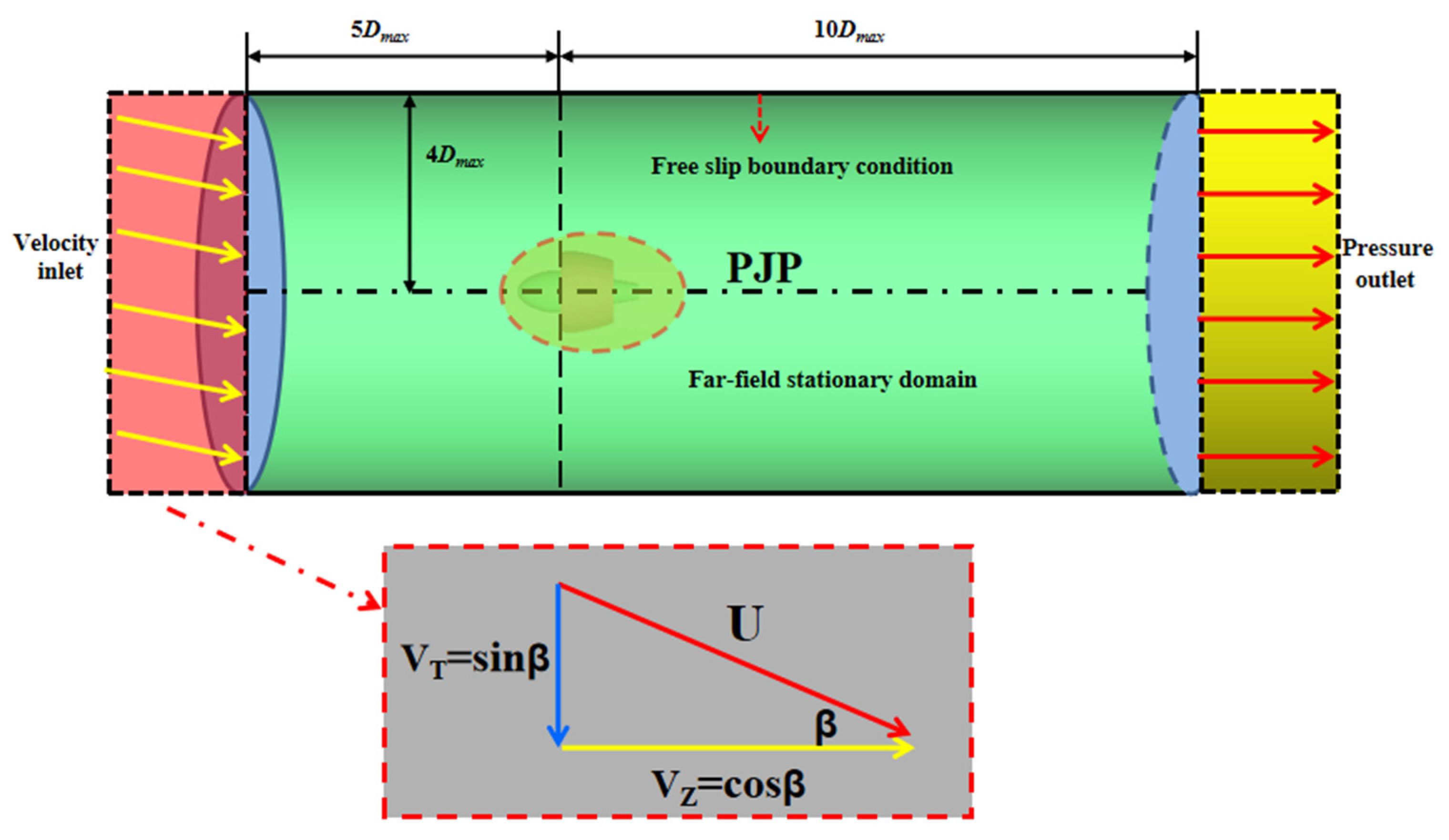
As shown in Figure 2, the cylinder computational domain with a radius of the 4 $D_{\max }$ was studied, extending from −5 $D_{\max }$ to 10 $D_{\max }$ in the streamwise direction, where $V_Z$ is the maximum diameter of the rotor blades (Table 1). The origin point of the coordinate is located at the entrance of the rotor blade. To simulate the PJP rotation, the entire cylinder computational domain is divided into three parts. The first part is rotation domain containing the rotor blades and rotor hub. The second is the stationary domain containing the stator blades, hubs, and duct. The third is the far-field domain that is set to the stationary domain. The interfaces are crucial for flow information exchange, and three pairs of interfaces are used herein. The bottom circle left side of the cylinder computational domain is set as the velocity inlet, and the distance from the origin point of the coordinates is 5 $D_{\max }$. The velocity is set to U = 15.72 m/s, and it is kept unchanged. The different advance ratios can be changed by varying the PJP rotating speed [14,19]. For pure axial flow conditions ($\beta =0^{\circ }$), the distribution of profile and turbulent kinetic energy TKE is uniform. The velocity value in the far-field region is relatively small, and the value in the near-field region is relatively large. For oblique flow ($\beta ={10}^{\circ },{20}^{\circ }$), the distribution of profile and turbulent kinetic energy TKE is not uniform. The larger the oblique flow angle, the distribution of in-homogeneity is larger. The bottom circle right side is set to the pressure outlet, where the distance is 10 $D_{\max }$. Additionally, the pressure outlet with an operating pressure of 0 Pa is set as the boundary conditions. The sides of the cylinder computational domain are set as the free slip wall boundary conditions. The no-slip wall boundary conditions include the rotor blades, stator blades, ducts, and hubs. According to Lu et al. (2020), the time step is 5.208 × 10⁻⁵ when the rotating speed R = 3200 rpm. Other time steps are 8.33 × 10⁻⁵, 6.41 × 10⁻⁵, 4.63 × 10⁻⁵, and 4.17 × 10⁻⁵ when the speeds are 2000, 2600, 3600, and 4000 rpm, respectively.

Compared to the study of the pure axial flow of the PJP, two methods can be used to numerically calculate the PJP under oblique flow conditions. In the first method, the position of the rotating domain is adjusted to adapt to the different oblique flow angles of the PJP [20]. In the second method, the velocity component of the coming flow is adjusted [19,42]. The two methods afford good calculation results, as shown in previous studies. However, the first method is tedious, and in it, each oblique flow angle condition needs to be adjusted in the PJP simulation model. To save the workload, the second method is adopted herein. The author compared the effects of these two boundary conditions, thus comparing the bearing force under the condition of oblique flow. It also can be seen from Figure 3 that the difference of vertical force under the two boundary conditions is relatively small [19]. Different oblique flow angles can be realized by changing the angle of attack of the incident flow of the horizontal plane x–z. Here, U denotes the inflow velocity, β denotes the oblique flow angle, $V_Z$ denotes the axial velocity component, and $V_T$ denotes the tangential velocity component. The density of water is $1\times {10}^3\mathrm{kg}/{\mathrm{m}}^3$, the temperature of the water is set to 25 °C.

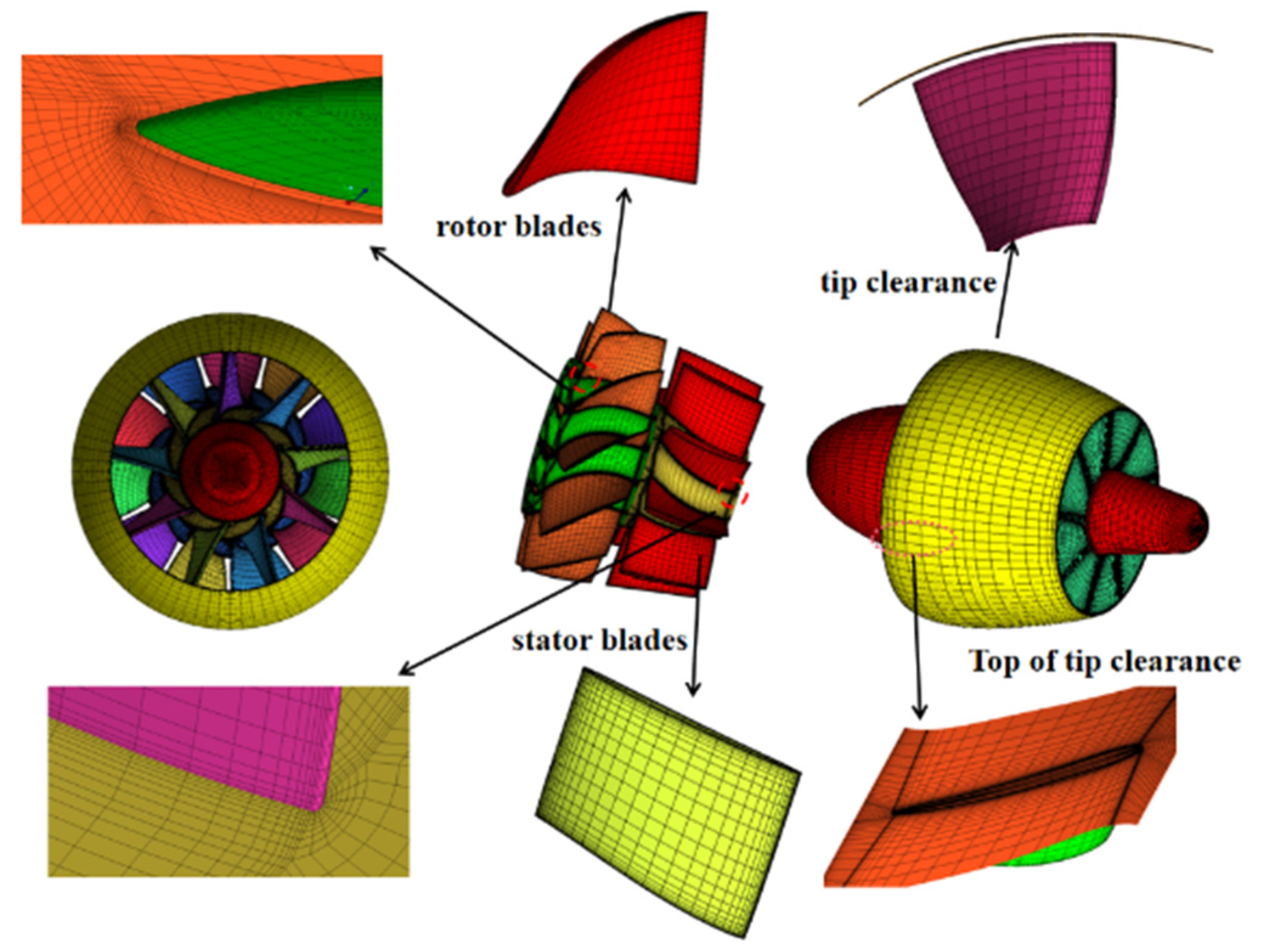
Figure 4 displays the detailed tip clearance grid and the detailed grid of the PJP. The duct wall can surround the axial HC-Block type grid and circumferential O-Block meshes. The O-Block meshes are used on the surface of the rotor and stator blades. The flow field between the tip clearance is more complicated compared to that in the other areas. Figure 4 shows that the grid of the tip clearance area is very dense, and thus, the double layers “O” topological mesh is adopted in this area to encrypt the grid. The height of the first grid is 4.1 × 10⁻⁵ m, which satisfied the y⁺ value (30–100) required by the turbulence model SST $k-\omega$ (Section 2.3) under the high Reynolds number condition. The total number of grids is 1.662 × 10⁷. In this study, Fluent in CFD software was used to calculate the cavitation flow field of PJP.

2.3. The Basic Equation

The RANS equations are adopted herein. Moreover, the SST $k-\omega$ turbulence model is used in the study of traditional propellers [43,44] and the research of PJP [5,12,14,15,16,19,45,46]. The previous studies have shown that the SST $k-\omega$ turbulence model has good applicability in the numerical simulation of the PJP. Furthermore, the SST $k-\omega$ turbulence model is a hybrid model; it combines the advantages of the $k-\epsilon$ model and the $k-\omega$ turbulence model [47]. The advantage of the $k-\omega$ turbulence model is the calculation accuracy of the near wall region, and the advantage of the $k-\epsilon$ model is the calculation accuracy of the far flow field. The SST $k-\omega$ turbulence model has a strong applicability as the turbulent shear stress evacuation process is also considered in the definition of the turbulent viscosity process. The author compared the hydrodynamic performance differences of the PJP among the three turbulence models: SST $k-\omega$, standard $k-\epsilon$, and Realizable $k-\epsilon$ turbulence model [45]. They showed that that the SST $k-\omega$ turbulence model afforded the smallest hydrodynamic performance errors. Equations (1) and (2) present its closed equations. Where, the asterisks represent specific parameters.

$$\frac{\partial k}{\partial t}+\nabla •(Uk)=\tilde{G}-{\beta }^{\ast }k\omega +\nabla •\left[(\nu +{\alpha }_k{\nu }_t)\nabla k\right],$$

(1)

$$\frac{\partial \omega }{\partial t}+\nabla •(U\omega )=\gamma S^2-\beta {\omega }^2+\nabla •\left[(\nu +{\alpha }_{\omega }{\nu }_t)\nabla \omega \right]+(1-F_t)C{D}_{k\omega }$$

(2)

The definition of F₁ is as follows:

$$F_t=\tanh \left\{{\left[\min (\max (\frac{\sqrt{k}}{{\beta }^{\ast }\omega y},\frac{500\nu }{y^2\omega }),\frac{4{\alpha }_{\omega 2}k}{C{D}_{kw}^{\ast }{y}^2}\right]}^4\right\},$$

(3)

$$C{D}_{\mathrm{kw}}^{\ast }=\max (2{\sigma }_{\omega 2}\nabla k•\frac{\nabla \omega }{\omega },{10}^{-10}),$$

(4)

$$\tilde{G}=\min \left\{{\nu }_t{S}^2,c_1{\beta }^{\ast }k\omega \right\},$$

(5)

where ${\nu }_t{S}^2$ is a generated term; $S=\sqrt{2S_{ij}{S}_{ij}}$ is the invariant measure of the stain rate, and $S_{ij}$ is the strain rate tensor. An asterisk represents an item with a specific parameter. The turbulent viscosity ${\nu }_t$ is shown in Equation (6):

$${\nu }_t=\frac{{\alpha }_{1}k}{\max ({\alpha }_1\omega ,S{F}_2)},$$

(6)

where $F_2=\tan \left\{{\left[\max (\frac{2\sqrt{k}}{{\beta }^{\ast }\omega y},\frac{500\nu }{y^2\omega })\right]}^2\right\}$ is the second mixture equation.

Additionally, $\phi ={\phi }_1{F}_1+{\phi }_2\left(1-F\right)$ is the other coefficient, where $\phi$ is the mixing coefficient; ${\phi }_1$ and ${\phi }_2$ represent the coefficients in the $k-\omega$ model and $k-\epsilon$ equations.

Table 2. Coefficients for turbulence model.

αk1	αω1	αω2	${\mathit{c}}_1$	β2	γ1	γ2
0.85034	0.5	0.85616	0.075	0.0828	0.5532	0.4403

illustrates the coefficients of the model.

They used the Z-G-B (Zwart-Gerber-Belamri) cavitation model to study PJP [16,21]. The Z-G-B model equations are as follows:

$$m^{+}=F_e\frac{3r_{muc}(1-{\alpha }_v)P_v}{R_B}\sqrt{\frac{2}{3}\frac{P_v-P}{P_l}},$$

(7)

$$m^{-}=F_c\frac{3{\alpha }_v{\rho }_v}{R_B}\sqrt{\frac{2}{3}\frac{P_v-P}{P_l}},$$

(8)

where $m^{+}$ and $m^{-}$ are the vaporization and condensation coefficients, respectively. $F_e$ and $F_c$ denote the vaporization and condensation indices, respectively: $F_e$ = 50 and $F_c=50$. $R_B$ denotes the radius of a vapor bubble: $R_B$ = 10⁻⁶. $r_{nuc}$ is the vapor volume fraction: $r_{nuc}=5\times {10}^{-4}$; ${\alpha }_v$ denotes the vapor phase.

$$p_v=p_{sat}+\frac{p_{turb}}{2},$$

(9)

$$p_{turb}=0.39{\rho }_{m}k.$$

(10)

Here, $p_{sat}$ represents the vapor pressure and $k$ is the turbulent energy.

3. Deep Learning Methods and Set-Ups

3.1. Hybrid Deep Learning Model CNN-Bi-LSTM

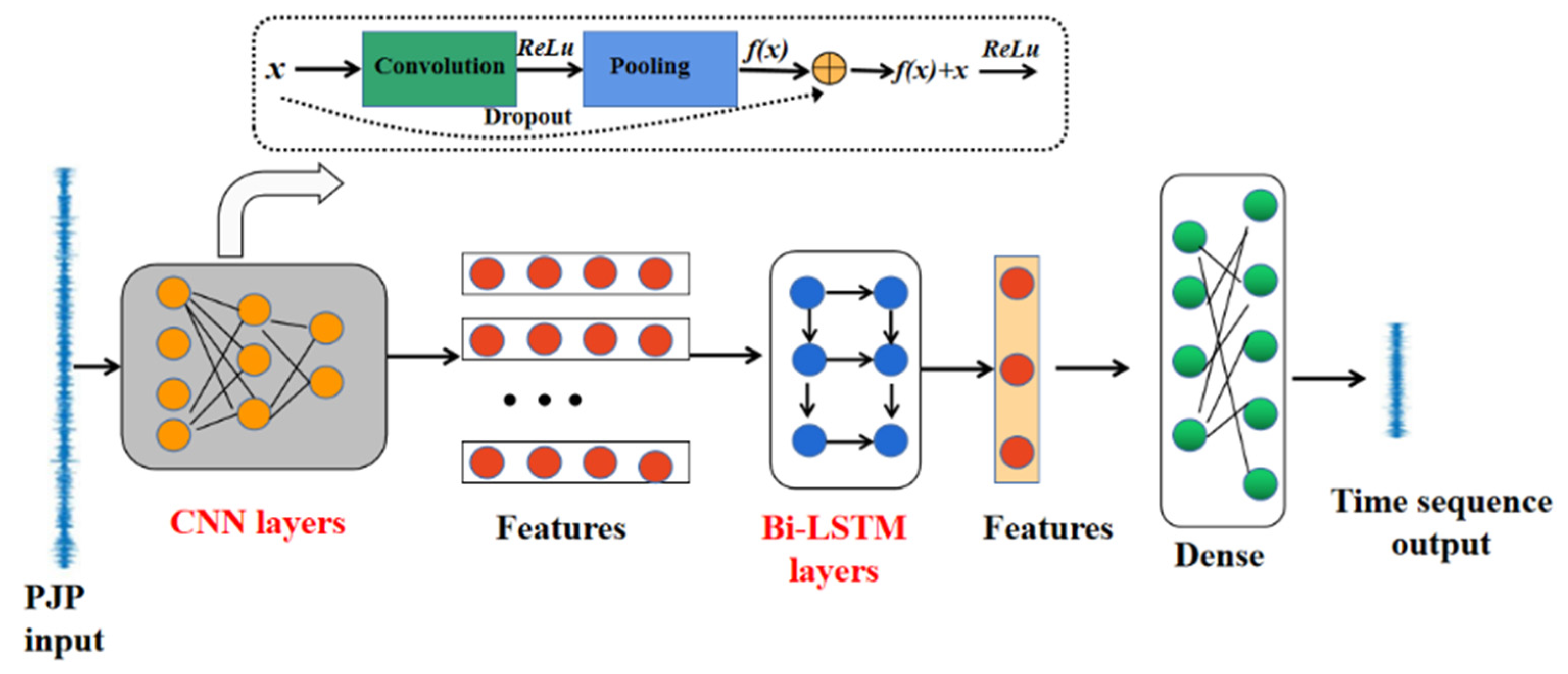
Deep learning methods have been employed in rotating machinery [35,48,49]. Most of them use a single neural network, such as CNN and long and short-term memory network (LSTM). CNN can well extract local features in time or space, but it lacks the ability to learn the correlation of the time sequence, and thus, it cannot solve the problem of long-term dependence based on the considerable information. Although LSTM can solve the problem of long-term dependence, it does not fully consider the impact of future characteristic information as LSTM only reads the sequence data in one direction. Herein, a CNN-Bi-LSTM hybrid model is proposed that combines CNN and bidirectional LSTM (Bi-LSTM), fully utilizing both their respective advantages. Figure 5 displays the process of the CNN-Bi-LSTM hybrid model. The hyperparameter combination was obtained through various attempts, yielding high accuracy and generalization ability.

Table 3. Parameters of the different layers of the CNN-Bi-LSTM model.

Name of Layer	Filters
Conv1	64 × 1
Dropout	0.05
Pooling layer 1	16 × 1
Conv2	32 × 1
Pooling layer 2	8 × 1
Conv3	16 × 1
Pooling layer 3	8 × 1
Flatten	/
Bi-LSTM 1	300
Bi-LSTM 2	200
Bi-LSTM 3	150
Dense	100
Dense	1

displays the parameters of the different layers.

3.2. 1D-CNN Structure and Bi-LSTM Structure

A fully connected neural network (FCN) can require considerable training time due to the large number of nodes and bias vectors, and CNN well solves this problem. The author proposed the first successful deep network. Herein, 1D-CNN is used as the training and testing datasets are time series features for PJP [50]. The 1D-CNN mainly comprises input layer, convolutional layer (Conv), pooling layer, fully connected layers, and output layer.

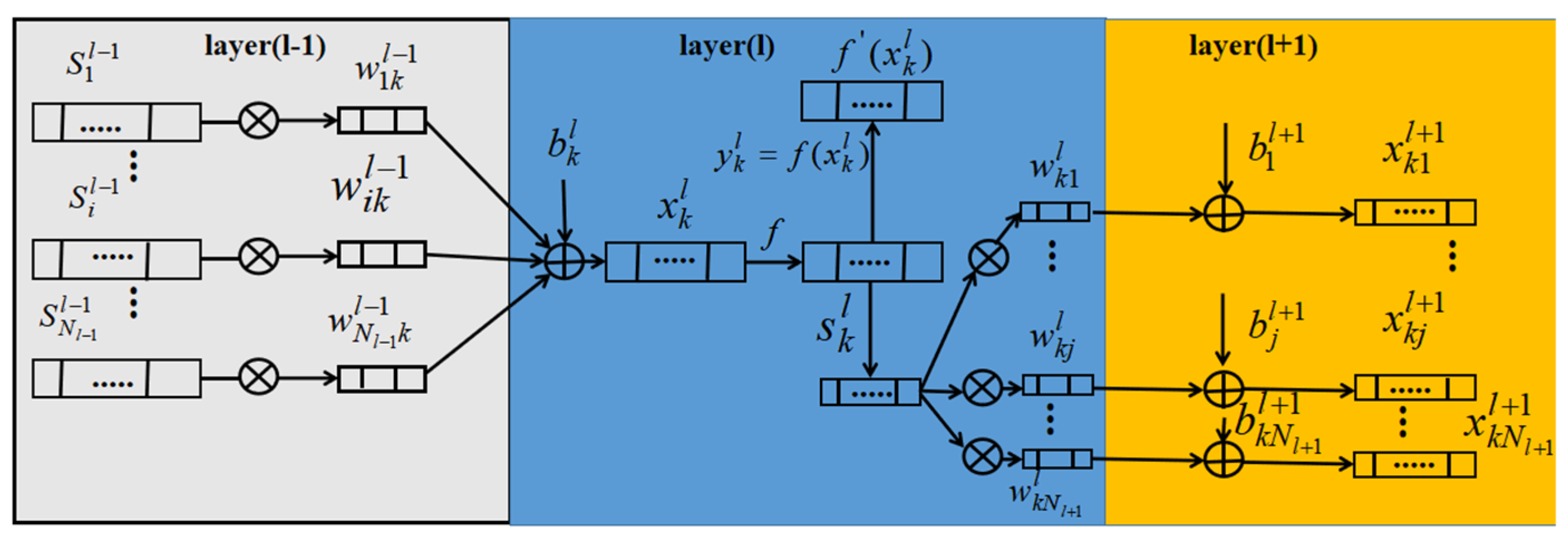
The convolutional and pooling layers are used to extract data features. Deeper features of the time sequences will be extracted when the number of layers is increased, but the convergence time will be prolonged. However, the accuracy of the neural network will reduce if the number of layers is reduced. Three convolution and pooling layers have been adopted herein. Figure 6 exhibits the operation process of the 1D-CNN. The operating formula of the 1D-CNN convolution is shown in Equations (11) and (12).

$$x_k^l={\displaystyle \sum _{i=1}^{N_{l-1}}Conv1D({\omega }_{ik}^{l-1},s_i^{l-1})+}{b}_k^l,$$

(11)

$$y_k^l=f(x_k^l)=\max (0,x_k^l).$$

(12)

Here, $f()$ is the activation function, and $y_k^l$ is the output of $x_k^l$. Conv1D represents the convolution operation.

After the convolution operation, the number of feature sequences can be increased, which will increase the data dimension. Additionally, it will increase the calculation complexity. Thus, the dimension needs to be reduced using the maximum pooling layer, as shown in Equation (13). The cross-entropy loss function is shown in Equation (14).

$$s_k^l=\max (y_k^l(2n-1),(y_k^l(2n)),n=1,2,3,\text{.......},m/2$$

(13)

$$E(j)=-{\displaystyle \sum _{i=1}^q{y}_i^{(j)}}\log {\hat{y}}^{(j)}$$

(14)

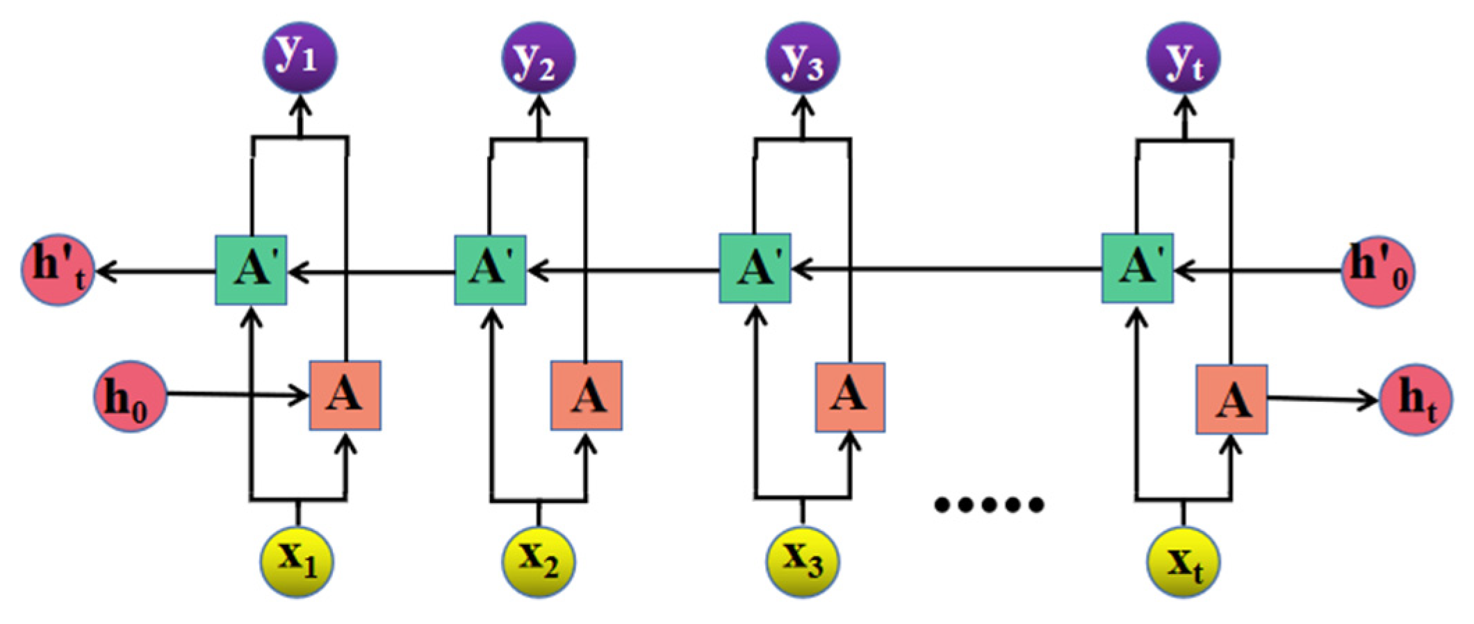
Bi-LSTM is a combination of forward and backward LSTM, as shown in Figure 7. Single-LSTM has been well explained in other studies, and it will not be elaborated on herein. The forward and reverse LSTM hidden layers are responsible for the forward and reverse feature extractions, respectively. The Bi-LSTM model can better consider the influence of before and after attributes of each attribute point in the sequence data than the single-LSTM model. The forward process of the Bi-LSTM model is denoted by Equations (15)–(20), and the backward process is the same as the forward process.

$$i_t=\sigma ({\omega }_i•[h_{i-1},P_t]+b_i)$$

(15)

$$f_t=\sigma (w_f•[h_{t-1},P_t]+b_f)$$

(16)

$${\tilde{C}}_t=\tanh (w_c•[h_{t-1},P_t]+b_c)$$

(17)

$${\overrightarrow{C}}_t=f_t\times {\overrightarrow{C}}_{t-1}+i_t\times {\overrightarrow{C}}_t$$

(18)

$$O_t=\sigma (w_o•[{\overrightarrow{h}}_{t-1},P_t]+b_o)$$

(19)

$${\overrightarrow{h}}_t=O_t\times \tanh ({\overrightarrow{C}}_t)$$

(20)

3.3. Division of the Time Sequence Datasets

Both the training and testing datasets are derived from the numerical simulation data of the PJP. The training and testing datasets were divided in the ratio of 7:3. The datasets comprise 15,380 time-step flow field data of the PJP, with 11,060 and 4740 time-steps for the training and testing datasets. The datasets are mainly derived from the time series of the PJP bearing force.

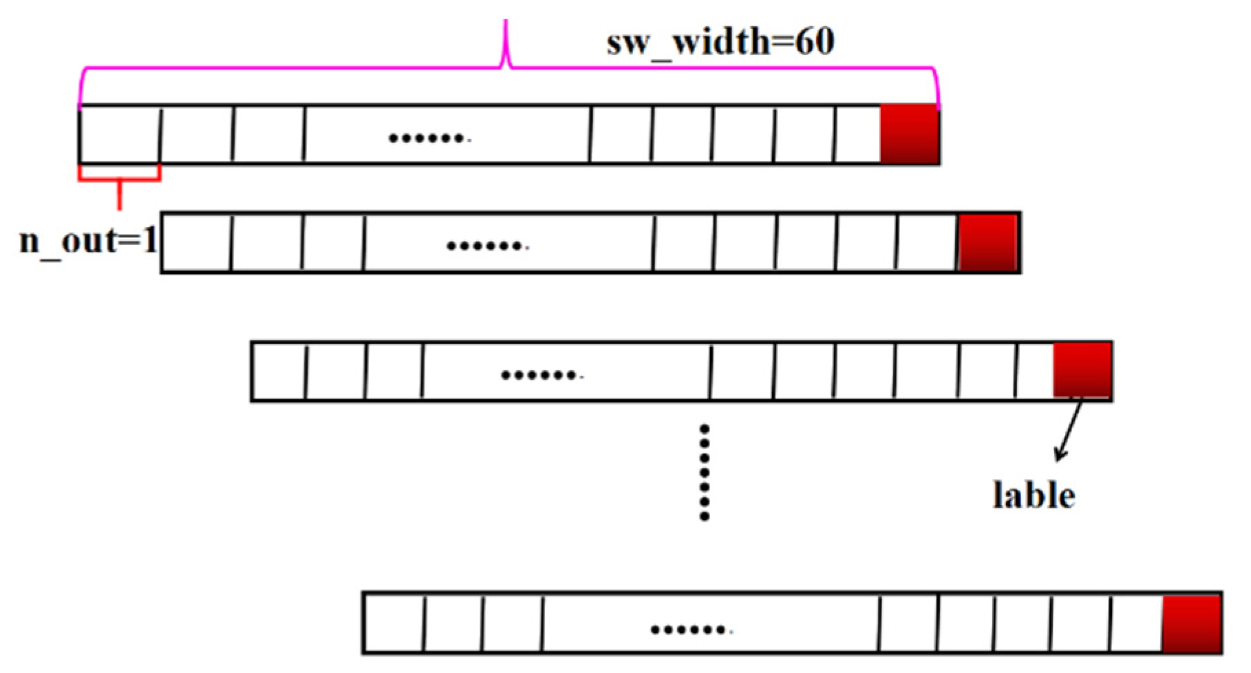
After various training and trials, a learning rate of 0.001 and the Adam optimization algorithm are adopted. The mean square error function is employed to evaluate the CNN-Bi-LSTM model performance. The TensorFlow platform is used for training and testing the deep model. The datasets are a time sequence without labels. The CNN-Bi-LSTM deep model is a supervised learning model, which requires a sliding window to obtain the time series features with labels. As shown in Figure 8, the sliding window width (sw_width) is set as 60 and the sliding step (n_out) is set as 1 to form a new time-variable sequence with labels.

4. Model Verification

4.1. Vertification of the Accuracy of the Datasets

For a more convenient comparison of the numerical calculation and experimental results, some non-dimensional physical quantities are employed (

Table 4. Non-dimensional quantities of PJP.

Physical Quantities	Definition
Thrust coefficient	$K_T=\frac{T}{\rho n^2{D}^4}$
Torque coefficient	$K_Q=\frac{Q}{\rho n^2{D}^5}$
Open water efficiency	$\eta =\frac{J}{2\pi }\frac{K_T}{K_Q}$
Advance ratio	$J=\frac{V}{nD}$

).

The accuracy of the datasets is extremely important for PJP prediction performance. A relatively large prediction error of the datasets will cause the pollution of the training datasets, which will reduce the generalization ability. The applicability of the SST $k-\omega$ and Z-G-B models will affect the accuracy of the datasets; thus, CFD is adopted here. They used the Ka4-70 ducted propeller to verify the method [19,23,46]. Furthermore, the author compared the numerical approach results of the SST $k-\omega$ turbulence model and the sliding mesh technique with the PJP experiment results [4], and the results showed good agreement. The above example demonstrates a good applicability of the numerical method in PJP. Herein, the PJP geometric model of [23] is selected to verify the numerical simulation method. The numerical simulation and experimental data [23] are shown in

Table 5. Error between the CFD and experimental (Exp) results.

Advance Ratio J	η (CFD)	η (Exp)	Δη (%)
1.58	0.5582	0.5379	3.64
1.76	0.591	0.579	2.03
1.92	0.6122	0.6044	1.27
2.11	0.6275	0.6125	2.39
2.26	0.6294	0.6199	1.51
2.43	0.6216	0.6154	0.99
2.64	0.5992	0.5892	1.67
2.75	0.5774	0.5635	2.41
2.87	0.5421	0.5408	0.24
3.16	0.4281	0.4153	2.99
3.33	0.3206	0.3058	4.83
3.51	0.1773	0.1769	0.23

. In Table 5, the error $\Delta \eta$ between all the experimental and CFD results are within the 5% range. The above comparison verifies that the numerical method of this study has good applicability for PJP prediction.

The

Table 6. The error of $K_{Ts}$ and $K_{Qs}$.

Advance Ratio J	(CFD)	(Exp)	Error (%)
1.4 ($K_{Ts}$)	0.6621	0.6546	1.15
1.4 ($K_{Qs}$)	0.2743	0.2713	1.11
1.5 ($K_{Ts}$)	0.6723	0.6812	1.31
1.5 ($K_{Qs}$)	0.2733	0.2687	1.71
1.6 ($K_{Ts}$)	0.6792	0.6703	1.33
1.6 ($K_{Qs}$)	0.2698	0.2655	1.97

shows the error $K_{Ts}$ and $K_{Qs}$ between CFD values and experimental values at different advance ratio J. The error $K_{Ts}$ and $K_{Qs}$ are all within 2%. From the point of view of thrust coefficient $K_{Ts}$ and torque coefficient $K_{Qs}$ of PJP, which proves that this method is also suitable for numerical simulation of PJP.

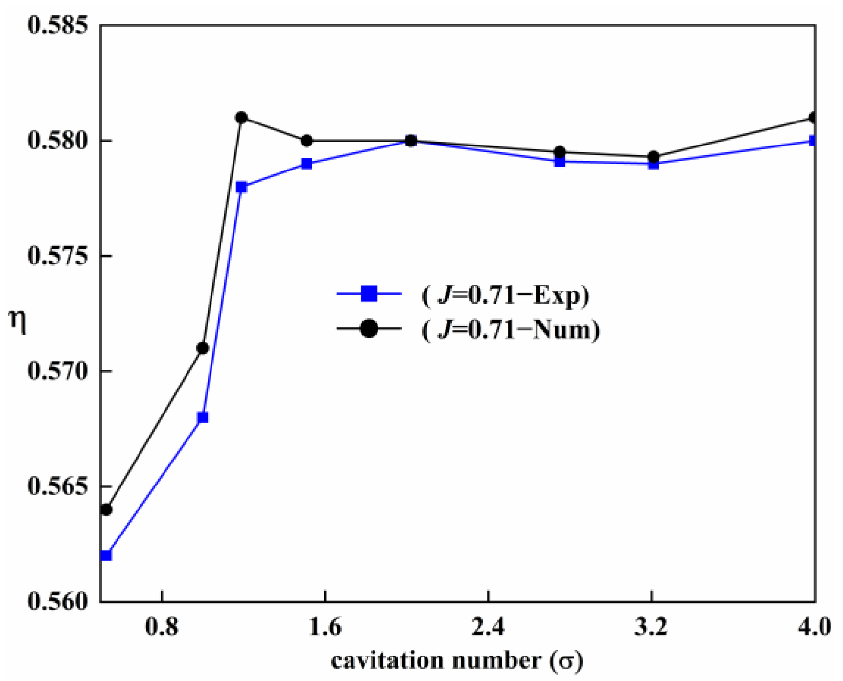
The cavitation model also affects the accuracy of the calculation results. The Z-G-B cavitation model has been used in many studies of PJP or propeller cavitation flow field [16,19,51]. They have verified the validity of the Z-G-B cavitation model by using the E779A propeller with different J values [16,19]. The PJP model used in this study is the same as the PJP model of [16,19]. The Figure 9 shows the difference between CFD values and experimental values at different cavitation numbers. For different cavitation number conditions, the error of propulsion efficiency is relatively small between CFD value and experimental value. All errors are within 2%. The numerical simulation results well agree with the experimental data, which shows that the Z-G-B cavitation model can better simulate the cavitation flow field of PJP.

4.2. Vertification of the Grid Independence

The quality and quantity of grids play a key role in the accuracy of the numerical results. Excess grids will result in the waste of cost and time, while few grids will result in convergence difficulties and low result accuracy. Therefore, grid independence verification is very important for the PJP analysis. The total number of grids can be adjusted by adjusting the first layer grids height and the number of nodes based on previous studies [14,16,19]. According to the theory of [52], the and fine meshes (Fine mesh = 30.26 M, Coarse mesh = 16.62 M) are used to verify the grid influence. The grid-convergence index (GCI) calculated according to the theory of Richardson extrapolation [52] has been used to study the grid-convergence tests. The coarse-grid Richardson error can be calculated using Equations (21)–(23):

$$E_{coarse}=\frac{r^p\epsilon }{1-r^p},$$

(21)

$$\epsilon =f_2-f_1,$$

(22)

$$r={(\frac{N_{fine}}{N_{coarse}})}^{1/d}.$$

(23)

Here, f1 and f2 are the torque and thrust coefficient, respectively, for the two types of meshes [19,53]. P denotes the accuracy of algorithm (p = 2 herein). Additionally, r is the refinement factor for the two meshes, and d is the dimensionality of the CFD simulation. The GCI of the coarse mesh can be determined as follows:

$$GC{I}_{coarse}=F_s\left|E_{coarse}\right|.$$

(24)

$F_s$ > 1 is a safety factor. Herein, $F_s$ = 3.

Rotor thrust and torque coefficient at three different advance ratios (

Table 7. GCI of different grid numbers.

J	Coefficients	Coarse	Fine	Ecoarse	GCIcoarse
1.6075	$K_T$	0.85332	0.85124	0.005659	1.69%
	$K_Q$	0.37943	0.37662	0.007645	2.29%
2.1433	$K_T$	0.70213	0.70012	0.005469	1.64%
	$K_Q$	0.37534	0.37358	0.004788	1.44%
3.2151	$K_T$	0.37694	0.37509	0.005033	1.51%
	$K_Q$	0.32045	0.31935	0.002992	0.89%

) are selected to verify the influence of the number of grids. As shown in Table 7, the GCI of coarse grids is within 3%, and the biggest difference is just 2.29%. This indicates that the number of grids 16.62 M can be used to analysis the PJP under an oblique flow.

5. Results and Discussion

5.1. Hydrodynamic Performance of PJP

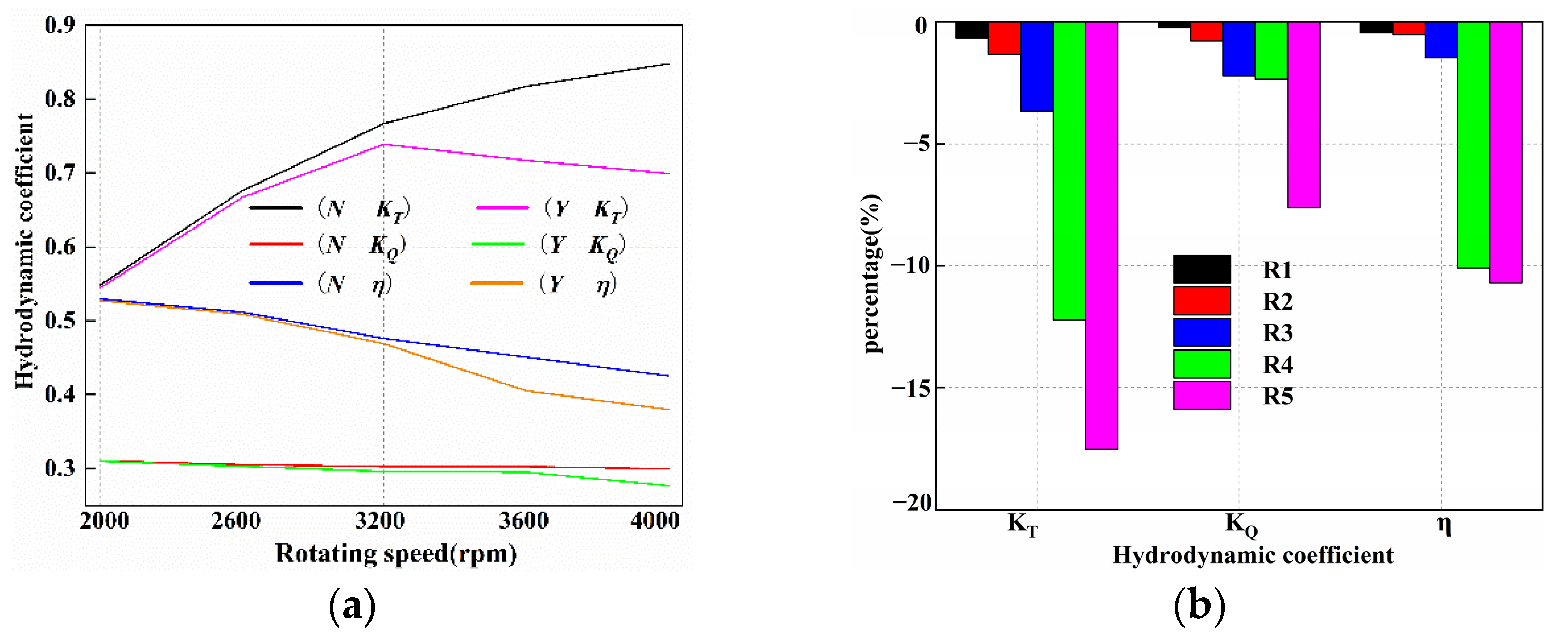
In this section, five rotating speed conditions (R1 = 2000 rpm, R2 = 2600 rpm, R3 = 3200 rpm, R4 = 3600 rpm, and R5 = 4000 rpm) are used to study the cavitation hydrodynamic performance at the oblique flow conditions ($\beta =20°$). As shown in Figure 10a,b, N and Y represent the non-cavitation and cavitation conditions, respectively. In

Table 8. Difference between different rotating speeds.

	N KT (%)	Y KT (%)	N KQ (%)	Y KQ (%)	N η (%)	Y η (%)
${\Delta }_{R2-R1}$	23.31	22.52	−1.76	−2.32	−3.44	−3.52
${\Delta }_{R3-R2}$	13.48	10.81	−0.91	−2.31	−6.96	−7.84
${\Delta }_{R4-R3}$	6.52	−2.93	−0.01	−0.15	−5.31	−13.59
${\Delta }_{R5-R4}$	3.89	−2.49	−1.01	−6.37	−5.64	−6.26

, ${\Delta }_{R2-R1}$ represents the difference in the hydrodynamic parameter between the rotating speeds R2 and R1, and other symbols are similar to ${\Delta }_{R2-R1}$.

The propulsion efficiency $\eta$ in the cavitation and non-cavitation conditions decreased with increasing rotating speeds R1–R5, which is consistent with the results of [16,19]. Table 8 shows that the decrease of the propulsion efficiency is more obvious under higher rotating speed conditions than the lower rotating speed conditions, and the maximum decrease is up to 13.59% when the R = 3200 rpm under cavitation conditions. The change of the rotating speed basically has no effect on the total torque coefficient $K_Q$, exhibiting that the PJP in this study has good balance. For the cavitation condition, the largest drop of total torque coefficient at the high rotating speed of R5 is only 6.37%, while that for the non-cavitation condition is within 2%. At low rotating speeds (such as R1–R3), the total thrust coefficient $K_T$ greatly increases with the rotating speed, where the maximum change range reaches 22.5% (cavitation) and 23.31% (non-cavitation). Furthermore, the change of the total thrust coefficient is relatively small at higher rotating speeds. The above discussion denotes that the PJP efficiency is determined by rotor rotating speed, speed of the incoming flow, thrust coefficient of the rotor and stator, and torque coefficient, etc. Generally, the decline in the propulsion efficiency with the cavitation condition is more obvious than that with the non-cavitation condition. Similarly, Figure 10b shows that the influence of cavitation on the PJP hydrodynamic coefficient becomes more obvious with increasing rotating speeds. Especially, at higher rotating speeds, the efficiency difference between the cavitation and no-cavitation conditions is more obvious, and the maximum difference reaches 12.21%.

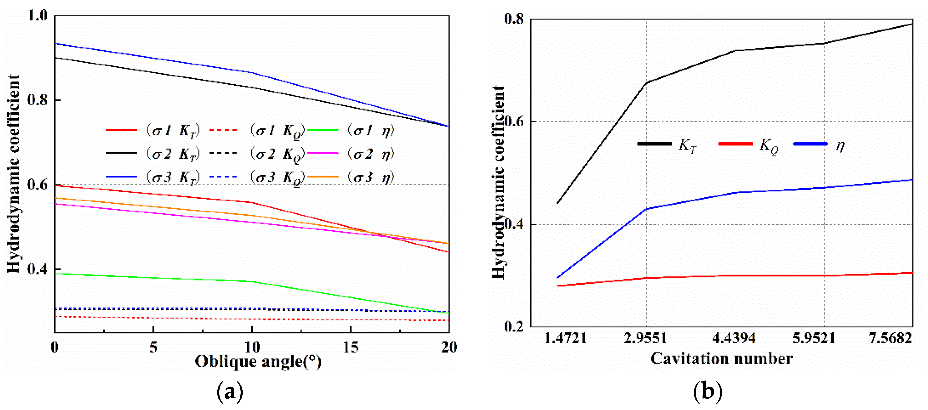
Figure 11a shows the hydrodynamic performance parameters at different oblique angles ($\beta =0°–20°$) and cavitation numbers ($\sigma 1=1.4721,\sigma 2=4.4394,and\sigma 3=7.5682$). In

Table 9. Difference at different cavitation numbers.

	σ1 (%)	σ2 (%)	σ3 (%)
${\Delta }_{0–10}$	−4.65	−7.88	−7.31
${\Delta }_{0–20}$	−24.09	−16.91	−18.93

and

Table 10. Difference at different oblique angles.

	0° (%)	10° (%)	20° (%)
${\Delta }_{\sigma 1–\sigma 2}$	42.56	37.74	56.07
${\Delta }_{\sigma 1–\sigma 3}$	46.13	42.05	56.09
${\Delta }_{\sigma 2–\sigma 3}$	2.49	3.12	1.02

, ${\Delta }_{0–10}$ denotes the difference of hydrodynamic coefficient between $0°$ and $10°$; ${\Delta }_{0–20}$ has a similar meaning. Additionally, ${\Delta }_{\sigma 1–\sigma 2}$ is the difference of hydrodynamic coefficient between $\sigma 1$ and $\sigma 2$; ${\Delta }_{\sigma 1–\sigma 3}$ and ${\Delta }_{\sigma 2–\sigma 3}$ have similar meanings.

Generally, the three hydrodynamic coefficients of PJP decrease with increasing oblique angles. Table 10 shows that a smaller oblique angle, $\beta =10°$, has a relatively small effect on the open water efficiency at three cavitation numbers, with a maximum efficiency loss of only 7.88%. However, the propulsion efficiency significantly changes when $\beta =20°$, with the maximum efficiency loss exceeding 20%. Moreover, the three hydrodynamic coefficients of PJP increase with the cavitation number. For the open water efficiency $\eta$, smaller cavitation numbers $\sigma 1=1.4721$ have a greater impact on efficiency reduction than larger cavitation numbers. As shown in Table 10, the propulsion efficiency decreases by more than 37% regardless of the axial or oblique flow conditions when $\sigma 1=1.4721$. This denotes that the PJP blades have a large cavitation area at $\sigma 1$. However, the difference in the efficiencies between $\sigma 2$ and $\sigma 3$ is relatively small; the biggest difference in efficiency is only 3.12%, which occurs at the oblique angle of $\beta =10°$. Although the cavitation number considerably influences the PJP efficiency, the total torque coefficient remains relatively consistent at different cavitation numbers. Under the three cavitation number conditions, the total torque coefficient only slightly changes with the oblique angle. Figure 11b shows the changing trends of the hydrodynamic coefficient for five different cavitation numbers when $\beta =20°$. The total thrust coefficient $K_T$ and efficiency $\eta$ increase with the cavitation number, and the change range of $K_T$ and $\eta$ is relatively small after $\sigma$ exceeds $\sigma 4=2.9551$. The smaller cavitation number $\sigma 1=1.4721$ has a greater impact on the PJP hydrodynamic performance at oblique flow conditions.

5.2. Analyses the Flow Field Using CFD and Data-Driven Methods

5.2.1. Analysis of the Influence of the Rotating Speed

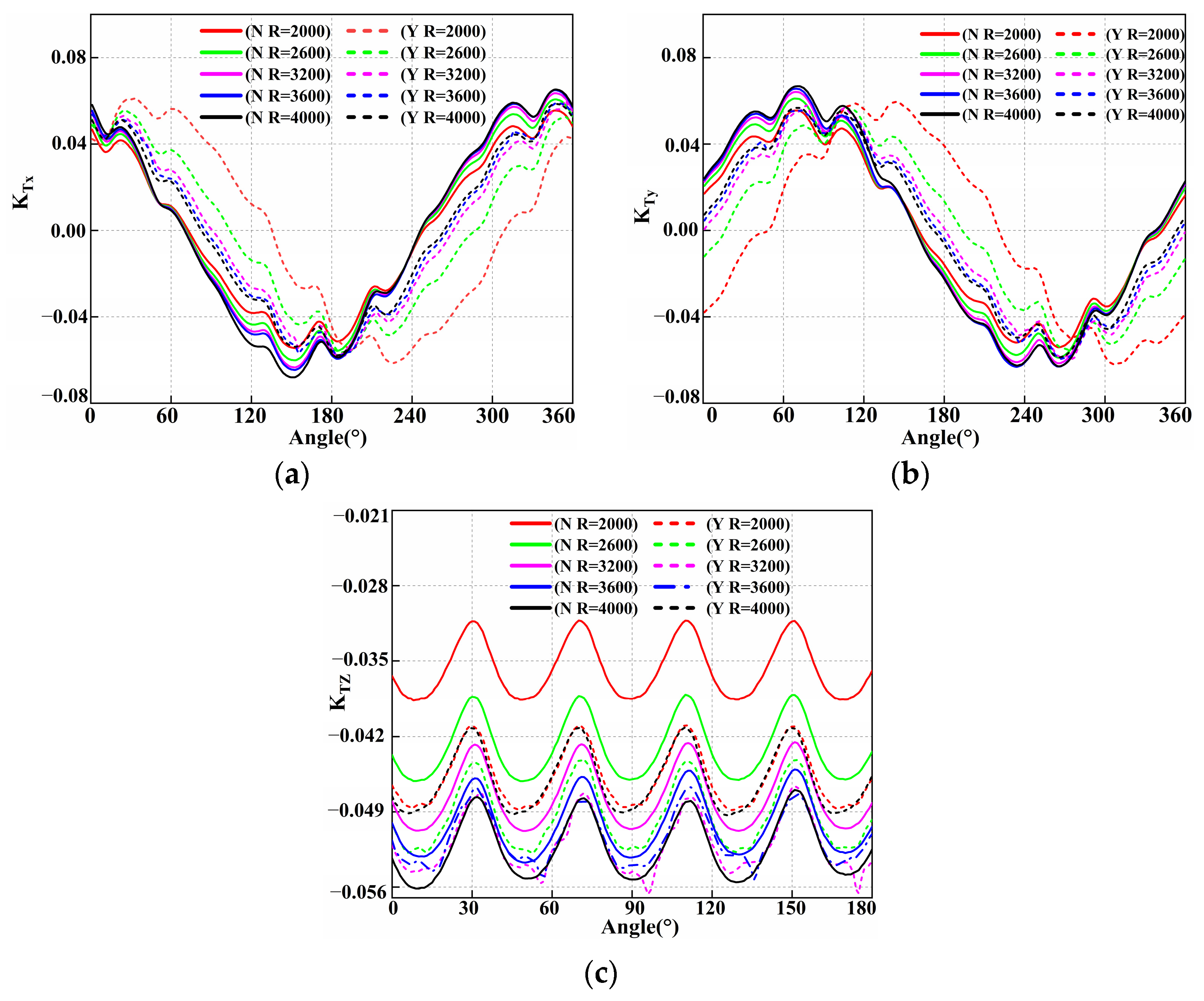
In this section, the cavitation number $\sigma =4.4394$ and oblique angle $\beta =20°$ are used to analyze the influence of the PJP rotating speed. The bearing force comprises the transverse force $K_{TX}$, vertical force $K_{TY}$, and axial force $K_{TZ}$. Figure 12 shows the changing trend of the bearing force with different rotating speeds under the cavitation condition (N) and non-cavitation condition (Y). Under the no-cavitation conditions, Figure 12a shows that for the different rotating speeds, the transverse force $K_{TX}$ only differs in the peak value and there is no phase difference. In contrast, under the cavitation condition, there is not only a difference in the peak values of the transverse force but also a certain phase difference. Moreover, the fluctuation range of the transverse force increases with the rotating speed, and the phase simultaneously shifts to the left. As shown in Figure 12b, the change law of the vertical force $K_{TY}$ with the rotating speed is similar to that of the transverse force. The difference between the transverse and vertical forces is only a certain peak phase difference under the no-cavitation and cavitation conditions. The axial force $K_{TZ}$ still exhibits good periodicity under the two conditions (N and Y) regardless of the rotation speed, which is verified by the pressure cloud in Figure 13. The fluctuation range of the axial force under the cavitation condition is relatively smaller than that under the non-cavitation condition. With increasing rotating speeds, the axial force first increases and then decreases after the rotating speed reaches 3200 rpm. The conclusion is consistent with Figure 10a.

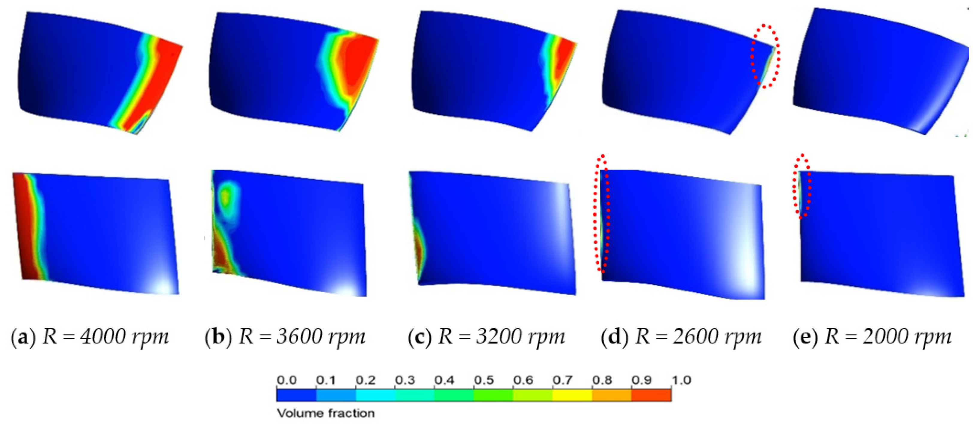
Figure 13 shows the water vapor phase volume fraction cloud of the rotor and stator blades at different rotating speeds. The figure clearly shows that the cavitation area of the rotor and stator blades increases with increasing rotating speeds, and the cavitation phenomenon basically disappears for low rotating speeds R = 2000 and 2600 rpm. For a low rotating speed (such as 3200, 2600, and 2000 rpm), the rotation of the rotor blades affords discontinuities when the fluid passes through the leading edges of the rotor blades. The upper end of the guide edge yields a tip vortex, which causes the local low pressure and cavitation phenomenon (as shown in Figure 13c–e). The fluid flowing through the rotor blades significantly accelerates at high rotating speeds (such as 3600 and 4000 rpm), where the pressure significantly drops, and it can afford a large cavitation area (as shown in Figure 13a,b), especially at the rotor blade tip. Furthermore, the cavitation phenomenon occurs at the suction surface of the stator blades, which occurs due to the influence of the rotor blades. The cavitation area and intensity both increase with increasing rotating speeds, which can further decrease the total thrust of the PJP.

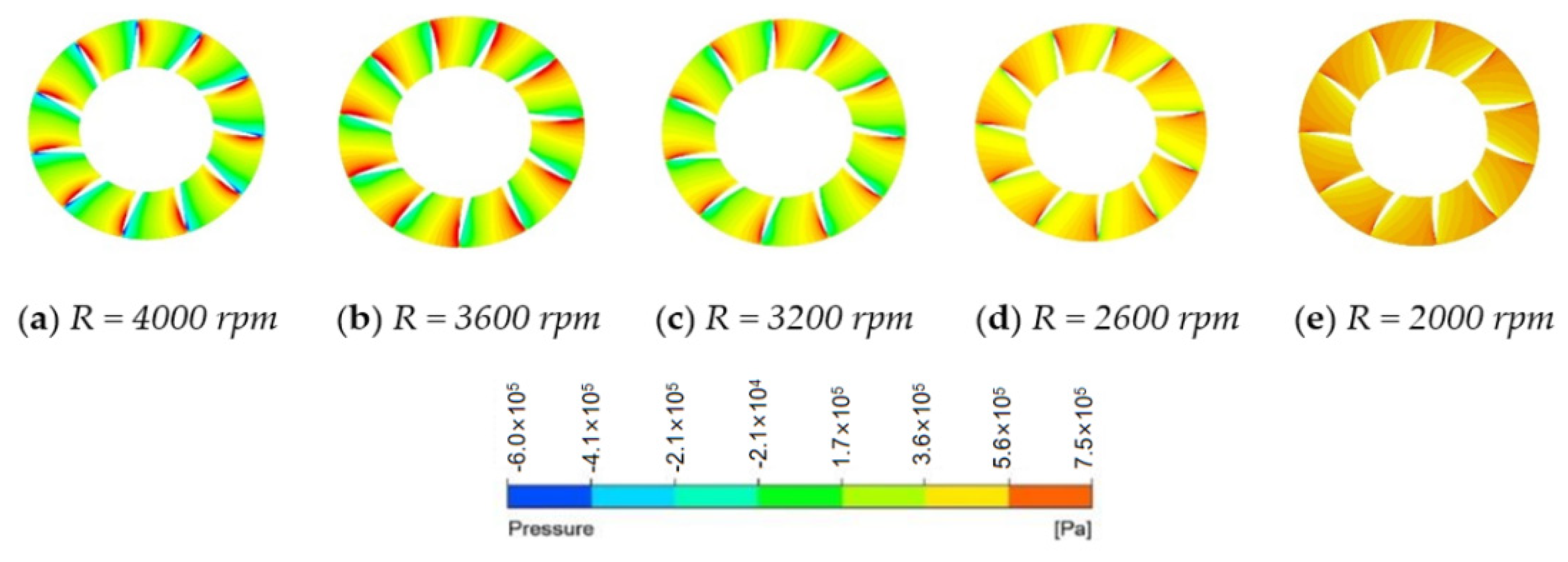
Figure 14 shows the pressure cloud of the rotor domain at different rotating speeds when the oblique angle $\beta =20°$. The pressure distributions on the rotor disc surface at different rotating speeds exhibit obvious differences. The overall pressure of the fluid environment on the rotor disc surface continuously decreases with increasing rotating speed. For any rotating speed, a low-pressure area is present at the suction surface of the rotor disc surface. The low-pressure area continues to expand with increasing rotating speed. The pressure surface of the rotor is not prone to cavitation, which is in a relatively high-pressure area. Moreover, the area of the high-pressure zone decreases with increasing rotating speed. The pressure difference between the pressure and suction surface increases with the rotating speed. This verifies the changing trend of Figure 13: the cavitation area is larger at higher rotating speeds (R = 3600 and 4000 rpm).

The above analysis shows that the transient analysis of the PJP bearing force is an important way to analyze the PJP flow field. A PJP has a complex structure and requires numerous grids; thus, considerable calculation time and resources are required for the numerical simulation of the bearing force using the CFD method until it converges and yields a stable flow field. Thus, a fast and accurate method for predicting the transient bearing forces is extremely important. Herein, the deep neural network model CNN-Bi-LSTM was adopted to obtain the prediction results, which were compared with the CFD results.

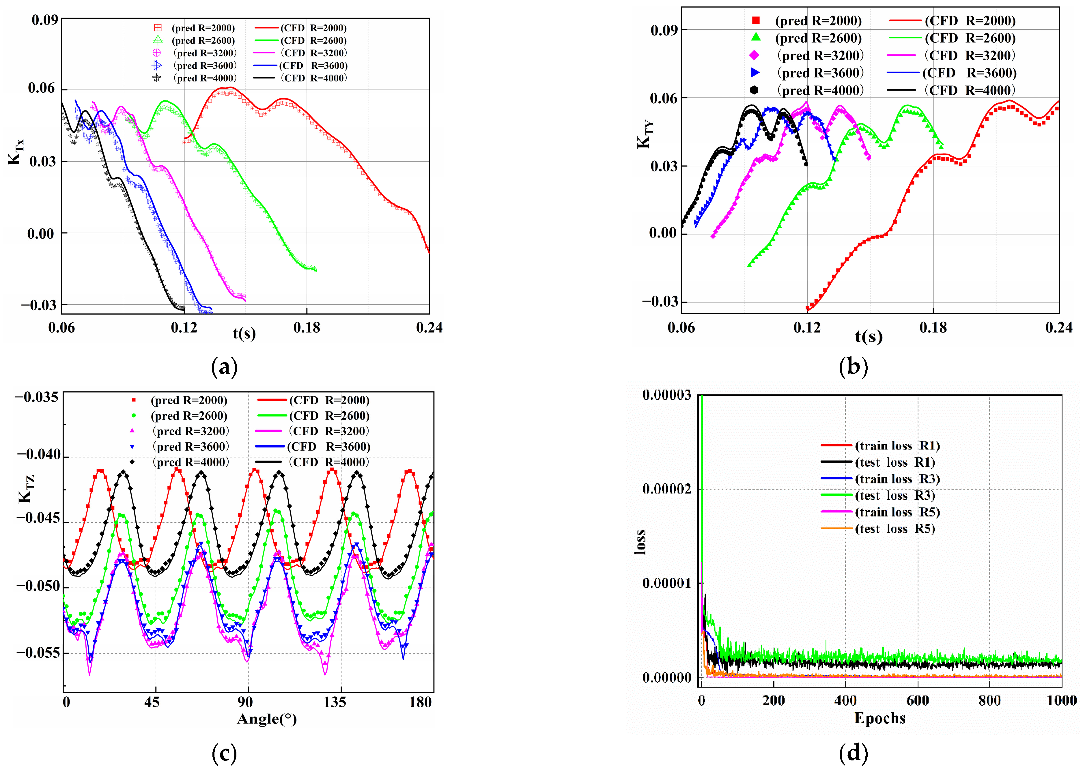
Figure 15 shows the difference in the bearing force between the predicted value (pred) and CFD value at different rotating speeds. Figure 15a clearly shows that the CNN-Bi-LSTM model successfully predicts the phase difference of different rotating speeds and the change trends of the transverse force $K_{TX}$. Other than the position of the transverse force crest value, the predicted values of other positions well agree with the CFD values. This may be due to the relatively large fluctuation of the crest value at five rotating speeds, and the predicted values are within the acceptable error range. For the different rotating speeds, the differences between the predicted peak data and CFD data under lower speed conditions are relatively small compared to those at higher rotating speed conditions (3600 and 4000 rpm), which is because the fluctuations in the same time interval conditions are relatively larger than the crest value of the low rotating speeds. For the vertical force $K_{TY}$, the change trend of the difference between the predicted value and CFD value at different rotating speeds is similar to that for the transverse force. Additionally, the number of cycles of the axial force $K_{TZ}$ is equal to the number of stator blades (Qiu et al., 2020), which has a stronger periodicity than the transverse and vertical forces. Figure 15c shows that the predicted value of the axial force affords a better accuracy than that of the transverse and vertical forces at different rotating speeds. A large error is only present at the trough at the rotating speed R = 3200 rpm. As shown in Figure 15d, the losses of the training and testing datasets converge very quickly and the fluctuation is relatively small, which may be due to the good periodicity of the time series dataset of PJP, and the deep learning method can more easily learn time and the nonlinear relation compared to other methods. The convergence speed and training stability show that the bearing force prediction of PJP requires very little time when using a data-driven method compared to that when using the CFD method. Deep learning methods afford a certain feasibility in the prediction of the PJP bearing force considering the training time and prediction accuracy.

5.2.2. Analysis and Prediction of the Influence of the Oblique Angle and Cavitation Number

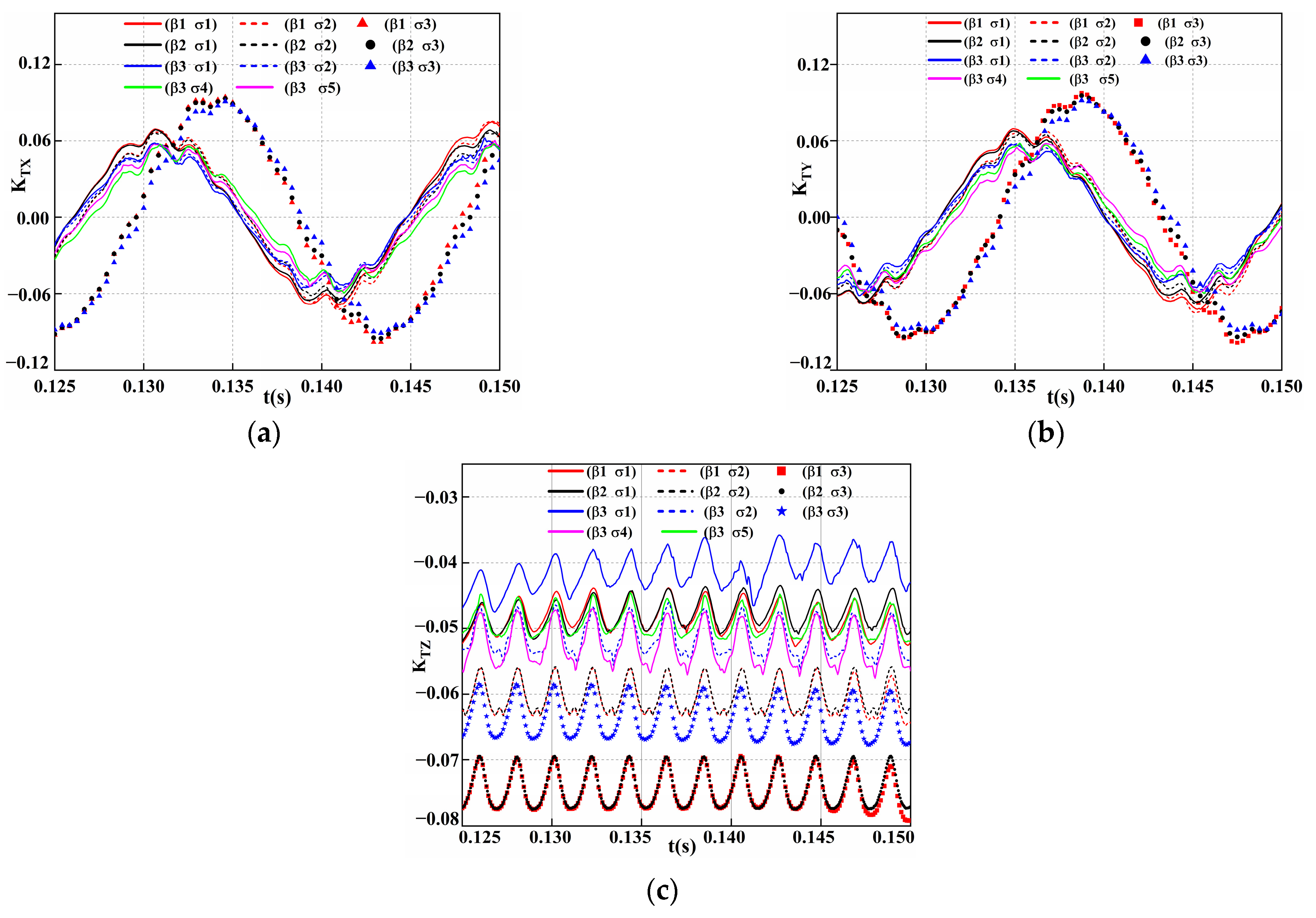
As shown in Figure 16, the cavitation numbers $\sigma 1,\sigma 2,\sigma 3,\sigma 4,\sigma 5$, respectively, are 1.4721, 4.4394, 7.5682, 2.9551, and 5.9225. The oblique flow angles $\beta 1,\beta 2,\beta 3$ are $0°,10°,20°$, respectively. For the same cavitation number, no phase difference exists in the transverse force peak of a single-rotor blade. The peak difference of the transverse force is relatively smaller than that of pure axial flow when $\beta =10°$. While at a higher oblique angle of $\beta =20°$, the peak value of the transverse force is relatively large compared to that of the lower oblique flow angle condition. For different cavitation numbers, the change trends are relatively similar to the pure axial flow condition. The phase and peak difference of the transverse force are relatively small at the lower cavitation numbers $\sigma 1$ and $\sigma 2$. At a higher cavitation number $\sigma 3=7.5682$, the phase difference and peak value of the transverse force significantly change, where the peak value is larger than the smaller cavitation number $\sigma 1$ and $\sigma 2$ conditions. The changing trend of the vertical force $K_{TY}$ is similar to that of the transverse force at different oblique angles and cavitation numbers; only the phase exhibits a certain deviation. For the same oblique angle, the axial force can decrease with increasing cavitation number. The peak value of the axial force reaches the minimum value for the higher cavitation number $\sigma 3=7.5682$. This is similar to the changing trend of the vertical forces: the difference of the peak value is relatively small between $\beta =10°$ and $\beta =0°$, and the peak value of the axial force reaches the maximum when $\beta =20°$.

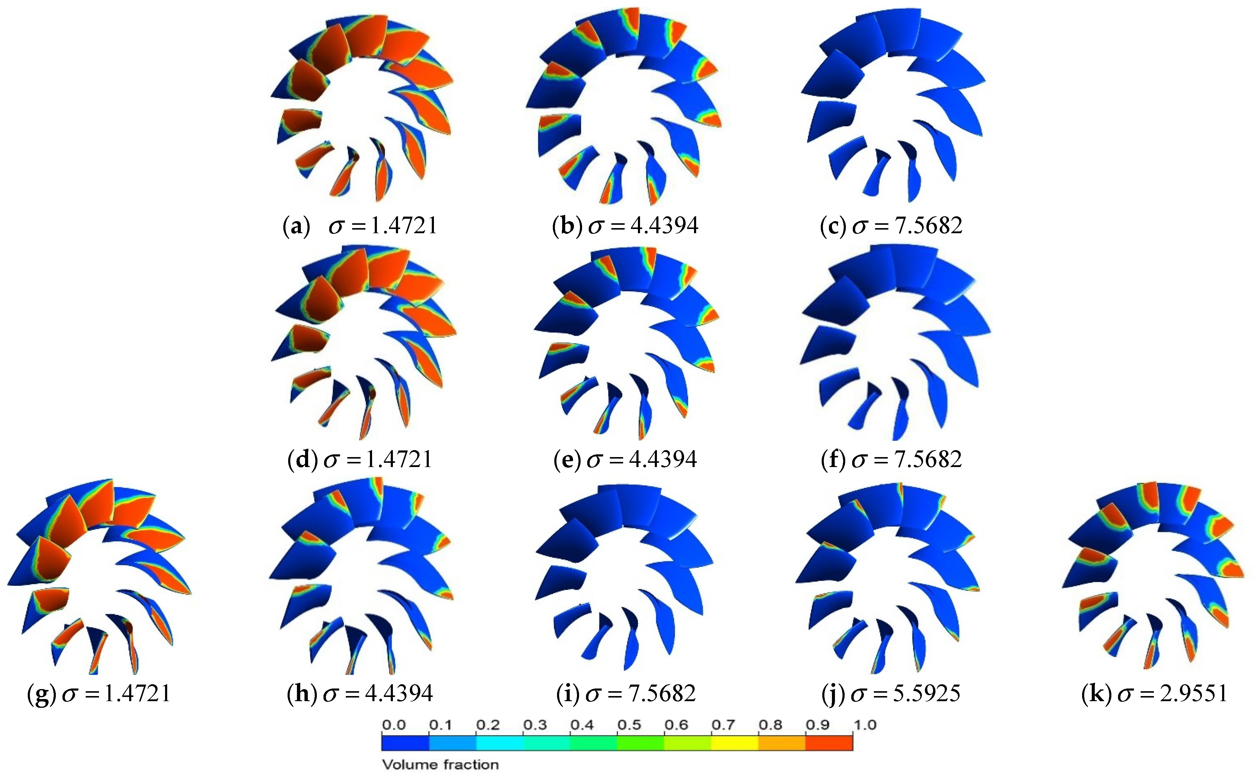
Herein, the rotating speed 3200 rpm is used to study the changing trends of the PJP. Figure 17 shows the tendencies of the water vapor phase volume fraction cloud. For the same $\beta$, the cavitation area of the rotor blade gradually decreases or even disappears with increasing cavitation number, regardless of the oblique flow angle. At the lower cavitation number $\sigma =1.4721$, the cavitation area occupies more than half of the rotor blades area, which is extremely detrimental to the propulsion efficiency of the PJP, which is consistent with the situation mentioned in Section 5.1 where the decline in the propulsion efficiency of PJP is very serious. The difference in the cavitation area is relatively small between $\sigma 3=4.4394$ and $\sigma 3=7.5682$, and the efficiency difference is also small, as shown in Section 5.1.

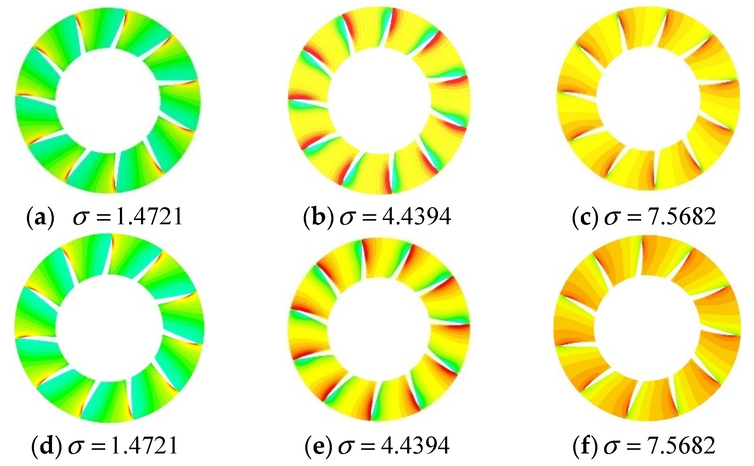
Figure 18 clearly shows that the rotor of the PJP is in a relatively low-pressure area when $\sigma =1.4721$, compared to that with the other two cavitation numbers, which causes the PJP to be more prone to cavitation. As the cavitation number increases, the cavitation phenomenon gradually moves to the rotor blades tip clearance. Figure 18 shows that the pressure of the rotor blades gradually increases with the cavitation number, and the cavitation area of the rotor blades also continuously reduces with increasing pressure difference of the outlet and saturated vapor pressures. The cavitation area difference is relatively small under different oblique flow angles compared to that under different cavitation numbers. Additionally, the water vapor phase volume fraction is higher at the root of the leaf at a higher oblique angle $\beta =20°$, signifying that the rotation of the rotor increases the instability of the PJP flow field under high oblique flow angles. This causes the disc surface of the rotor blades to easily form a low-pressure center, which is conducive to the appearance and development of the cavitation phenomenon. The above phenomenon proves the conclusion that the efficiency (shown in Section 5.1) decreases under higher oblique flow conditions.

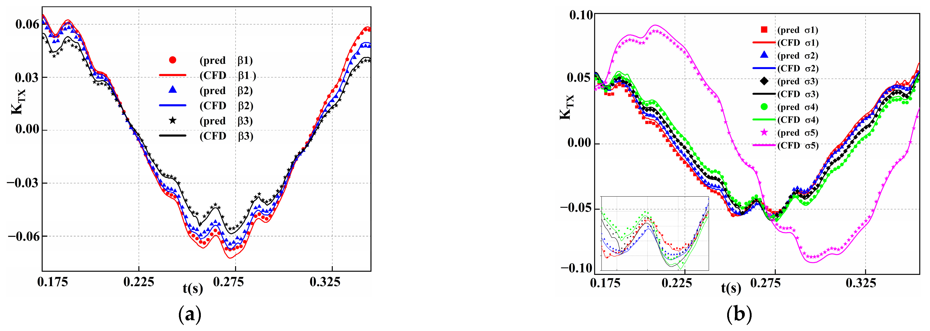
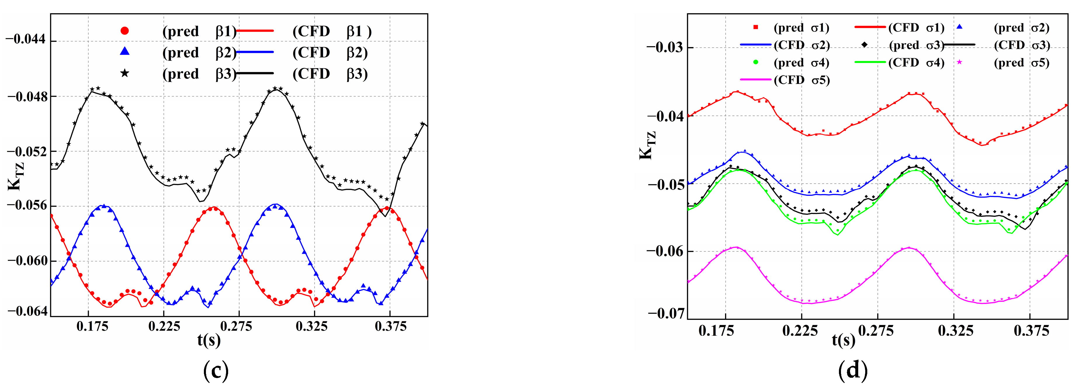
Figure 19 displays the difference between the predicted data and CFD data at different oblique angles and cavitation numbers. The deep neural network model and hyperparameters used here are the same as those in Section 5.2.1. As shown in Figure 19a, CNN-Bi-LSTM not only successfully predicts the trend of transverse force but also affords a better prediction accuracy at the three oblique angles ($\beta 1,\beta 2,\beta 3$). The figure clearly shows that the predicted values of the transverse force, except for that at the trough position, are basically consistent with the CFD values. This is because the fluctuation of this value at the other positions is relatively smaller than that at trough position, and the deep learning model can easily learn the relation between different moments. At the trough position, there is a bigger difference between the predicted and CFD values of the transverse force. The prediction accuracy of the oblique flow condition is higher ($\beta =10°,20°$) than that of the pure axial flow condition ($\beta =0°$). This is because the trough fluctuations under diagonal flow are relatively small. However, the predicted values of the three oblique flow angles are all within the acceptable range. Figure 19b shows the difference between the predicted and CFD values at different cavitation numbers. In Figure 19b, the cavitation number $\sigma 1,\sigma 2,\sigma 3,\sigma 4,\sigma 5$ are 1.4721, 2.9551, 4.4394, 5.9225, and 7.5682, respectively. Overall, the deep model CNN-Bi-LSTM successfully predicts the transverse force at different cavitation numbers. In Figure 19b, the conclusions are similar to those in Figure 19a under the lower cavitation numbers $\sigma 1–\sigma 4$. Under the higher cavitation number $\sigma 5=7.5682$, the fluctuation range and change trend of the axial force exhibit a certain difference compared to those under the smaller cavitation numbers. However, the difference between the predicted and CFD values is relatively large compared to the prediction accuracy with the small cavitation number, which is within the acceptable error range.

Figure 19c,d shows the difference of the axial force $K_{TZ}$ at different cavitation numbers and different oblique angles. The axial force has a good periodicity in a certain time interval and the fluctuation amplitude is relatively small compared to the transverse force. For the lower oblique angles, the predicted value well agrees with the CFD value at the peak and trough positions of the axial force. For the higher oblique angle $\beta =20°$, the axial force at the trough exhibits a relatively large fluctuation compared to that for the lower oblique flow angles, and the difference between the predicted and CFD values is relatively large compared to that for the other two oblique flow working conditions. As shown in Figure 19d, the axial force has similar periodicity at the five different cavitation number conditions, and the predicted values of axial force agree well with the CFD values. Based on the above conclusions, CNN-Bi-LSTM has good generalization ability and can accurately predict the bearing force of a PJP at different oblique flow angles and different cavitation numbers.

5.3. Analysis of the Velocity Field of the Blade Tip Clearances

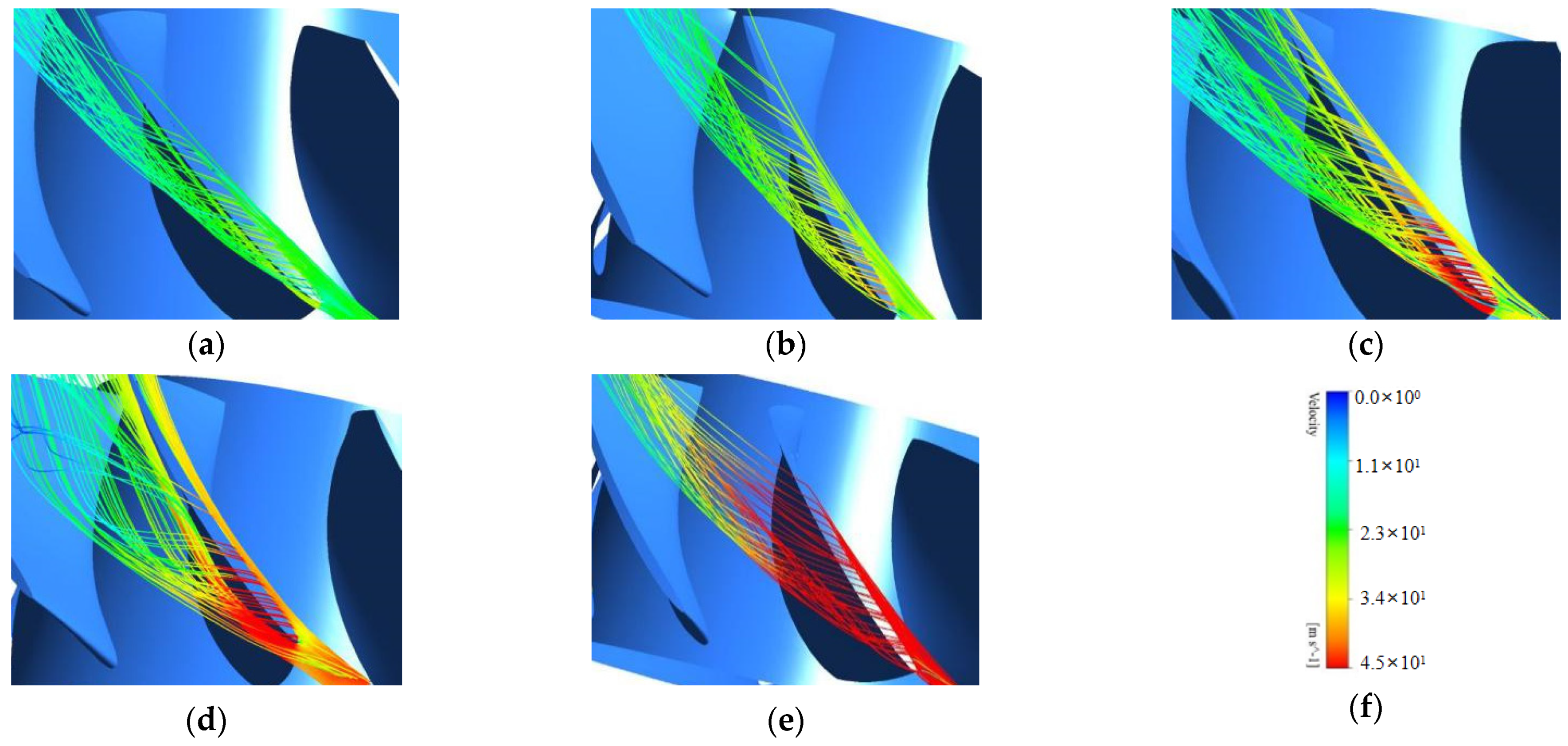
Although the size of the tip clearance is very small, the flow field in the narrow space is the most precise and complex flow field in the entire PJP. The mixing and interaction of the tip clearance flow and the main flow field directly impact the PJP performance. As shown in Figure 20, the velocity streamline of the tip clearance shows that the velocity on the pressure side of the rotor blades is lower than that on the suction side due to the high rotating speed of the rotor blades, which causes the pressure on the pressure side to be higher than that on the suction side. Furthermore, relative movement is present between the high-speed rotation of the rotor and duct, which causes part of the fluid to flow back from the pressure surface to the suction surface and finally form a tip clearance flow in the rotor tip area. The tip clearance flow further develops in the rotor channel to form a local low pressure, which finally forms the tip clearance vortex at the position of the rotor blades tip clearance. Figure 20 shows that the intensity of the tip clearance vortex continuously increases with the rotor rotating speed, and the mixing with the mainstream becomes more intense.

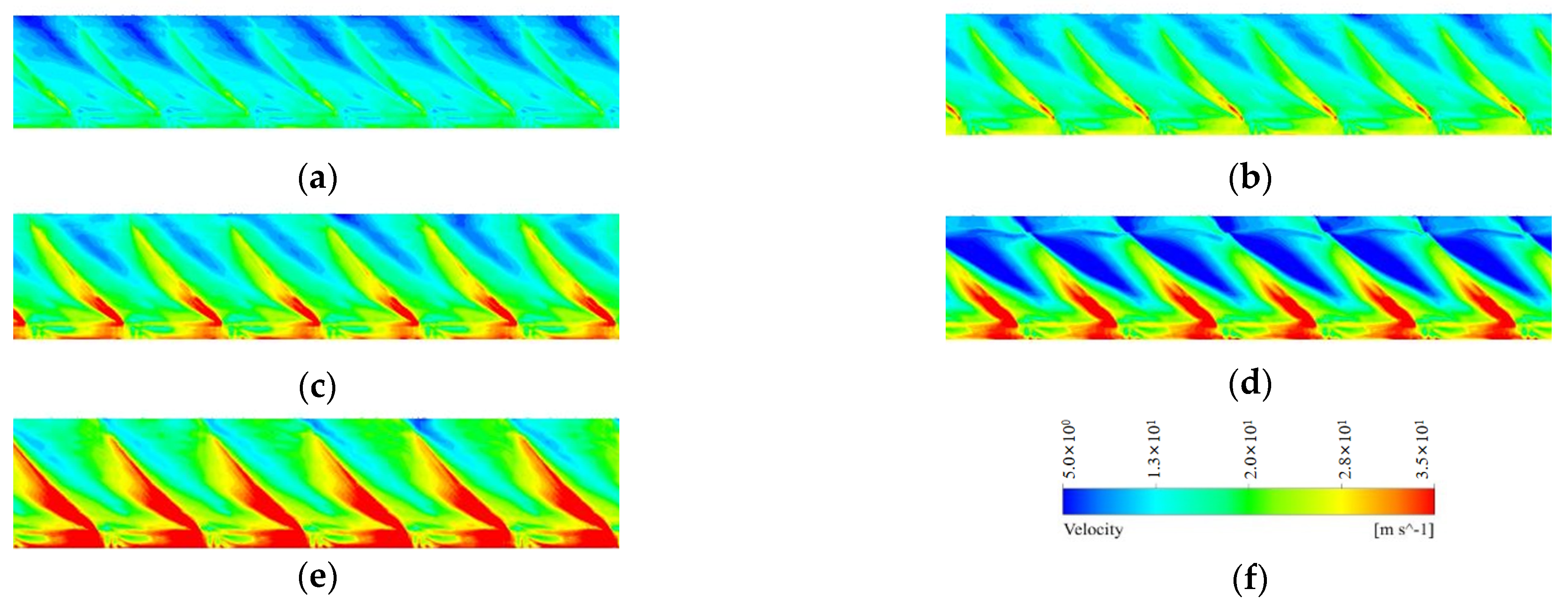
Figure 21 shows the velocity of the rotor blade tip at different rotating speeds when $\beta =20°$. The figure shows that the pressure difference between the pressure and suction sides of the rotor blades gradually increases, and the thrust provided by the rotor blades also increases, proving that the total thrust increases under the high rotating speed condition (R = 4000 rpm). Generally, the velocity is higher near the leading edge of the blade tip, which is mainly caused by the rotation acceleration of the rotor blade, while it is lower on the other side. The area of the low-velocity zone significantly increases with the rotating speed. At higher rotating speeds, the fluid of the rotor domain has higher kinetic energy and higher acceleration of the fluid performance, which provides sufficient space for the tip clearance flow energy to develop and transport. Additionally, the generated tip clearance vortex intensity is higher than that under the lower rotating speed conditions; consequently, more low-velocity areas are afforded at higher rotating speed conditions.

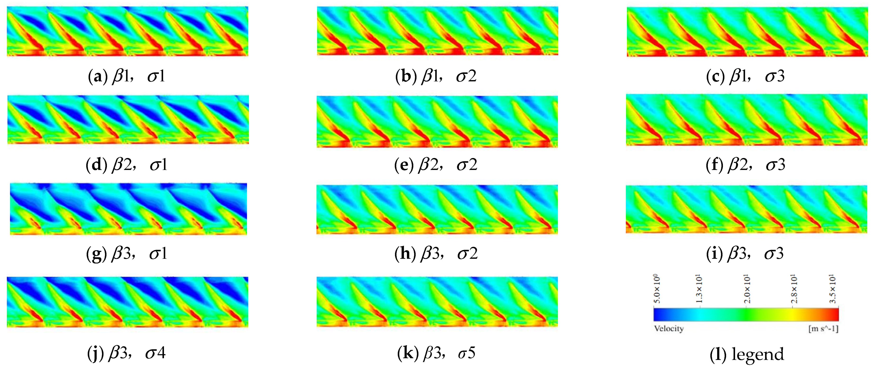
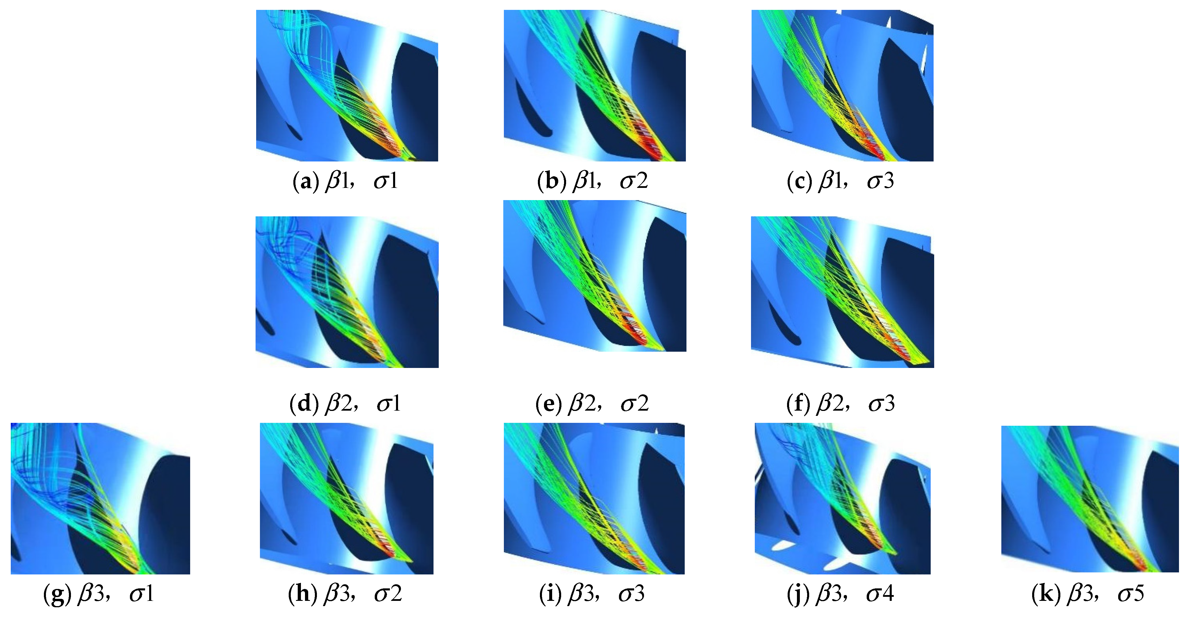
Figure 22 shows the velocity of the rotor blade tip at different oblique angles and cavitation numbers. Clearly, the influence of the cavitation number on the tip clearance flow field is greater than that on the oblique flow angle. Under pure axial flow conditions and $\beta 1=0°$ (Figure 22a–c), the low-velocity area of the rotor suction surface increases with decreasing cavitation number. The sufficient mixing of the low-velocity area and the mainstream affects the rotor domain at the lower cavitation number $\sigma 1=$ 1.4721, which rapidly decreases the open water efficiency. As shown in Figure 22g–k), the situation improves when the cavitation number is increased to $\sigma 2=$ 4.4394, which is consistent with the conclusion of Section 5.1. The change trends under high oblique flow angle ($\beta =10°,20°$) are similar to that under the pure axial flow condition, where the low-velocity regional difference between different cavitation numbers is more obvious under high oblique flow angles condition. For the different oblique angles, as shown in Figure 22a,d,g, the low-velocity area seriously affects the development of the mainstream and the tip clearance vortex core rapidly develops under the high oblique flow angle conditions $\beta 3=20°$. Similarly, Figure 23a,d,g shows that the tip clearance fluid fully develops in the rotor area under a small cavitation number. This proves that high oblique flow angles (such as $\beta 3=20°$) and smaller cavitation numbers (such as $\sigma 1=$ 1.4721 and $\sigma 4=$ 2.9551) are extremely unfavorable for improving the PJP efficiency.

6. Conclusions

Currently, the cavitation phenomenon of PJP has been mainly studied under pure axial flow conditions. This study analyzed the influence of different rotating speeds (R = 2000, 2600, 3200, 3600, and 4000 rpm), different oblique flow angles, and different cavitation numbers (1.4721, 4.4394, 7.5682, 2.9551, and 5.9225) on the hydrodynamic performance, bearing force, and velocity field of PJPs. Moreover, this study proposed a fast and highly accurate deep learning model CNN-Bi-LSTM to solve the problems of traditional numerical simulation methods that consume considerable time and computing resources. Additionally, the SST $k-\omega$ turbulence model and the Z-G-B cavitation model were verified, and found to be in good agreement with the experimental results. The grid independence was verified using three advance ratios. The accuracy of the time sequence datasets of the PJP was verified, and the datasets were reasonably divided. The numerical results revealed that

• The open water propulsion efficiency decreases with increasing rotating speed R. The decrease in the propulsion efficiency is more obvious under high rotating speed conditions, with a maximum decrease of up to 13.59%. The propulsion efficiency significantly changed at the higher oblique angle, with the maximum efficiency loss exceeding 20%. The smaller cavitation numbers 1.4721 significantly impacted the efficiency reduction compared to the other cavitation numbers, with the propulsion efficiency decreasing by more than 37% regardless of the axial flow or oblique flow conditions. Although the cavitation number and rotating speed greatly influence the PJP efficiency, the total torque coefficient remains relatively consistent, signifying that the PJP in this study has good balance.
• The fluctuation ranges of the transverse force $K_{TX}$ and vertical force $K_{TY}$ increase with the rotating speed, which also has a certain difference in phase under different cavitation number conditions. The axial force reaches its maximum value at the rotating speed R = 3200 rpm. The cavitation area and intensity both increase with the rotating speed, which can further reduce the total thrust of the PJP. The cavitation phenomenon basically disappears under low rotating speeds of R = 2600 and 2000 rpm. The peak values of the transverse and vertical forces are relatively large when $\beta =20°$, compared to that under lower oblique flow angles. The axial force always decreases with increasing cavitation number. At the lower cavitation number σ1 = 1.4721, the cavitation area occupies more than half of the rotor blades area, which is extremely detrimental to the PJP propulsion efficiency. The intensity of the tip clearance vortex continuously increases with the rotating speed, which causes the mixing with the mainstream to become more intense.
• The CNN-Bi-LSTM deep learning model successfully predicted the phase difference and change trend of the transverse force $K_{TX}$ and the vertical force $K_{TY}$ under different oblique angles and cavitation numbers. The prediction difference was only large at the crest and trough of the PJP bearing force, which was within the acceptable error range. The predicted value of the axial force exhibited better prediction accuracy than that of the other bearing force due to the better periodicity. The differences between the predicted peak and CFD values under lower speed conditions were relatively small compared to those under larger rotating speed conditions (3600 and 4000 rpm). The prediction accuracy of the oblique flow condition was higher than that of the pure axial flow condition. However, the difference of the larger cavitation numbers was larger than that of the smaller cavitation numbers, which was within the acceptable error range. Using the data-driven method, the convergence speed and training stability require very little time, compared to that using the CFD method.

References

1. Suryanarayana, C.; Satyanarayana, B.; Ramji, K.; Saiju, A. Experimental evaluation of pumpjet propulsor for an axisymmetric body in wind tunnel. Int. J. Nav. Arch. Ocean Eng. 2010, 2, 24–33. [Google Scholar] [CrossRef] [Green Version]
2. Suryanarayana, C.; Satyanarayana, B.; Ramji, K. Performance evaluation of an underwater body and pumpjet by model testing in cavitation tunnel. Int. J. Nav. Arch. Ocean Eng. 2010, 2, 57–67. [Google Scholar] [CrossRef] [Green Version]
3. Amin, T.S.; Mohammad, R.N.; Mojtaba, D.M. Numerical and experimental investigation of the fluid flow on a full-scale pump jet thruster. Ocean Eng. 2019, 182, 527–539. [Google Scholar]
4. Yu, H.; Zhang, G.; Hua, H. Numerical investigation of tip clearance effects on propulsion performance and pressure fluctuation of a pump-jet propulsor. Ocean Eng. 2019, 192, 106500. [Google Scholar] [CrossRef]
5. Yu, H.T.; Duan, N.Y.; Hua, H.X.; Zhang, Z.G. Propulsion performance and unsteady forces of a pump-jet propulsor with different pre-swirl stator parameters. Appl. Ocean. Res. 2020, 100, 102184. [Google Scholar] [CrossRef]
6. McCormick, B.W.; Eisenhuth, J.J. Design and performance of propellers and pumpjets for underwater propulsion. AIAA J. 1963, 1, 2348–2354. [Google Scholar] [CrossRef]
7. Walter, S.G.; Robert, E.H. Selection of a Propulsor for a Submersible System. AIAA J. 1966, 3, 84–90. [Google Scholar]
8. Ivanell, S. Hydrodynamic Simulation of a Torpedo with Pumpjet Propulsion System. Master’s Thesis, Royal Institute of Technology, Stockholm, Sweden, 2001. [Google Scholar]
9. Das, H.N.; Jayakumar, P.; Saji, V.F.; Yerram, R. CFD examination of interaction of flow on high-speed submerged body with pumpjet propulsor. In Proceedings of the 5th International Conference on High Performance Marine Vehicles, Launceston, Australia, 8–10 November 2006; pp. 466–479. [Google Scholar]
10. Dong, Y.; Duan, X.; Feng, S.; Shao, Z. Numerical Simulation of the Overall Flow Field for Underwater Vehicle with Pump Jet Thruster. Procedia Eng. 2012, 31, 769–774. [Google Scholar] [CrossRef] [Green Version]
11. Carreno, J.E.; Mora, J.D.; Perez, F.L. Mathematical model for maneuverability of a riverine support patrol vessel with a pump-jet propulsion system. Ocean Eng. 2013, 63, 96–104. [Google Scholar] [CrossRef]
12. Lv, X.J.; Zhou, Q.D.; Fang, B. Hydrodynamic performance of distributed pump-jet propulsion system for underwater vehicle. J. Hydrodyn. 2014, 26, 523–530. [Google Scholar]
13. Ahn, S.J.; Kwon, O.J. Numerical investigation of a pump-jet with ring rotor using an unstructured mesh technique. J. Mar. Sci. Technol. 2015, 29, 2897–2904. [Google Scholar] [CrossRef]
14. Lu, L.; Pan, G.; Wei, J.; Pan, Y. Numerical simulation of tip clearance impact on a pumpjet propulsor. Int. J. Nav. Arch. Ocean Eng. 2016, 8, 219–227. [Google Scholar] [CrossRef] [Green Version]
15. Lu, L.; Gao, Y.F.; Li, Q.; Du, L. Numerical investigations of tip clearance flow characteristics of a pumpjet propulsor. Int. J. Nav. Arch. Ocean Eng. 2018, 10, 307–317. [Google Scholar] [CrossRef]
16. Pan, G.; Lu, L. Numerical simulation of unsteady cavitating flows of pumpjet propulsor. Ships Offshore Struct. 2016, 11, 64–74. [Google Scholar] [CrossRef]
17. Motallebi-Nejad, M.; Bakhtiari, M.; Ghassemi, H.; Fadavie, M. Numerical analysis of ducted propeller and pumpjet propulsion system using periodic computational domain. J. Mar. Sci. Technol. 2017, 3, 559–573. [Google Scholar] [CrossRef]
18. Wang, C.; Weng, K.; Guo, C.; Gu, L. Prediction of hydrodynamic performance of pump propeller considering the effect of tip vortex. Ocean Eng. 2019, 171, 259–272. [Google Scholar] [CrossRef]
19. Qiu, C.C.; Huang, Q.; Pan, G.; Shi, Y.; Dong, X.G. Numerical simulation of hydrodynamic and cavitation performance of pumpjet propulsor with different tip clearances in oblique flow. Ocean Eng. 2020, 209, 107285. [Google Scholar] [CrossRef]
20. Lu, L.; Wang, C.; Qin, D. Numerical investigations of flow characteristics of a pumpjet propulsor in oblique inflow. Appl. Ocean Res. 2020, 103, 102343. [Google Scholar] [CrossRef]
21. Yuan, J.; Chen, Y.; Wang, L.; Fu, Y.; Zhou, Y.; Xu, J.; Lu, R. Dynamic Analysis of Cavitation Tip Vortex of Pump-Jet Propeller Based on DES. Appl. Sci. 2020, 10, 5998. [Google Scholar] [CrossRef]
22. Liu, C.; Chen, H.X.; Zhang, Z.C.; Ma, Z. Uncertainty analysis of CFD and performance prediction for a pumpjet propulsor. Mod. Phys. Lett. B 2021, 4, 35. [Google Scholar] [CrossRef]
23. Li, H.; Huang, Q.G.; Pan, G. Assessment of transition modeling for the unsteady performance of a pump-jet propulsor in model scale. Appl. Ocean Res. 2021, 108, 102537. [Google Scholar] [CrossRef]
24. Kutz, J.N. Deep learning in fluid dynamics. J. Fluid. Mech. 2017, 814, 1–4. [Google Scholar] [CrossRef] [Green Version]
25. Steven, L.B.; Bernd, R.N.; Petros, K. Machine Learning for Fluid Mechanics. Annu. Rev. Fluid Mech. 2020, 52, 477–508. [Google Scholar]
26. Sekar, V.; Jiang, Q.; Shu, C.; Khoo, B.C. Fast flow field prediction over airfoils using deep learning approach. Phys. Fluids. 2019, 31, 057103. [Google Scholar] [CrossRef]
27. Lee, S.; You, D. Data-driven prediction of unsteady flow over a circular cylinder using deep learning. J. Fluid. Mech. 2019, 879, 217–254. [Google Scholar] [CrossRef] [Green Version]
28. Peng, J.Z.; Chen, S.; Aubry, N.; Chen, Z.H.; Wu, W.T. Time-variant prediction of flow over an airfoil using deep neural network. Phys. Fluids 2020, 32, 123602. [Google Scholar] [CrossRef]
29. Li, B.; Yang, Z.; Zhang, X.; He, G.; Deng, B.Q.; Shen, L. Using machine learning to detect the turbulent region in flow past a circular cylinder. J. Fluid Mech. 2020, 905, A10-1. [Google Scholar] [CrossRef]
30. Wu, H.Z.; Liu, X.J.; An, W. A deep learning approach for efficiently and accurately evaluating the flow field of supercritical airfoils. Comput. Fluids 2020, 198, 104393. [Google Scholar] [CrossRef]
31. Qiu, C.C.; Huang, Q.; Pan, G.; Xing, H. Multi-path deep learning framework on discrete pressure points to predict velocity field of pump-jet propulsor. Appl. Ocean Res. 2022, 123, 103173. [Google Scholar] [CrossRef]
32. Jin, X.W.; Cheng, P.; Chen, W.L.; Li, H. Prediction model of velocity field around circular cylinder over various Reynolds numbers by fusion convolutional neural networks based on pressure on the cylinder. Phys. Fluids 2018, 30, 04705. [Google Scholar] [CrossRef]
33. Wen, S.; Shen, N.W.; Zhang, J.T. Single-rotor UAV flow field simulation using generative adversarial Networks. Comput. Electron. Agric. 2019, 167, 105004. [Google Scholar] [CrossRef]
34. Huang, J.Q.; Liu, H.C.; Ca, W.W. Online in situ prediction of 3-D flame evolution from its history 2-D projections via deep learning. J. Fluid Mech. 2019, 875, 1–12. [Google Scholar] [CrossRef]
35. Miglianti, L.; Cipollini, F.; Oneto, L.; Tani, G.; Gaggero, S.; Coraddu, A.; Viviani, M. Predicting the cavitating marine propeller noise at design stage: A deep learning based approach. Ocean Eng. 2020, 209, 107481. [Google Scholar] [CrossRef]
36. Kong, C.; Chang, J.; Li, Y.; Wang, Z. A deep learning approach for the velocity field prediction in a scramjet isolator. Phys. Fluids 2021, 33, 026103. [Google Scholar] [CrossRef]
37. Deng, Z.; He, C.; Liu, Y.; Kim, K.C. Super-resolution reconstruction of turbulent velocity fields using a generative adversarial network-based artificial intelligence framework. Phys. Fluids 2019, 31, 125111. [Google Scholar]
38. Fukami, K.; Fukagata, K.; Taira, K. Super-resolution reconstruction of turbulent flows with machine learning. J. Fluid Mech. 2019, 870, 106–120. [Google Scholar] [CrossRef] [Green Version]
39. Liu, B.; Tang, J.; Huang, H.; Lu, X.-Y. Deep learning methods for super-resolution reconstruction of turbulent flows. Phys. Fluids 2020, 32, 025105. [Google Scholar] [CrossRef]
40. Kim, H.; Kim, J.; Won, S.; Lee, C. Unsupervised deep learning for super-resolution reconstruction of turbulence. J. Fluid Mech. 2021, 910, A29. [Google Scholar] [CrossRef]
41. Raissi, M.; Yazdani, A.; Karniadakis, G.E. Hidden fluid mechanics: Learning velocity and pressure fields from flow visualizations. Science 2020, 367, 1026–1030. [Google Scholar] [CrossRef]
42. Wang, C.; Sun, S.X.; Sun, S.; Li, L. Numerical analysis of propeller exciting force in oblique flow. J. Mar. Sci. Technol. 2017, 22, 602–619. [Google Scholar] [CrossRef]
43. Ji, B.; Luo, X.; Wu, Y.; Liu, S.; Xu, H.; Oshima, A. Numerical investigation of unsteady cavitating turbulent flow around a full-scale marine propeller. In Proceedings of the 9th International Conference on Hydrodynamics, Shanghai, China, 11–15 October 2010. [Google Scholar]
44. Zhang, D.; Shi, W.; van Esch, B.B.; Shi, L.; Dubuisson, M. Numerical and experimental investigation of tip leakage vortex trajectory and dynamics in an axial flow pump. Comput. Fluids 2015, 112, 61–71. [Google Scholar] [CrossRef]
45. Qin, D.; Pan, G.; Huang, Q. Numerical Investigation of Different Tip Clearances Effect on the Hydrodynamic Performance of Pump-jet Propulsor. Int. J. Comput. Methods 2018, 15, 1850037. [Google Scholar] [CrossRef] [Green Version]
46. Li, H.; Huang, Q.G.; Pan, G.; Dong, X.G. The transient prediction of a pre-swirl stator pump-jet propulsor and a comparative study of hybrid RANS/LES simulations on the wake vortices. Ocean Eng. 2020, 203, 107224. [Google Scholar] [CrossRef]
47. Menter, F.R. Two-equation eddy-viscosity turbulence models for engineering applications. AIAA J. 1994, 32, 1598–1605. [Google Scholar] [CrossRef] [Green Version]
48. Li, F.; Ren, G.R.; Lee, J. Multi-step wind speed prediction based on turbulence intensity and hybrid deep neural networks. Energy Convers. Manag. 2019, 186, 306–322. [Google Scholar] [CrossRef]
49. Wang, Q.; Yang, L.; Rao, Y. Establishment of a generalizable model on a small-scale dataset to predict the surface pressure distribution of gas turbine blades. Energy 2020, 214, 118878. [Google Scholar] [CrossRef]
50. Lecun, Y.; Bottou, L.; Bengio, Y.; Haffner, P. Gradient-based learning applied to document recognition. Proc. IEEE 1998, 86, 2278–2324. [Google Scholar] [CrossRef] [Green Version]
51. Shi, Y.; Pan, G.; Huang, Q.; Du, X. Numerical Simulation of Cavitation Characteristics for Pump-jet Propeller. J. Phys. Conf. Ser. 2015, 640, 012035. [Google Scholar] [CrossRef]
52. Roache, P.J. Quantification of Uncertainty in Computational Fluid Dynamics. Annu. Rev. Fluid Mech. 1997, 29, 123–160. [Google Scholar] [CrossRef] [Green Version]
53. Qin, D.H.; Huang, Q.G.; Pan, G. Comparison of hydrodynamic performance and wake vortices of two typical types of pumpjet propulsor. Ocean Eng. 2021, 224, 108700. [Google Scholar] [CrossRef]
Figure 1. Geometric model of PJP. (a) Pre-swirl rotor; (b) Rotor blades; (c) Stator blades; (d) Pre-swirl stator.
Jmse 10 00918 g001
Figure 2. Computational domain and boundary conditions. The red arrows represent one interpretation of the velocity inlet.
Jmse 10 00918 g002
Figure 3. The difference of two boundary conditions.
Jmse 10 00918 g003
Figure 4. The detailed full structure grid of the PJP.
Jmse 10 00918 g004
Figure 5. Structure of the CNN-Bi-LSTM hybrid model.
Jmse 10 00918 g005
Figure 6. The 1D-CNN structure.
Jmse 10 00918 g006
Figure 7. Bi-LSTM structure.
Jmse 10 00918 g007
Figure 8. Division of the datasets.
Jmse 10 00918 g008
Figure 9. Comparison of CFD values with experimental values at different cavitation numbers.
Jmse 10 00918 g009
Figure 10. Hydrodynamic performance at different rotating speeds. (a) Hydrodynamic parameters at different rotating speeds. (b) Difference among the hydrodynamic parameters.
Jmse 10 00918 g010
Figure 11. Hydrodynamic performance at different oblique angles and cavitation numbers. (a) Hydrodynamic parameters at different oblique angles and cavitation numbers. (b) Difference of the hydrodynamic parameters.
Jmse 10 00918 g011
Figure 12. Bearing force of a single-blade under different conditions. (a) Difference of K T X at different rotating speeds. (b) Difference of K T Y at different rotating speeds. (c) Difference of K T Z at different rotating speeds.
Jmse 10 00918 g012
Figure 13. Water vapor volume fraction cloud of the rotor and stator blades.
Jmse 10 00918 g013
Figure 14. Pressure cloud of the rotor domain at different rotating speeds when β = 20 ° .
Jmse 10 00918 g014
Figure 15. Difference of the bearing force between the predicted value and CFD value. (a) Difference of K T X at different rotating speeds. (b) Difference of K T Y at different rotating speeds. (c) Difference of K T Z at different rotating speeds. (d) Training and testing losses.
Jmse 10 00918 g015
Figure 16. Bearing force of the single-blade at different oblique angles and cavitation numbers. (a) Difference of K T X ; (b) Difference of K T Y ; (c) Difference of K T Z .
Jmse 10 00918 g016
Figure 17. Water vapor phase volume fraction cloud under different oblique angles and cavitation numbers. (Top: β = 0 ° , Center: β = 10 ° , Below: β = 20 ° ).
Jmse 10 00918 g017
Figure 18. Pressure cloud of the rotor domain under different oblique angles and cavitation numbers. (Top: β = 0 ° , Center: β = 10 ° , Below: β = 20 ° ).
Jmse 10 00918 g018aJmse 10 00918 g018b
Figure 19. Difference of K T X and K T Z between the predicted value and CFD value. (a) Difference of K T X at different oblique angles. (b) Difference of K T X at different cavitation numbers. (c) Difference of K T Z at different oblique angles. (d) Difference of K T Z at different cavitation numbers.
Jmse 10 00918 g019aJmse 10 00918 g019b
Figure 20. Velocity streamline diagram of the rotor blade tip at different rotating speeds ((a) 2000rpm; (b) 2600 rpm; (c) 3200rpm; (d) 3600 rpm; (e) 4000 rpm; (f) legend).
Jmse 10 00918 g020
Figure 21. Velocity of the rotor blade tip at different rotating speeds ((a) 2000 rpm; (b)2600 rpm; (c) 3200 rpm; (d) 3600 rpm; (e) 4000 rpm; (f) legend).
Jmse 10 00918 g021
Figure 22. Velocity of the rotor blade tip at different oblique angles and cavitation numbers.
Jmse 10 00918 g022
Figure 23. Velocity streamline of the rotor blade tip at different oblique angles and cavitation numbers.
Jmse 10 00918 g023