A Wet/Dry Point Treatment Method of FVCOM, Part I: Stability Experiments

Abstract

A 3-dimensional wet/dry point treatment method was developed for the unstructured-grid Finite-Volume Community Ocean Model (FVCOM). Analytical equations were derived to examine discretized errors that occurred during the flooding/drying process by the wet/dry point treatment for the flooding/drying process. Numerical experiments were carried out for an idealized estuary, including the inter-tidal zone. The model results show that if the ratio of internal to external mode time steps $(I_{split})$ is appropriately selected, FVCOM was capable of simulating the flooding/drying process with sufficient accuracy to ensure the mass conservation. The up-bound limit of $I_{split}$ was restricted by the bathymetric slope of the inter-tidal zone, external mode time step, horizontal/vertical resolution, and amplitude of tidal forcing at the open boundary, as well as the thickness of the viscous layer specified in the model. Criteria for time steps via these parameters were derived from these experiments, which provide a helpful guide in selecting$I_{split}$ for applying FVCOM to realistic geometric estuaries.

1. Introduction

One of the most challenging problems in estuarine modeling is to provide an accurate simulation of the water transport flooding into and draining out of the intertidal zone. In many estuaries, this transport is comparable to or larger than the transport carried in the main river channel, so its effect on the overall tidal dynamics and salt or nutrient fluxes can be substantial. In the past, two types of approaches have been developed to solve this problem. One is the moving boundary method, and the other is the wet/dry point treatment method. In the first method, the computational domain is bounded by an interface line between land and water, where the total depth and transport normal to the boundary are equal to zero [1]. Because the boundary moves over flooding and drying cycles, the model grid must be re-generated at every time step. This method works for idealized estuaries with simple geometry [2,3], but it is not practical for realistic estuaries with complex geometries, including tidal creeks, islands, barriers, and inlets. In the second method, the computational domain covers the maximum flooding area, with each grid point determined to be either wet or dry as the flow field evolves in time. The wet and dry points are distinguished by the local total water depth $D\left(x,y\right)=H\left(x,y\right)+\zeta \left(x,y,t\right)$ (H is the reference water depth, and $\zeta$ is the surface elevation). A grid point with D > 0 is wet. Otherwise, it is dry. At a dry point, water velocities are automatically set to zero, but the salinity remains the same from the previous time step. Since this method is relatively simple, it has been widely used to simulate the water transport over inter-tidal areas in estuarine models [4,5,6,7,8].

The wet/dry point treatment technique works only in the case where a finite-value solution of the governing equations exists as D approaches zero. In a z-coordinate system, to ensure numerical stability of a 3-dimensional (3D) model, the thickness of the layer closest to the surface must be greater than the amplitude of the tidal elevation [9]. This makes it challenging to apply this method to a shallow estuary in which the amplitude of the tidal elevation is the same order of magnitude as the local water depth. Because irregular bathymetry is difficult to resolve in a z-coordinate model, it is hard to believe that a z-coordinate model can accurately simulate water transport in an intertidal area with realistic, complex bathymetry during both flooding and drying periods [10,11,12,13,14]. In a terrain-following coordinate system, the wet/dry point treatment is no longer valid as D becomes zero. A straightforward way to avoid numerical singularity is to specify zero velocity at all dry points. This approach, however, does not ensure volume conservation in the numerical solution due to discontinuous water removal from elements that turn from wet to dry over one time step. An alternative way is to add a viscous boundary layer (D_min) at the bottom and redefine wet/dry points using a sum of D and D_min. The grid is treated as a wet point for D > D_min. Otherwise, it is a dry point. In terms of the vertical structure of turbulent mixing, a viscous sublayer always exists below the log boundary layer near a solid wall [15]. However, to avoid adding additional water transport into a dynamic system, the viscous sublayer should be sufficiently thin to satisfy a motionless condition. Good examples of the application of this method can be found in [7,8].

No matter which methods are used to simulate the flooding/drying process over the intertidal zone in an estuary, they should be validated with respect to volume conservation. In our previous experiences in implementing a wet/dry point treatment to the semi-implicit Estuarine-Coastal Ocean Model (ECOM-si) [16], a semi-implicit version of the Princeton Ocean Model (POM), we found it is difficult to ensure the salt conservation over the intertidal area [8]. Therefore, checking the volume conservation should be the first step to validating the dry/wet point treatment method. The easiest way is to specify the temperature and salinity constant everywhere as the initial condition and run the model to see if the model can maintain these constant values over the time integration. In any of these methods, the dry and wet points are determined using some empirical criterion so that the computed water transport in the dry-wet transition zone depends on (1) the criterion to define the wet/dry points, (2) the time step used for numerical integration, (3) the horizontal and vertical grid resolutions, (4) the surface elevation amplitude, and (5) the bathymetry. In a terrain-following coordinate system, the transport may also depend on the thickness of the viscous bottom sublayer (D_min). To our knowledge, these issues have not been discussed in detail in previous modeling studies of estuarine intertidal flooding and draining.

This paper describes a wet/dry point treatment method introduced into the unstructured-grid, 3-dimensional (3D) free-surface primitive equation Finite-Volume Community Ocean Model (FVCOM). FVCOM was initially developed by [17] and has been upgraded by the FVCOM development team at the University of Massachusetts and the user community [18,19,20,21,22,23]. We have successfully applied this method to simulate the flooding/drying process in different estuarine systems [24,25,26] and storm- and tsunami-induced coastal inundations [27,28,29,30,31] in the last decades, but the wet/dry treatment methodology implemented in FVCOM was never published. This paper is focused on the stability analysis for an idealized semi-enclosed estuary with an intertidal zone. The relationships of the time step with grid resolution, the amplitude of external forcing, the slope of the inter-tidal area, and the thickness of the viscous bottom layer are discussed, and the criterion for the selection of the time step is derived. The rule used in the model validation is mass conservation, which, we believe, is a prerequisite condition for an objective evaluation of the wet/dry point treatment technique in estuarine models.

2. The FVCOM

FVCOM encompasses seven governing equations: three for momentum, one for incompressible continuity, two for temperature and salinity, and one for density. It is closed mathematically using the Generalized Ocean Turbulent Model (GOTM) for vertical mixing [32] and a Smagorinsky eddy parameterization for horizontal diffusion [33]. The model uses the generalized terrain-following transformation in the vertical to provide a smooth and accurate representation of irregular bottom topography [34].

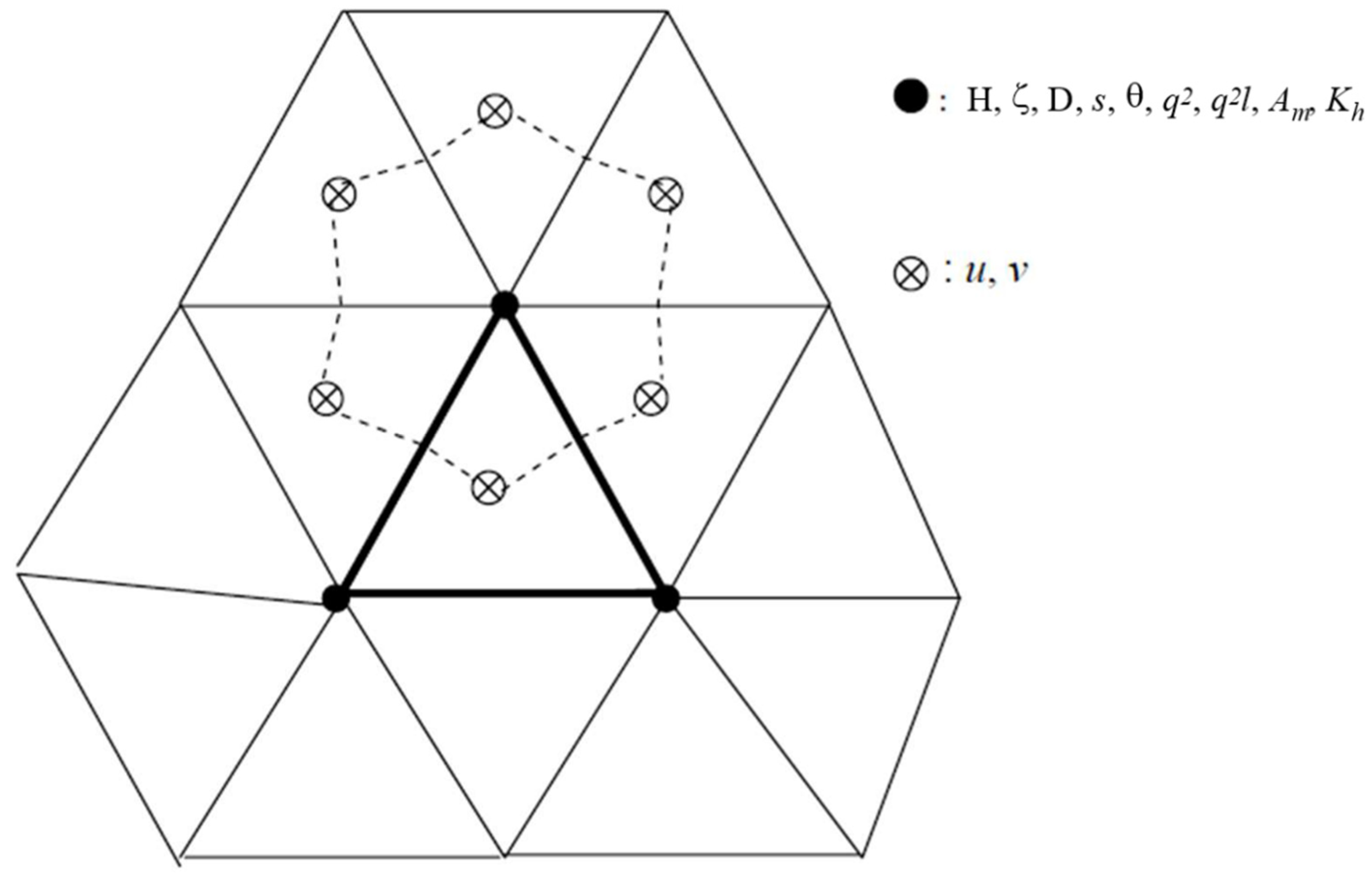
FVCOM subdivides the horizontal numerical computational domain into a set of non-overlapping unstructured triangular cells. Each triangle is comprised of three nodes, a centroid, and three sides (Figure 1), on which the x and y components of the horizontal velocity (u and v) are placed at centroids, and all scalar variables, such as ζ (water elevation), H (reference water depth), D (the total water depth), ω (vertical velocity at the σ-surface), S (salinity), T (temperature), ρ (density), K_m (vertical eddy viscosity), K_h (vertical thermal diffusion coefficient), A_m (horizontal eddy diffusion coefficient), and A_h (horizontal thermal diffusion coefficient) are placed at nodes. Scalar variables at each node are determined by a net flux through the sections linked to centroids and the middle point of the edges in the surrounding triangles (called the tracer control element: TCE), while u and v at centroids are calculated based on the net flux through three sides of that triangle (called the momentum control element: MCE).

FVCOM is solved using the mode-split (external and internal modes) scheme with the updating of the semi-implicit scheme as an alternative choice [21]. The discussion in this paper is aimed at the mode-split method with a σ-coordinate transformation: an open-source version that has been successfully used to simulate the flooding/drying process in various estuaries (http://fvcom.smast.umassd.edu/medm-publications/ (accessed on 30 May 2022)). In this method, the external mode is composed of the vertically integrated transport form of the governing equations. The transport equations are solved for the sea surface elevation $\zeta$ by an explicit difference scheme in which the time step $\Delta t_E$ is constrained by min ($l_1,l_2,l_3)\sqrt{gD},$ where$l_1,l_2,\mathrm{and} l_3$ are the three side lengths of the smallest size triangle, g is gravity, D is the total local water depth, and $\sqrt{gD}$ is the local shallow water wave speed. The internal mode is comprised of the fully 3-dimensional governing equations and solved numerically using a longer time step $\Delta t_I$. The internal mode time step is constrained by the phase speed of the lowest interval wave mode. The linkage between external and internal modes is through $\zeta$. The surface pressure gradients at each $\Delta t_I$ time step in the internal mode are calculated directly by the output of $\zeta$ from the external mode. A second-order accuracy upwind finite-difference scheme is used for flux calculation in the integral form of the advective terms [35,36], and the modified fourth-order Runge–Kutta time-stepping scheme is used for time integration.

In a mode-split model, an adjustment must be made in every internal time step to ensure consistency in the vertically integrated water transport produced by the external and internal modes. In FVCOM, the vertical velocity at the σ-surface (ω) is calculated by

$${\omega }_{i,k+1}={\omega }_{i,k}+\frac{\Delta {\sigma }_k}{\Delta t_I}\left({\zeta }_i^{n+1}-{\zeta }_i^n\right)+\frac{\Delta {\sigma }_k}{{\Omega }_i^n}\underset{l}{\overset{}{{\displaystyle \oint }}}{v}_{N,k}^{n}Ddl$$

(1)

where i, k, and n are the indices of the ith node point, kth σ level and nth time step, respectively, and ${\Omega }_i^n$is the area of the ith TCE at the nth time step. $v_{N,k}^n$indicates the velocity component normal to the boundary of a TCE with a length $l$. To conserve the volume in the ith TCE, the vertically-integrated form of Equation (1) must satisfy

$$\frac{{\zeta }_i^{n+1}-{\zeta }_i^n}{\Delta t_I}+{\displaystyle \sum }_{k=1}^{kb-1}\frac{\Delta {\sigma }_k}{{\Omega }_i^n}\underset{l}{\overset{}{{\displaystyle \oint }}}{v}_{N,k}^{n}Ddl=0$$

(2)

where kb is the total number of the σ-levels. Since ${\zeta }_i^{n+1}$ is calculated through the vertically integrated continuity equation over I_split external mode time steps (where $I_{split}=\frac{\Delta t_I}{\Delta t_E}$), Equation (2) is valid only if

$$\Delta t_I{\displaystyle \sum }_{k=1}^{kb-1}\frac{\Delta {\sigma }_k}{{\Omega }_i^n}\underset{l}{\overset{}{{\displaystyle \oint }}}{v}_{N,k}^{n}Ddl=\Delta t_E{\displaystyle \sum }_{\widehat{n}=1}^{I_{split}}\frac{1}{{\Omega }_i^{\widehat{n}}}\underset{l}{\overset{}{{\displaystyle \oint }}}{\overline{v}}_N^{\widehat{n}}Ddl$$

(3)

Because the numerical accuracy depends on the time step, the left and right sides of (3) are not precisely equal unless I_split = 1. Therefore, to ensure the conservation of the volume transport throughout the water column of the ith TCE, the internal velocity in each σ layer must be calibrated using the difference of inequality of vertically integrated external and internal water transport before ω is calculated. Since the vertically-integrated transport features the barotropic motion, the most straightforward calibration is to adjust the internal velocity by distributing the difference or “error” transport uniformly throughout the water column. ω, which is calculated with adjusted internal velocities through (1), thus guarantees that volume transport is conserved in both the whole water column and the individual TCE volume in each σ layer. Because the water temperature and salinity or other tracers are calculated in the same TCE volume as that used for ω, this transport adjustment also conserves mass in an individual TEC volume in each σ layer.

3. An Unstructured-Grid Wet/Dry Point Treatment Method

The following wet/dry point treatment method has been developed for FVCOM. Similar to our previous practice with ECOM-si [8], we introduce a viscous sublayer with a thickness of D_min into FVCOM to avoid the occurrence of singularity when the local water depth approaches zero. The wet or dry criterion for node points is

$$\left\{\begin{array}{c}\begin{array}{cc}wet,& if D=H+\zeta -h_B>D_{min} \end{array}\\ \begin{array}{cc}dry,& if D=H+\zeta -h_B\le D_{min}\end{array}\end{array}\right.$$

(4)

and for triangular cells is

$$\left\{\begin{array}{c}\begin{array}{cc}wet,& if D=min\left(-h_{B,\widehat{i}},-h_{B,\widehat{j}},-h_{B,\widehat{k}}\right)+max\left({\zeta }_{\widehat{i}},{\zeta }_{\widehat{j}},{\zeta }_{\widehat{k}}\right)>D_{min} \end{array}\\ \begin{array}{cc}dry,& if D=min\left(-h_{B,\widehat{i}},-h_{B,\widehat{j}},-h_{B,\widehat{k}}\right)+max\left({\zeta }_{\widehat{i}},{\zeta }_{\widehat{j}},{\zeta }_{\widehat{k}}\right)\le D_{min}\end{array}\end{array}\right.$$

(5)

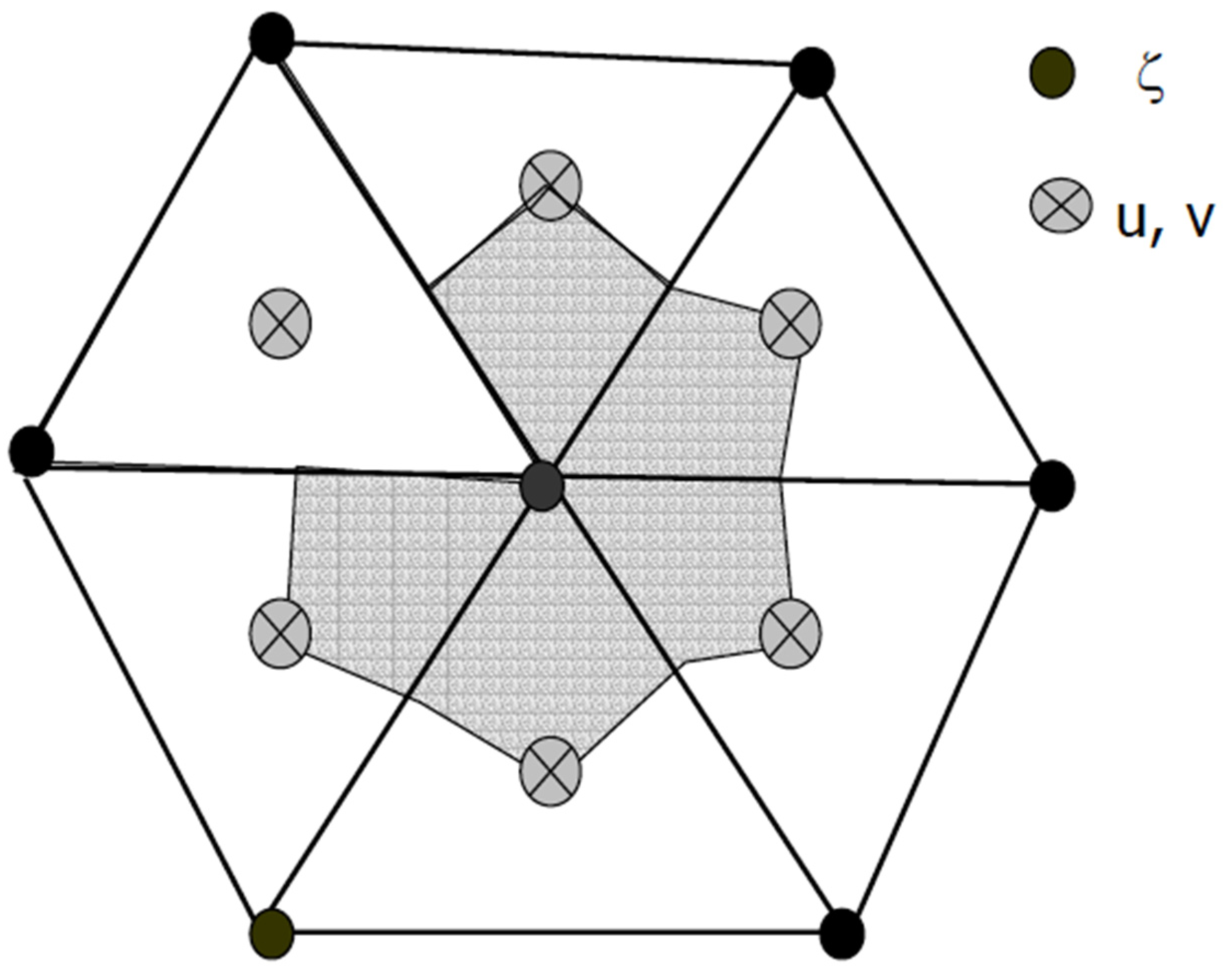
where $h_B$ is the bathymetric height related to the edge of a river where the mean water depth is zero (Figure 2) and $\widehat{i}$, $\widehat{j}$, and $\widehat{k}$ are the integer numbers to identify the three-node points of a triangular cell. When a triangular cell is treated as dry, the velocity at the centroid of this triangle is specified to be zero, and no flux is allowed through the three side boundaries of this triangle. This triangular cell is removed from the flux calculation in the TCE. For example, the integral form of the continuity equation in FVCOM is written as

$${{\displaystyle \iint }}_{TCE}\frac{\partial \zeta }{\partial t}dxdy=-{{\displaystyle \iint }}_{TCE}(\frac{\partial \overline{u}D}{\partial x}+\frac{\partial \overline{v}D}{\partial y})dxdy=-{{\displaystyle \oint }}_l^{}{\overline{v}}_{N}Ddl$$

(6)

where $\overline{ u}$ and $\overline{ v}$ are the x and y components of the vertically-averaged velocity. In a dry/wet point system, only wet triangles are taken into account in the flux calculation in a TCE since the flux on the boundaries of the dry triangle is zero (see Figure 3). This approach always ensures volume conservation in a TCE that contains the moving boundary between the dry and wet triangles. The same procedure is used to calculate the tracer flux (temperature, salinity, and other scalar tracers) and momentum flux in an MCE.

One critical issue in applying the wet/dry point treatment technique in a split-mode model is to ensure mass conservation of individual TCEs which change “state (wet or dry)” one or more times during the I_split external mode integrations made during each internal mode time step; ${\Omega }_i^{\widehat{n}}$ may change within $I_{split}$ external time integrations due to the occurrence of dry triangles and is treated as zero when D is less than $D_{min}$,

$${\zeta }_i^{n+1}-{\zeta }_i^n\ne \Delta t_E{{\displaystyle \sum }}_{n=1}^{I_{split}}\frac{1}{{\Omega }_i^{\widehat{n}}}{{\displaystyle \oint }}_l{\overline{v}}_N^{\widehat{n}}Ddl$$

(7)

In this case, the external and internal mode adjustment through (3) cannot guarantee that ω reaches zero at $\sigma =-1$ for the internal mode. To ensure volume conservation, an additional adjustment for ${\zeta }_i^{n+1}$must be made in the TCE when ω is calculated by (1). The additional sea-level adjustment generally works, but fails in the case where $\zeta$is very close to D_min (for example, $\Delta \zeta =\zeta -D_{min}<{10}^{-1}$(cm)). When this happens, minor errors in calculating the volume flux can rapidly accumulate through nonlinear feedback of tracer advection terms and eventually lead to significant errors in mass conservation.

When $I_{split}$ = 1 (external and internal time steps are identical), FVCOM guarantees mass conservation in the wet-dry transition zone. When computational efficiency requires that $I_{split}$ > 1, several criteria are required to ensure mass conservation in FVCOM. In addition to the criterion for numerical stability, the choice of $I_{split}$ depends on flooding/drying situations: the surface elevation, bathymetry, thickness of the viscous bottom layer, and horizontal/vertical resolutions. A discussion on the relationship of $I_{split}$ with these factors is given next through numerical experiments for several idealized cases.

4. Design of Numerical Experiments

The numerical experiments were conducted for an idealized semi-enclosed channel with a width of 3 km at the bottom, a length of 30 km, a constant depth of 10 m, and a lateral slope of about 0.033 (Figure 4). This channel is oriented east to west, connected to a relatively wide and flat-bottom shelf to the east and intertidal zones along the northern and southern edges. The inter-tidal zone is distributed symmetrically to the channel, with a constant slope of α and a width of 2 km. Our focus was to examine numerical instability due to the nonconservative volume issue resulting from the 2D and 3D mode adjustment in the wet-dry transition zone under the case of $I_{split}\ne 1$. As aforementioned, the finite volume discrete algorithms used in FVCOM ensure volume conservation. However, this conservation law was not valid in the wet-dry transition zone. Choosing a simple idealized geometric problem helped us distinguish the $I_{split}$-related issues from other types of nonlinear instability due to irregular bathymetry changes and complex current interaction over the estuarine-tidal creek-wetland complex. The results obtained from this idealized benchmark testing problem can provide a guide to select $I_{split}$ in real estuarine applications. It was demonstrated in the FVCOM simulation of the Satilla River Estuary, Georgia, US [24].

The computational domain was configured with unstructured triangular grids in the horizontal and σ-levels in the vertical. Numerical experiments were conducted for cases with different horizontal and vertical resolutions. The comparison between these cases was made based on differences from a standard run with a horizontal resolution of about 500 m in the channel, 600 to 1000 m over the shelf, and 600 to 900 m over the inter-tidal zone (Figure 4). In the rest of the text, the standard run refers to the case with the horizontal grid shown in Figure 4 and the following parameters: $\Delta t_E=4.14$ s, I_split = 6, D_min = 5 cm, kb (the number of σ-levels) = 6, and α =7 × 10⁻⁴ (a change of the height of the inter-tidal zone up to 0.8 m over a distance of 2 km in the cross-channel direction). $\Delta t_E$was chosen to satisfy the linear instability criterion constrained by $\min \left(l_1,l_2,l_3\right)/\sqrt{gD}$. In this case, the minimum value of the horizontal resolution over the inter-tidal zone ($\Delta L$) is 600 m.

The model was forced by an M₂ tidal oscillation with amplitude ${\zeta }_o$ at the open boundary over the shelf. This oscillation creates a surface gravity wave that propagates into the channel and reflects after reaching the solid wall at the upstream end. For a given tidal elevation at this open boundary, the velocity in triangular elements connected to the boundary and water transport flowing in and out of the computational domain can be easily determined through the continuity equation.

Specifying an initial distribution of water temperature T = $20$°C and water salinity S = 35 PSU everywhere, we ran the model prognostically with T and S calculated at every internal mode time step. This numerical exercise was done under a pre-condition of numerical stability for the cases with different parameters of $\Delta t_E,$I_split, ${\zeta }_o$, D_min, α, $\Delta L$, and $\Delta \sigma$. In each case, the model was run continuously for 10 model days. According to the law of mass conservation, T and S should remain unchanged over the entire numerical integration for all these cases since there are no external heat and salt sources or sinks in the model problem. Therefore, any change in T and S in the dry-wet transition zone must be due to mass conservation errors during the integration. Since such errors depend primarily on I_split, the upper bound of I_split for given geometric and physical forcing conditions can be defined as the value for which changes in T and S remain small ($\Delta T>$ 10⁻³ °C or $\Delta S>$ 10⁻³ PSU) over the entire (long-term) model integration. Based on this criterion, we can use this idealized case exercise to derive a quantitative relationship of the upper-bound value of I_split with${\zeta }_o$, D_min, α, $\Delta L$, and $\Delta \sigma$.

5. Model Results

5.1. The Standard Case Flooding/Drying Process

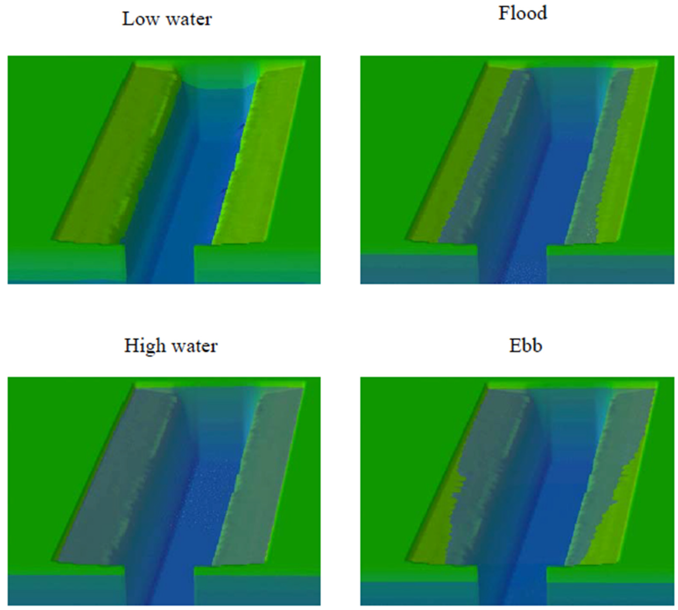
The numerical experiments conducted in this study clearly show that the wet/dry point technique introduced into FVCOM is capable of simulating tide-induced flooding and drying. An example of the model-predicted variation of the water elevation over an M₂ tidal cycle is shown in Figure 5 for the standard case with ${\zeta }_o$ = 1.5 m. During flood tide, the water elevation gradually rises as the inflow of the tidal current increases (Figure 5: the upper-left panel). The water floods onto the intertidal zone when the water level is over the local height (Figure 5: the upper-right panel). The entire inter-tidal zone is covered by water at the transition time from flood to ebb (Figure 5: the lower-left panel0, and then the water drains back into the channel during the ebb tide (Figure 5: the lower-right panel). This flooding/drying process repeats every M₂ tidal cycle, and the model runs stably with $\Delta T$ or $\Delta S$ significantly smaller than 10⁻³ °C or PSU for all time.

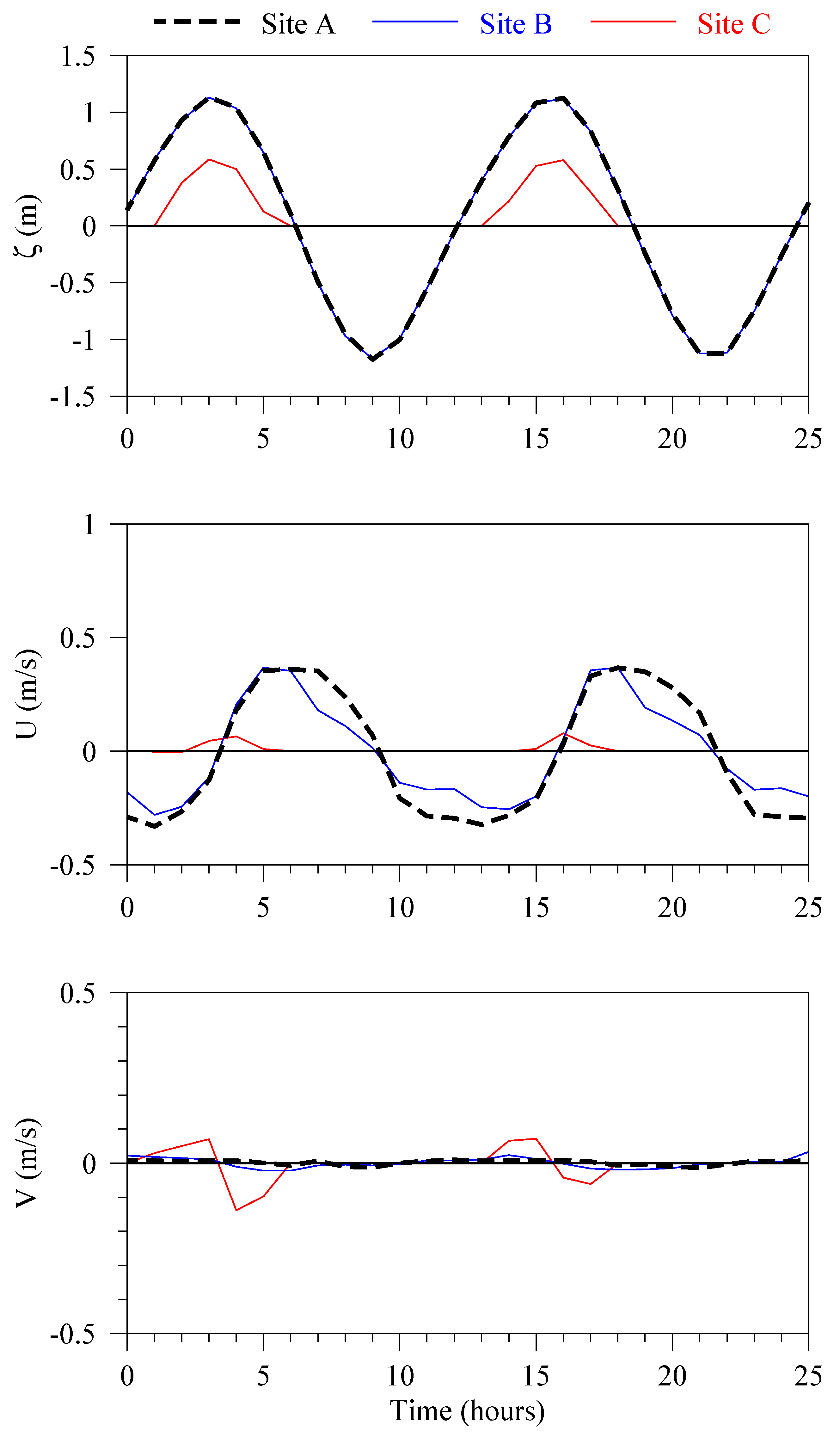
Selecting sites A (at the channel center), B (at the edge of the main channel and intertidal zone), and C (within the intertidal zone), we examined the changes in water elevation ($\zeta$), along-channel current (U), and cross-channel current (V) over tidal cycles (Figure 6). The water elevation at sites A and B were almost identical. They changed stably with an M2 tidal period after a two-tidal cycle spin-up. At site A, the along-channel current was predominant, changing nearly symmetrically over the flood and ebb-tidal periods. At site B, although the water elevation varied symmetrically over the flood and ebb-tidal periods, the currents over the ebb-tidal period varied slowly and lasted much longer. Site C became wet during the flood-tidal period. At that site, the water elevation reached its maximum synchronously with the water change within the channel. The water was drained rapidly during the ebb-tidal period. The change in the cross-channel velocity varied with M₂ tidal cycles due to temporospatial variation of vertical viscosity and horizontal diffusion.

This result suggests that if I_split is appropriately selected, FVCOM can simulate the flooding/drying process with sufficient accuracy that mass conservation errors are insignificant. Clearly, by this criterion, the upper bound for I_split exceeds 6 for the standard case conditions. Next, we consider how the upper bound of I_split depends on the other parameter values.

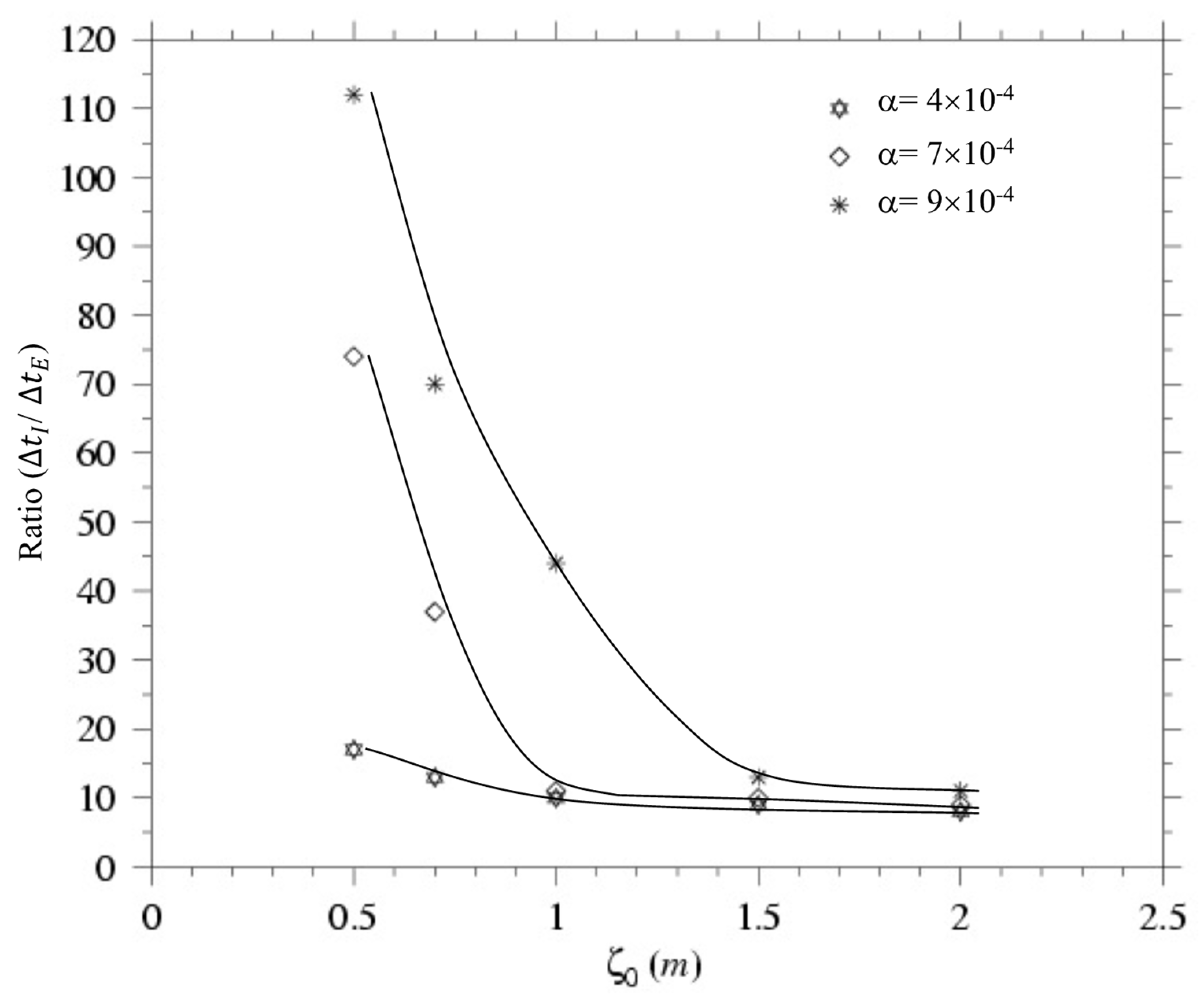
5.2. Relationship with α and ${\zeta }_o$

The upper bound of I_split varies with the slope of the intertidal zone (α) and amplitude of tidal forcing (${\zeta }_o$) (Figure 7). Considering the standard case but with a smaller slope of α = 4.0 $\times {10}^{-4}$, the upper bound of I_split gradually becomes smaller as ${\zeta }_o$ increases. It is below 10 at ${\zeta }_o$ = 2.0 m and up to 15 at ${\zeta }_o$ = 0.5 m. When the slope is increased to 7.0 $\times {10}^{-4}$(a change of the height of the inter-tidal zone bottom up to 1.4 m over a distance of 2 km), however, the upper bound of I_split increases rapidly as ${\zeta }_o$ is decreased below 1.0 m. The model still conserves mass in the wet-dry transition zone at I_split = 70 at ${\zeta }_o$ = 0.5 m. I_split becomes more flexible in the case with the steeper slope of 9.0 $\times {10}^{-4}$ (a change of the height of the inter-tidal zone up to 1.8 m over a distance of 2 km). For all these cases, the upper bound of I_split exceeds 10.

The change in the upper bound of I_split relative to α and ${\zeta }_o$ is consistent with the physics of the flooding/drying process. The flooding speed to cover the intertidal zone during flood increases as α decreases. For a given time step of the external mode, any inconsistency between the external and internal modes becomes more critical to mass conservation as α is decreased, thus the upper bound of I_split must become smaller to conserve mass during the flooding and drying cycle. Since the flooding speed also increases with increasing tidal forcing amplitude ${\zeta }_o$, the inequality shown in Equation (7) becomes more significant for larger ${\zeta }_o$ due to a numerical cutoff of ζ when D < D_min. Thus, the upper bound of I_split generally becomes smaller as ${\zeta }_o$ becomes larger.

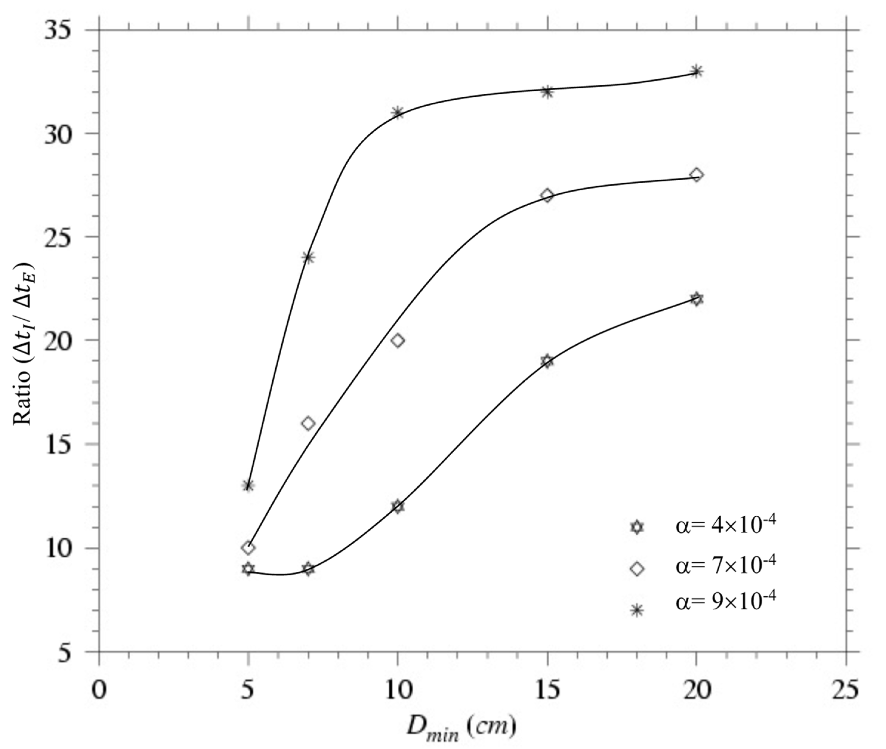
5.3. Relationship with D_min

In general, under given tidal forcing, vertical/horizontal resolution, and external mode time step, the upper bound of I_split increases as the thickness of the viscous layer D_min becomes larger (Figure 8). In the standard case with ${\zeta }_o$ = 1.5 m and α = 4.0 × 10⁻⁴, for example, I_split must be smaller or equal to 9 when D_min = 5 cm but 22 when D_min = 20 cm. I_split could be much larger for a greater bottom slope α of the intertidal zone. In the cases with α = 7.0 × 10⁻⁴ and 9.0 × 10⁻⁴, the upper bound of I_split could be up to 10 and 13, respectively, for D_min = 5 cm and up to 28 and 33, respectively, for D_min = 20 cm.

The relationship of I_split with D_min is not a linear function. The upper bound of I_split tends to converge towards a constant value for D_min > 20 cm in the three cases with different slopes. Increasing D_min directly reduces the occurrence of a negative D in a TCE at the wet-dry edge and thus enhances the numerical consistency between external and internal modes. However, a blind increase of D_min would destroy the physics of flooding/drying by adding too much additional water transport in the wet area, particularly in the shallower inter-tidal zone where the maximum water level might be only 1 to 2 m or less. A value of D_min = 5 cm was found to work well in recent FVCOM simulations of several tidal estuaries in Georgia and South Carolina [24,25], where the maximum flushing area is defined approximately by the 2-m elevation line. The ratio of D_min/max(h_B) equaled 40, sufficiently small to ensure adequate mass conservation in these realistic model applications.

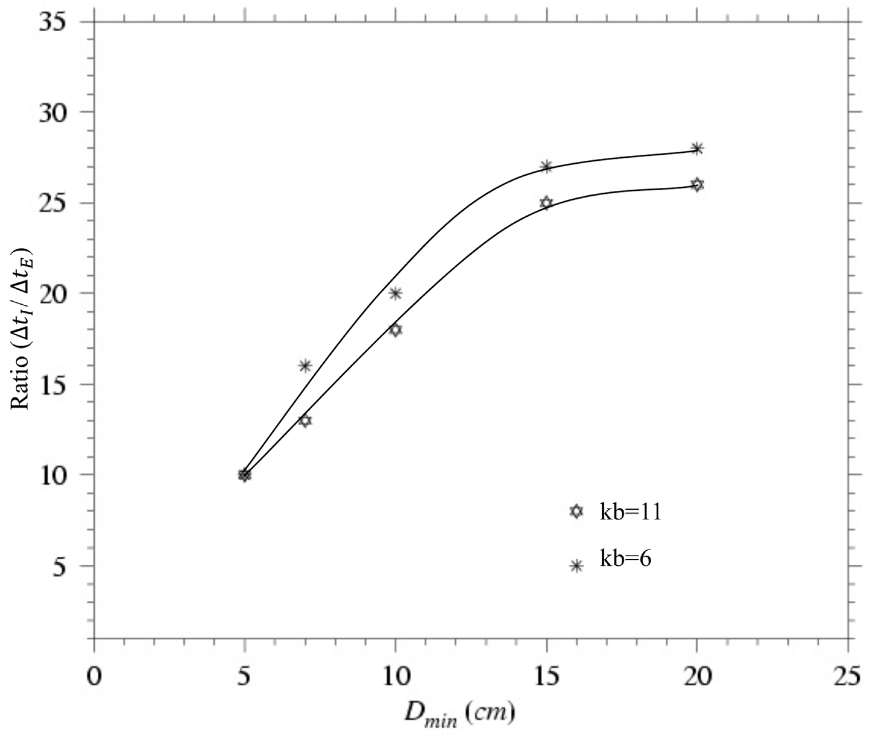
5.4. Relationship with kb

The upper bound of I_split with respect to vertical resolution is sensitive to D_min (Figure 9). For the standard case with kb = 6, α = 7.0 × 10⁻⁴, and ${\zeta }_o$ = 1.5, for example, the upper bound of I_split is 10 for D_min = 5 cm and about 28 for D_min = 20 cm. Keeping the same forcing and geometry but increasing the number of sigma levels kb to 11, the upper bound of I_split remains almost the same for D_min = 5 cm but drops as D_min increases.

In the case with α = 7.0 × 10⁻⁴, defining H = 0 at the edge of the channel, the height of the land at the boundary of the inter-tidal zone is 1.4 m. Considering an amplitude of${\zeta }_o$ = 1.5 m, when the intertidal area is entirely covered by the water during the flood tide, the water elevation at the edge of the intertidal zone should be 10 cm. In the actual numerical computation, however, the water elevation is adjusted by an additional D_min in the region after becoming wet. For a case with D_min = 10 cm, for example, adding D_min is equivalent to double the water elevation at the outer edge boundary of the intertidal zone. In this case, for kb = 6 and 11, the thickness of each σ layer varies from 4 cm and 2 cm (at the outer edge of the intertidal zone) to 32 cm and 16 cm (at the edge of the channel), respectively. When the water is drying in the ebb tide, there are at least 5 layers or 2 layers in a viscous bottom layer of D_min at the wet-dry transition zone for the cases with kb = 11 or 6. Like other coastal ocean models such as POM (Princeton Ocean Model) [37] and ROMs (Regional Ocean Model system) [38], a log-layer dynamics is incorporated into FVCOM, and also this layer could be numerically resolved when the vertical resolution is sufficiently high. Because of the existence of the log layer at the bottom, the model predicts a stronger vertical shear of the current in an additional layer of D_min for kb = 11 than for kb = 6. This shear directly contributes to vertical mixing and destroys the mass conservation in the TCE in the wet-dry transition zone. This is one of the reasons that we found that the up-bound value of I_split reduces as kb increases in a relatively thicker layer of D_min.

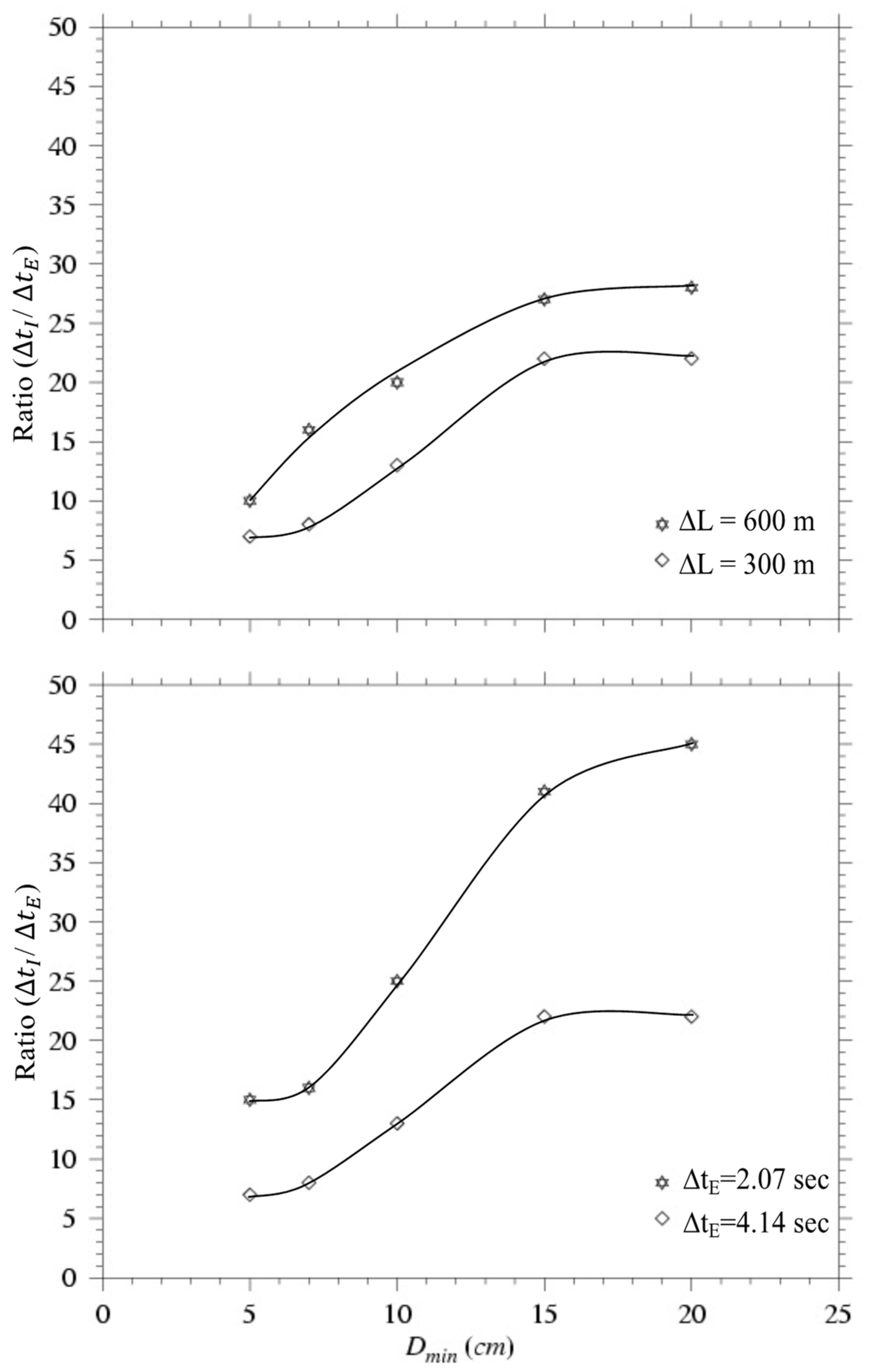
5.5. Relationship with $\Delta L$ and $\Delta t_E$

For a given $\Delta t_E$, the upper bound of I_split decreases as horizontal resolution increases (Figure 10). For the standard cases with${\zeta }_o$ = 1.5 m, for example, the upper bound of I_split is cut off at 10 for D_min = 5 cm and at 28 for D_min = 20 cm. However, these values drop to 7 for D_min = 5 cm and to 21 for D_min = 20 cm when $\Delta L$ is decreased from 600 m to 300 m (Figure 9: upper panel). Similarly, for a given$\Delta L$ = 300 m, the upper bound of I_split increases as $\Delta t_E$ decreases, e.g., I_split jumps from 7 to 15 for D_min = 5 cm and from 21 to 45 for D_min = 20 as $\Delta t_E$ decreases from 4.14 s to 2.07 s (Figure 9: lower panel). In the range of D_min shown in Figure 9, for the two cases with ($\Delta t_E$)₁ and ($\Delta t_E$)₂, (I_split)₂ is approximately estimated by

$${\left(I_{split}\right)}_2~{\left(I_{split}\right)}_1{\frac{{\left(\Delta t_E\right)}_1}{{\left(\Delta t_E\right)}_2}}_{ }.$$

(8)

The fact that the upper bound of I_split drops as $\Delta L$ decreases can be easily understood in view of the geometric change of the tracer control element. For example, when $\Delta L$ is cut in half, a triangle will be divided into 4 triangles. For a given $\Delta t_E$, the possibility for individual triangles to change state (switch from wet to dry or vice versa) is much higher in a high horizontal resolution case than in a low horizontal resolution case. Therefore, I_split should be more restrictive as $\Delta L$ becomes smaller. Similarly, for a given $\Delta L$, the possibility for individual triangles to change state should be less as $\Delta t_E$ becomes smaller, so that I_split should be less restrictive in the case with a smaller $\Delta t_E$.

In addition to satisfying the criterion of numerical stability, how to select $\Delta t_E$ and how to determine $\Delta L$ over the intertidal zone will directly affect the accuracy of the simulated flooding time over the intertidal area. Theoretically speaking, $\Delta L$ and $\Delta t_E$ should be chosen in such a way that the numerical advection velocity (defined as $\Delta L$/$\Delta t_E$) is equal to or smaller than the actual water advection velocity. The failure to satisfy this prerequisite can cause an unrealistic faster flooding speed and exaggerate the horizontal diffusion, thus making the modeled time required for flooding smaller than its actual value.

6. Discussion

The flooding and drying numerical experiments conducted in this study indicate that the upper bound of I_split =$\Delta t_I/\Delta t_E$ depends on factors related to bathymetry, horizontal/vertical resolution, the external mode time step $\Delta t_E$, boundary forcing, and the thickness of the viscous bottom layer. Although the relationship of I_split with these factors is based on simple experiments with an idealized tidal channel with an intertidal zone and a simple criterion of the small net change in conservative water properties like heat and salt, the general patterns drawn from these results should provide a helpful guide for modelers who are interested in applying FVCOM to simulate flooding/drying in estuaries and/or the coastal ocean. We highly recommend that any modeler starting such a study first conduct test experiments (like those described here) with spatially uniform temperature and salinity as a check on their model setup and choice of I_split. If the model temperature and salinity remain constant over time within small limits, then the mass is conserved in the intertidal zone, and FVCOM will produce accurate temperature and salinity fields in experiments with realistic non-uniform, initial temperature and salinity conditions. If the model temperature and salinity change significantly over time from their uniform initial distribution in the test experiment, then the mass is not conserved, and a smaller value of I_split should be considered.

It has been recognized for many years that the Mellor and Yamada [39] level 2.5 turbulence model (called MY-2.5) abruptly shuts down mixing in stratified water when the Richardson number (R_i) rises above 0.25 [40]. When applying MY-2.5 to this idealized estuary (with R_i = 0), we found that it produces a substantial vertical shear of vertical eddy viscosity (K_m) and thermal diffusion coefficient (K_h) in the wet-dry transition zone. Without the inclusion of wind forcing, the model-predicted vertical structure of K_m and K_h reduces to a parabolic shape with a maximum value in the water column no matter how shallow the water is. Thus, the vertical gradient of K_m and K_h can be very large in the wet-dry transition zone, where the value of D-D_min could be just an order of a few centimeters. When this happens, the implicit calculation of the vertical diffusion terms in either momentum or tracer equations can lead to unrealistic velocity or tracer concentration. The unrealistic current speed produced by the MY-2.5 turbulence closure model could be higher than a few meters per second in local wet-dry transition cells. As a result, it can cause the model to blow up numerically within a few time steps.

To avoid this problem, we adjust K_m and K_h in the wet-dry transition region. A simple way is to use the vertically-averaged values of the model-predicted K_m and K_h in the wet-dry transition region. This approach works well in the idealized case discussed in this study and an application to natural estuaries in Georgia and South Carolina. In these and many other realistic applications (e.g., [26]), the height of the inter-tidal zone with respect to the height of the river edge is less than 2 m. A more straightforward alternative approach is to use the vertically-averaged values of the model-predicted K_m and K_h everywhere in the inter-tidal area where it is flushed. Test results show that this approach also works well to avoid the occurrence of unrealistic values of velocity and tracer concentration.

From a physical point of view, the parabolic shape of K_m and K_h is incorrect in a shallow region with vigorous mixing where the vertical depth is an order of a few centimeters. This parabolic distribution is produced by a zero value condition of $q^{2}l$ (where $q^2$ is the turbulent kinetic energy and $l$ is the turbulent macroscale) at the surface and bottom. Clearly, this boundary condition is not valid in a very shallow water region. This raises the dynamic question of whether MY 2.5 or other turbulence closure models should be applied to a shallow estuary with an extensive intertidal zone. This issue must be addressed in future estuarine model development.

7. Summary

A 3-dimensional wet/dry point treatment method has been developed for the unstructured grid finite-volume coastal ocean model FVCOM and tested according to the prerequisite of volume conservation. The model equations were used to examine the reasons for numerical errors produced by mass and volume inconsistencies between the external and internal modes during the simulation of the flooding/drying process. These ideas were tested using numerical experiments for an idealized estuary with an intertidal zone.

The model results indicate that in order to ensure volume and mass conservation during flooding/draining cycles, the ratio of internal to external mode time steps (I_split) is constrained by the amplitude of water elevation, bottom slope, and horizontal/vertical resolution as well as the thickness of the viscous bottom layer specified in the model. The upper bound of I_split increases with an increase in the bottom slope of the intertidal zone (α) or a decrease in the amplitude of tidal forcing (${\zeta }_o$). For a given $\Delta t_E$, the upper bound of I_split decreases as horizontal resolution ($\Delta L$) increases. Similarly, for a given $\Delta L$, the upper bound of I_split increases as $\Delta t_E$ decreases. Although the upper bound of I_split becomes more flexible as the thickness of the viscous bottom layer (D_min) increases, larger values of D_min can lead to an unrealistic simulation of the water transport in the intertidal area and make I_split sensitive to vertical resolution.

These numerical experiments indicate that MY 2.5 leads to unrealistic velocity shears during the flooding/drying process over the intertidal area, particularly in the wet-dry transition zone where the total water depth can be just a few centimeters. Two simple approaches have been introduced to avoid this problem in the inter-tidal area. The question of a more appropriate turbulent mixing scheme to simulate the flooding/drying process in a shallow estuary or coastal area with an extensive flooding area needs further investigation.

References

- Lynch, D.R.; Gray, W.G. Finite element simulation of flow in deforming regions. J. Comput. Phys. 1980, 36, 135–153. [Google Scholar] [CrossRef]
- Sidén, G.L.D.; Lynch, D.R. Wave equation hydrodynamics on deforming elements. Int. J. Numer. Meth. Fluids 1988, 8, 1071–1093. [Google Scholar] [CrossRef]
- Austria, P.M.; Aldama, A.A. Adaptive mesh scheme for free surface flows with moving boundaries. In Computational Methods in Surface Hydrology; Gambolati, G., Rinaldo, A., Brebbiam, C.A., Fray, W.G., Pinder, G.F., Eds.; Springer: New York, NY, USA, 1990; pp. 456–460. [Google Scholar]
- Leendertse, J.J. A Water-Quality Simulation Model for Well-Mixed Estuaries and Coastal Seas: Principles of Computation; Rand Corporation Report RM-6230-RC; RAND Corp.: Santa Monica, CA, USA, 1970; Volume I. [Google Scholar]
- Leendertse, J.J. Aspects of SIMSYS2D, a System for Two-Dimensional Flow Computation; Rand Corporation Report R-3572-USGS; RAND Corp.: Santa Monica, CA, USA, 1987. [Google Scholar]
- Flather, R.A.; Heaps, N.S. Tidal computations for Morecambe Bay. Geophys. J. R. Astron. Soc. 1975, 42, 489–517. [Google Scholar] [CrossRef] [Green Version]
- Ip, J.T.C.; Lynch, D.R.; Friedrichs, C.T. Simulation of estuarine flooding and dewatering with application to Great Bay, New Hampshire. Estuar. Coast. Shelf Sci. 1998, 47, 119–141. [Google Scholar] [CrossRef]
- Zheng, L.; Chen, C.; Liu, H. A modeling study of the Satilla River Estuary, Georgia. Part I: Flooding/drying process and water exchange over the salt marsh-estuary-shelf complex. Estuaries 2003, 26, 651–669. [Google Scholar] [CrossRef]
- Davies, A.M.; Jones, J.E.; Xing, J. Review of recent developments in tidal hydrodynamic modeling, I: Spectral models. J. Hydraul. Eng. ASCE 1997, 123, 278–292. [Google Scholar] [CrossRef]
- Casulli, V.; Cheng, R.T. A semi-implicit finite-difference model for three-dimensional tidal circulation. In Proceedings of the 2nd International Conference on Estuarine and Coastal Modeling, ASCE, Tampa, FL, USA, 13–15 November 1991; pp. 620–631. [Google Scholar]
- Casulli, V.; Cheng, R.T. Semi-implicit finite-difference methods for three-dimensional shallow-water flow. Int. J. Numer. Methods Fluids 1992, 15, 629–648. [Google Scholar] [CrossRef]
- Cheng, R.T.; Casulli, V.; Gartner, J.W. Tidal, residual, intertidal mudflat (TRIM) model and its applications to San Francisco Bay, California. Estuar. Coast. Shelf Sci. 1993, 36, 235–280. [Google Scholar] [CrossRef]
- Casulli, V.; Cattani, E. Stability, accuracy and efficiency of a semi-implicit method for three-dimensional shallow water flow. Comput. Math. Appl. 1994, 27, 99–112. [Google Scholar] [CrossRef] [Green Version]
- Hervouet, J.M.; Janin, J.M. Finite-element algorithms for modeling flood propagation. In Modeling of Flood Propagation over Initially Dry Areas; Molinaro, P., Natale, L., Eds.; ASCE: New York, NY, USA, 1994; pp. 102–113. [Google Scholar]
- Wilcox, D.C. Turbulence Modeling for CFD; DCW Industries, Inc.: La Canada, CA, USA, 2000; 540p. [Google Scholar]
- Blumberg, A.F. A Primer for ECOM-si; Technical Report; HydroQual, Inc.: Mahwah, NJ, USA, 1992; 66p. [Google Scholar]
- Chen, C.; Liu, H.; Beardsley, R.C. An unstructured, finite-volume, three-dimensional, primitive equation ocean model: Application to coastal ocean and estuaries. J. Atmos. Ocean. Technol. 2003, 20, 159–186. [Google Scholar] [CrossRef]
- Chen, C.; Beardsley, R.C.; Cowles, G. An unstructured grid, finite-volume coastal ocean model (FVCOM) system, Special Issue entitled “Advances in Computational Oceanography”. Oceanography 2006, 19, 78–89. [Google Scholar] [CrossRef] [Green Version]
- Chen, C.; Cowles, G.; Beardsley, R.C. An Unstructured-Grid, Finite-Volume Coastal Ocean Model: FVCOM User Manual, 2nd ed.; SMAST/UMASSD Technical Report-06-0602; University of Massachusetts-Dartmouth: New Bedford, MA, USA, 2006; p. 315. [Google Scholar]
- Chen, C.; Huang, H.; Beardsley, R.C.; Liu, H.; Xu, Q.; Cowles, G. A finite-volume numerical approach for coastal ocean circulation studies: Comparisons with finite difference models. J. Geophys. Res. 2007, 112, C03018. [Google Scholar] [CrossRef]
- Chen, C.; Beardsley, R.C.; Cowles, G.; Qi, J.; Lai, Z.; Gao, G.; Stuebe, D.; Liu, H.; Xu, Q.; Xue, P.; et al. An Unstructured-Grid, Finite-Volume Community Ocean Model FVCOM User Manual, 4th ed.; SMAST/UMASSD Technical Report-13-0701; University of Massachusetts-Dartmouth: New Bedford, MA, USA, 2013; p. 404. [Google Scholar]
- Cowles, G.W. Parallelization of the FVCOM coastal ocean model. Int. J. High Perform. Comput. Appl. 2008, 22, 177–193. [Google Scholar] [CrossRef]
- Huang, H.; Chen, C.; Cowles, G.W.; Winant, C.D.; Beardsley, R.C.; Hedstrom, K.S.; Haidvogel, D.B. FVCOM validation experiments: Comparisons with ROMS for three idealized barotropic test problems. J. Geophys. Res.-Ocean. 2008, 113, C07042. [Google Scholar] [CrossRef] [Green Version]
- Chen, C.; Qi, J.; Li, C.; Beardsley, R.C.; Lin, H.; Walker, R.; Gates, K. Complexity of the flooding/drying process in an estuarine tidal-creek salt-marsh system: An application of FVCOM. J. Geophys. Res. 2008, 113, C07052. [Google Scholar] [CrossRef] [Green Version]
- Huang, H.; Chen, C.; Blanton, J.O.; Andreade, F.A. Numerical study of tidal asymmetry in the Okatee Creek, South Carolina. Estuar. Coast. Shelf Sci. 2008, 78, 190–202. [Google Scholar] [CrossRef]
- Zhao, L.; Chen, C.; Vallino, J.; Hopkinson, C.; Beardsley, R.C.; Lin, H.; Lerczak, J. Wetland-estuarine-shelf interaction in the Plum Island Sound and Merrimack River in the Massachusetts Coast. J. Geophys. Res.-Ocean. 2010, 115, 1–13. [Google Scholar] [CrossRef] [Green Version]
- Beardsley, R.C.; Chen, C.; Xu, Q. Coastal flooding in Scituate (MA): A FVCOM study of the 27 December 2010 nor’easter. J. Geophys. Res.-Ocean. 2013, 118, 6030–6045. [Google Scholar] [CrossRef] [Green Version]
- Chen, C.; Beardsley, R.C.; Luettich, R.A., Jr.; Westerink, J.J.; Wang, H.; Perrie, W.; Xu, Q.; Dohahue, A.S.; Qi, J.; Lin, H.; et al. Extratropical storm inundation testbed: Intermodal comparisons in Scituate, Massachusetts. J. Geophys. Res.-Ocean. 2013, 118, 5054–5073. [Google Scholar] [CrossRef] [Green Version]
- Chen, C.; Lai, Z.; Beardsley, R.C.; Sasaki, J.; Lin, J.; Lin, H.; Ji, R.; Sun, Y. The March 11, 2011 Tōhoku M9.0 Earthquake-induced Tsunami and Coastal Inundation along the Japanese Coast: A Model Assessment. Prog. Oceanogr. 2014, 123, 84–104. [Google Scholar] [CrossRef] [Green Version]
- Chen, C.; Lin, Z.; Beardsley, R.C.; Shyka, T.; Zhang, Y.; Xu, Q.; Qi, J.; Lin, H.; Xu, D. Impacts of sea-level rise on future storm-induced coastal inundations over Massachusetts coast. Nat. Hazard 2021, 106, 375–399. [Google Scholar] [CrossRef]
- Zhang, Z.; Chen, C.; Beardsley, R.C.; Li, S.; Xu, Q.; Song, Z.; Zhang, D.; Hu, D.; Guo, F. A FVCOM study of the potential coastal flooding in Apponagansett Bay and Clarks Cove, Dartmouth Town (MA). Nat. Hazard 2020, 103, 2787–2809. [Google Scholar] [CrossRef]
- Burchard, H. Applied Turbulence Modeling in Marine Waters; Springer: Berlin/Heidelberg; Germany; New York, NY, USA; Barcelona, Spain; Hong Kong, China; London, UK; Milan, Italy; Paris, France; Tokyo, Japan, 2002; 215p. [Google Scholar]
- Smagorinsky, J. General circulation experiments with the primitive equations, I. The basic experiment. Mon. Weather Rev. 1963, 91, 99–164. [Google Scholar] [CrossRef]
- Pieterzak, J.; Jakobson, J.B.; Burchard, H.; Vested, H.J.; Petersen, O. A three-dimensional hydrostatic model for coastal and ocean modeling using a generalized topography following coordinate system. Ocean Model. 2002, 4, 173–205. [Google Scholar] [CrossRef]
- Kobayashi, M.H.; Pereira, J.M.C.; Pereira, J.C.F. A conservative finite-volume second-order-accurate projection method on hybrid unstructured grids. J. Comput. Phys. 1999, 150, 40–45. [Google Scholar] [CrossRef]
- Hubbard, M.E. Multidimensional slope limiters for MUSCL-type finite volume schemes on unstructured grids. J. Comput. Phys. 1999, 155, 54–74. [Google Scholar] [CrossRef]
- Blumberg, A.F.; Mellor, G.L. A description of a three-dimensional coastal ocean circulation model. Three-Dimens. Coast. Models 1987, 4, 1–16. [Google Scholar]
- Haidvogel, D.B.; Beckmann, A. Numerical Ocean Circulation Modeling; Imperial College Press: London, UK; 318p.
- Mellor, G.L.; Yamada, T. Development of a turbulence closure model for geophysical fluid problems. Rev. Geophys. 1982, 20, 851–875. [Google Scholar] [CrossRef] [Green Version]
- Kantha, L.H.; Clayson, C.A. An improved mixed layer model for geophysical applications. J. Geophys. Res. 1994, 99, 25235–25266. [Google Scholar] [CrossRef]
Figure 1.
Locations of velocity and tracer variables in the unstructured grid of FVCOM.
Figure 2.
The definitions of H, and hB in a cross-shelf view of the lateral section of an idealized channel, including the intertidal zone.
Figure 3.
Illustration of dry and wet segments of a tracer control element.
Figure 4.
Unstructured triangular grid for the standard run plus a schematic view of the cross-channel section. The dashed line along the channel indicates the edge of the channel connected to the inter-tidal zone. Labels A, B, and C are the locations where the surface elevation (), along-channel current (U), and cross-channel current (V) are displayed.
Figure 5.
A 3-D view of the flooding/drying process over an M2 tidal cycle.
Figure 6.
Time series of water elevation (). along-channel (U), and cross-channel (V) at sites A, B, and C.
Figure 7.
The model-derived relationship of the ratio of the internal to external mode time steps () with the tidal forcing amplitude () and the bathymetric slope of the intertidal zone (α). In these experiments, = 4.14 s, kb = 6, and Dmin = 5 cm.
Figure 8.
The model-derived relationship of with the thickness of the viscous bottom layer (Dmin) for the three cases with α = 4.0 × 10⁻⁴, 7.0 × 10⁻⁴ and 9.0 × 10⁻⁴. In the three cases, = 4.14 s, kb = 6, and = 1.5 m.
Figure 9.
The model-derived relationship of with Dmin for the two cases with kb = 6 and 8, respectively. In these two cases, = 4.14 s, α = 4.0 × 10⁻⁴, and = 1.5 m.
Figure 10.
The model-derived relationship of with (upper panel) and (lower panel). In the upper panel case, = 4.14 s, α = 7.0 × 10⁻⁴, kb = 6, and = 1.5 m. In the lower panel case, = 300 m, α = 7.0 × 10⁻⁴, kb = 6, and = 1.5 m.